Macroeconomics of Systemic Risk: Transmission Channels and Technical Integration

Abstract

The avenue to find a balanced assessment of systemic financial institutions needs the integration of macro and micro granular datasets. This paper investigates how macroeconomic shocks affect systemic risk through several transmission channels. Employing Indonesia datasets over 2008–2019, we regressed three market models: CoVaR, MES, and SRISK using fixed effect, random effect, GARCH(1,1), and finite mixture models. The findings show that stock beta, market index, and exchange rate volatility amplify the systemic risk while the liquidity spread outcome varies due to different of model variables and the deepness of the country’s financial market. We propose a practical systemic risk assessment framework and samples of technical integration to capture the overall risk endogenously and externally expose the systemically important financial institutions.

1. Introduction

Systemic risk methodologies nowadays mainly focus on individual Systemically Important Financial Institutions (SIFIs) and investigate their failure to impact the financial system using publicly available data. The European Central Bank advised the importance of two side interaction between the bank as the individual financial institution to the economy (ECB 2009). De Bandt and Hartmann (2000), in their paper on systemic risk survey, showed that few researchers considered the analysis of macroeconomic indicators that might be behind contagious default. Bisias et al. (2012), under a different survey, listed that the macroeconomic indicators used in systemic risk analytics are now starting to develop after the 2008 financial crisis. Sample studies of various blocks of systemic risk variables stem from macroeconomics like exchange rate (Mayordomo et al. 2014; Yesin 2013) and GDP growth (Festić et al. 2011; Hirtle et al. 2016; Schleer and Semmler 2015). However, despite rising efforts using macroeconomic indicators to study systemic risk, it is estimated separately using the stress test scenarios. The absence of an integrated study of macro-micro assessment of systemic risk raises questions: (1) how macroeconomics affects systemic risk, (2) what variables could bring externality to the SIFIs, and (3) how to integrate the macro and micro granular data into a unified framework and technical calculation of systemic risk? A comprehensive understanding of economic impacts to address the financial contagion issue will provide regulators and policymakers with a holistic approach.

This study aims empirically to investigate how the macro variables propagate SIFIs impacts via specific transmission channels. In addition, the study also provides some technical calculation samples to integrate the macroeconomic variables into their systemic risk assessment. The paper fills the gap by combining the Basel indicator-based model and macroeconomic variables to assess the Systemically Important Banks (SIBs) from two-side (micro and macro perspective). The results would be useful for the policy-makers and bank supervisor in their efforts to determine the SIFIs and their impact on the financial system-wide.

The manuscript employs three robust empiric approaches to systemic risk quantification: CoVaR (Adrian and Brunnermeier 2016), Marginal Expected Shortfall—MES (Acharya et al. 2012), and SRISK (Brownlees and Engle 2017). The models are regressed using fixed effect, random effect generalized least square (GLS), random effect maximum likelihood estimator (MLE), GARCH(1,1), and finite mixture models (FMM) utilize Indonesia banking datasets over 2008–2019. Further, this manuscript also proposes a practical update of the assessment framework together with technical integration calculation to better capture the overall risk. Outcomes of research will contribute to the systemic risk study and improve the overall quantification risk of the financial system.

The findings are as follows: (1) stock beta, market index volatility, and exchange rate volatility does amplify the transmission of systemic risk. In addition, the change in anchor interest rate by policymakers is also significantly proven by statistics though the effect varies among the market models. The difference could come from the employed methods variables and the impact is also different for each interest rate time horizon. Furthermore, related to the liquidity spread, the outcome is a mixture of models. (2) proposes some practical improvement steps in the systemic risk assessment framework to better capture the potential macroeconomic shocks. This study also suggests samples of technical integration calculation and ratios reflecting on the added steps. The integrated macro and micro granular data could portray the overall risk endogenously and externally expose the systemically important financial institutions.

As the discussion progresses, the paper is structured as follows: Section 2 discusses the literature review, containing previous papers and highlighting the possible channel of macroeconomic shocks connected to the systemic risk study. Section 3 contains data details and the methodology framework used. Section 4 presents the analytical results and interpretation, and Section 5 accommodates the conclusion and policy recommendations.

2. Literature Review

2.1. Macroeconomics and Financial Crises

Studies on systemically important banks and systemic risk often incorporate a mixture of variables both micro-level, or bank balance sheets, and macroeconomic data. The European Central Bank advised the importance of two side interactions with banks as the individual financial institutions to the economy (ECB 2009). In their paper, De Bandt and Hartmann (2000) highlighted the discrepancies of using the macroeconomic indicators behind contagious default. However, after their survey in 2000, there was an increasing number of systemic risk academics who used macroeconomic indicators to build the financial stress index in some countries and model the systemic risk. Similarly, Bisias et al. (2012), under a different survey, listed the macroeconomic indicators used in systemic risk analytics as asset-price boom, property price, macroprudential regulation, GDP stress test, risk topography, and several others. Some papers investigate the macroeconomics connection to systemic risk such as de Mendonça and Silva (2018) who used $\mathsf{\Delta }$CoVaR to analyse the Brazilian bank over 2011–2015, highlighting the importance of bank liquidity, profitability, leverage, and interest rate to assess systemic risk. The study noticed that leverage increases the systemic risk because banks become more vulnerable to the shocks. Additionally, higher returns and increase of monetary policy rate also amplify the systemic risk. On the other hand, more proportion in liquidity total assets could lower the systemic risk. Tram and Thi Thanh Hoai (2021) elaborated on the connection of macroeconomics and systemic risk using SES by regressing it is using OLS, REM, FEM, and SGMM models. Using 29 Vietnamese financial institutions’ data from 2010–2018, they found that the economic growth and interest rate have a positive correlation and exchange rate has a negative correlation to systemic risk. Ramos-Tallada (2015) elaborated on the characteristics of bank lending channels to monetary shocks, such external finance premiums, and money market rates in combination with the micro banks granularity like liquidity ratio, capital ratio, size, and foreign ownership. He concluded that lending supply is significantly sensitive to the money market rate and the external finance premium is more sensitive to monetary shocks after crises. Laséen et al. (2017) assessed the effect of interest rate on the systemic risk and welfare by employing the New-Keynesian model. The findings show that surprising monetary tightening policies through raising interest rates does not necessarily reduce systemic risk when the financial sector is fragile. As we are aware that various blocks of systemic risk variables coming from macroeconomics should be considered, we summarize some others, such as exchange rate (Mayordomo et al. 2014; Yesin 2013) and GDP growth (Festić et al. 2011; Hirtle et al. 2016; Schleer and Semmler 2015). From a different point of view but closely linked to banking crises, Akhter and Daly (2017), in their Australian bank study, used stock market proxies and T-bonds for Australian banking, and Ali and Daly (2010) studied macroeconomic determinants of credit risk in the US and Australia using default rates, GDP, 6-mth T-bill, industrial production, and debt to GDP ratio.

In addition, after the turmoil of the 2008 global financial crisis regulators and policymakers in some countries constructed a financial stress index (FSI) to capture the condition of the whole economy using selected macroeconomic indicators. Some results of academics working on this area will be useful for our study to select variables that could represent market sentiment for the SIBs assessment model. Illing and Liu (2006) developed a daily financial stress index for the Canadian financial system. They grouped 11 macroeconomic indicators covering banking, foreign exchange, debt, and equity market. The indicators were selected and analysed using GARCH estimation to extract volatility measures from their normal price. Another study conducted by Hollo et al. (2012) proposed a composite indicator of systemic stress (CISS) to measure financial system stress. They used 15 indicators and classified them into five economy segments: money market, equity market, bond market, and foreign exchange market for the Eurozone area. Oet et al. (2015) built a financial stress index for the Cleveland United States system to identify systemic risk conditions. They proposed six market partitions: credit, funding, real estate, securitization, foreign exchange, and equity markets. MacDonald et al. (2018) applied multivariate GARCH and calculated banking sector variables, money market, equity market, and bond market. In assessing the Eurozone economies, their results were able to capture the market dependencies and volatilities where banking and money market showed important stress transmission.

Based on the above facts, although in the beginning, as stated by De Bandt and Hartmann (2000), few academics used macroeconomic variables for systemic risk analysis, recent investigastion has shown us that using those variables is increasingly becoming a trend for predicting financial distress. From our proposed study perspective, results from previous financial stress studies should give valuable insight into selecting macroeconomic indicators to complement the banks’ data and build an integrated SIBs analysis.

Table 1. Summary of selected study findings.

Study	Specific Indicators	Estimation Method	Geographical Areas Covered	Results
de Mendonça and Silva (2018)	Bank liquidity, profitability, leverage, total deposit, ROA, policy rate, exchange rate, and GDP	$\mathsf{\Delta }$CoVaR regressed using D-GMM and S-GMM	Brazilian bank over 2011–2015.	The leverage increases the systemic risk, higher returns, and rise of monetary policy rate amplify the systemic risk. The bank liquidity lowers the systemic risk.
Tram and Thi Thanh Hoai (2021)	Leverage, ROA, monetary policy rate, variation of exchange rate, and GDP growth.	$\mathrm{SES}$ regressed using OLS, REM, FEM and S-GMM	Vietnam financial institutions over 2010–2018	High exchange rate and low interest rate decrease systemic risk, while economic growth increase the systemic risk.
Yesin (2013)	Unhedged foreign currency loan	Foreign currency, CHF mismatch index	17 countries in Eurozone area over 2007–2011.	Net unhedged foreign currency liabilities contribute to systemic risk
Festić et al. (2011)	Non-performing loan, credit growth, GDP growth, foreign debt, inflation, FDI.	Panel regression FE and REM.	5 EU member countries	Credit growth harm bank performance while credit/asset ratio increases the dynamic of NPL.
Akhter and Daly (2017)	The default rates, GDP, 6-mth T-bill, industrial production, debt to GDP ratio	Distance to default using logit regression model	8 Australian banks from 2006–2014	Extreme shocks from foreign banks are contagious to Australian banks. Contingency funding and extra liquidity measures are needed to monitor.
Illing and Liu (2006)	Banking sector beta, liquidity spread, corporate bond spread, covered interest rate spread, inverted yield curve, weighted dollar crashes, stock market crashes, covered bond T-bill spread	Credit weights, GARCH	Canada form 1980–2004	Accurate characterization of stress is the prerequisite to forecast financial crises
Mayordomo et al. (2014)	Size, Interconnectedness, and substitutability,	ΔCoVaR, ΔCoES, Asymmetric ΔCoVaR, Gross Shapley Value, Net Shapley Value. Analysed using Correlation index and Granger causality.	95 US banks holding companies from 2002–2011	Net Shapley Value outperform other models. Derivatives holding is a leading indicator of systemic risk contribution.
Ramos-Tallada (2015)	Money market rate, liquidity ratio, capital ratio, long term borrowing, size, and ownership, NPL, volatility, GDP, inflation	VAR, OLS, FEM, GMM	Brazilian bank between 1995–2012.	GDP growth positively correlated credit in demand. Compulsory bank reserve has a negative impact to reduce excess demand. Money market rate affects the lending supply.

provides some of the macroeconomic indicators used in the previous research applicable for systemic risk-linked study.

2.2. Basel Committee on Banking Supervision Guideline

The first guideline to determine the SIBs was issued by the Basel Committee on Banking Supervision (BCBS) in 2011 (BCBS 2011). The purpose was to provide a baseline method for policy-makerss to assess and to list the global systemically important banks (G-SIBs). The rationale for adopting additional policy measures for G-SIBs is based on the “negative externalities” created by SIBs, which current regulatory policies did adequately address during the 2008 global financial crises (BCBS 2012). In their press release, BCBS admitted that the guideline was unable to measure precisely specific characteristics of SIBs. However, it is tailored to portray the important aspects of SIBs. Despite of its simplicity of using the ratio Basel claim it more robust than currently available-model-based measurement approaches and methodologies that rely on only a small set of indicators or market variables (BCBS 2018).

The BCBS G-SIBs methodology separates 13 indicators into five categories, including the amendment of the scale of the substitutability, adding an indicator to represent trading volume, and extending the calculation to insurance subsidiaries (BCBS 2018). To make the reports comparable between each BCBS member, the data are converted to euros using the exchange rate published on the BCBS website. Furthermore, to calculate the score for a given indicator, the bank’s reported value for the related indicator is divided by the corresponding total sample. As the purpose of the result is to create the list of G-SIBs, Basel takes the most significant 75 banks as determined by the Basel III leverage ratio exposure measure. BIS allows the local policy-makers to adjust the methodology to integrate specific country characteristics and negative externalities (BCBS 2012) to cascade the global context to the local scope.

Our study explores how macroeconomic shocks affect systemic risk through several transmission channels. Employing Indonesia datasets from 2008–2019, we regressed three market models: CoVaR, MES, and SRISK using fixed and random effect, finite mixture model, and GARCH. The findings show that stock beta, market index, and exchange rate volatility amplify the systemic risk while liquidity spread outcome varies depending on different model variables and the deepness of the country’s financial market. We propose practical systemic risk assessment framework and samples of technical integration to capture the overall risk endogenously and externally expose the systemically important financial institutions. The results will be beneficial for policy-makers to monitor and mitigate systemic risk through a more holistic approach.

3. Data and Methodology

3.1. Source of Data

The datasets represent all commercial banks listed on the Jakarta Stock Exchange (JSX) in the period 2008–2019. The samples are classified following OJK (2021) based on its core capital. The excel sheet comprises market data such as share prices, transaction volume, outstanding shares, stock index, and market capitalization on a daily frequency. We also collected the bank granular balance sheet including the total assets and total equity quarterly. Further, in line with research aims, we also gathered representative macroeconomic statistics such as the exchange rate, TED, credit, liquidity, yield spread, T-bill delta, 7D repo rate, JSX sector and LQ45 excess return, and JSX VIX.

The market data was sourced from Eikon Thomson Reuters, Bank Indonesia, and author calculations. To run the analysis, Matlab coding provided by Belluzo (2020) on the GitHub website was used. The datasets are 27 actively traded banks listed in the Jakarta Stock Exchange (JSX) during the period of 2008–2019.1 The sample banks are available in the

Table 2. Sample, Tickers, and Groups.

No.	Ticker	Bank	KBMI
1	BBCA	PT. Bank Central Asia Tbk.	4
2	BBRI	PT. Bank Rakyat Indonesia (Persero) Tbk.	4
3	BMRI	PT. Bank Mandiri (Persero) Tbk.	4
4	BBNI	PT. Bank Negara Indonesia (Persero) Tbk.	4
5	MEGA	PT. Bank Mega Tbk.	3
6	MAYA	PT. Bank Mayapada Internasional Tbk.	3
7	BNLI	PT. Bank Permata Tbk.	3
8	BDMN	PT. Bank Danamon Indonesia Tbk.	3
9	PNBN	PT. Bank Pan Indonesia Tbk.	3
10	NISP	PT. Bank OCBC NISP Tbk.	3
11	BNGA	PT. Bank CIMB Niaga Tbk.	3
12	BTPN	PT. Bank BTPN Tbk.	3
13	BNII	PT. Bank Maybank Indonesia Tbk.	3
14	BJBR	PT. Bank Pembangunan Daerah Jawa Barat Tbk.	2
15	BBTN	PT. Bank Tabungan Negara (Persero) Tbk.	3
16	BSIM	PT. Bank Sinarmas Tbk.	1
17	BJTM	PT. Bank Pembangunan Daerah Jawa Timur Tbk.	2
18	SDRA	PT. Bank Woori Saudara Indonesia Tbk.	2
19	BACA	PT. Bank Capital Indonesia Tbk.	1
20	AGRO	PT. BRI Agroniaga Tbk.	1
21	CCBI	PT. Bank China Construction Indonesia Tbk.	1
22	BBKP	PT. Bank Bukopin Tbk.	2
23	BABP	PT. Bank MNC Internasional Tbk.	1
24	BKSW	PT. Bank QNB Indonesia Tbk.	1
25	INPC	PT. Bank Artha Graha Internasional Tbk.	1
26	BNBA	PT. Bank Bumi Arta Tbk.	1
27	BVIC	PT. Bank Victoria Internasional Tbk.	1

.

3.2. Model Estimation

3.2.1. CoVaR

CoVaR was proposed by Adrian and Brunnermeier (2016) in an effort to measure the marginal systemic impact of institutions on other institutions within the network conditional on being in distress. The model idea originated based on the value at risk (VaR) introduced by Jorion (2007). However, if VaR quantifies institution risk in isolation, the CoVaR offered to capture the cross-sectional tail dependency of institutions in the financial system. VaR, as we know it, is the most bank losses with a confidence level of 1 − α (this paper use α of 5%).

As the investor focuses on the negative returns of investment, represented as VaR, then at α, its probability is denoted as Pr (Xⁱ < $VaR{ }_q^i$) = α, where Xⁱ is the return loss of institution i for the defined $VaR{ }_q^i$. CoVaR corresponds to the VaR of the institution returns conditions to certain events occurring in the financial system, such as the financial crises of which represented as $C\left(X_{}^i\right)$ of firms i.

To follow Adrian and Brunnermeier (2016), $CoVa{R}_q^{j|C\left(X_{}^i\right)}$ cascades the impact of institution i to the VaR of institution j (or financial system) with conditions of a certain event with $C\left(X_{}^i\right).$

$$\begin{array}{c}\mathrm{Pr}\left(X_{}^j | C\left(X_{}^i\right)\le CoVa{R}_q^{j|C\left(X_{}^i\right)} | C\left(X_{}^i\right)\right)=\alpha \\ \end{array}$$

The portion of j’s systemic risk caused by i. CoVar is the difference of the VaR condition of firm i in the financial distress and VaR when the firm i is in its median state or normal situation (when not in crises).2 Then, the endowment of firm i to the system wide systemic risk is represented by $\mathsf{\Delta }$CoVaR.

$$\begin{array}{c}\mathsf{\Delta }CoVa{R}_q^{j|i}{}_{}^{}=CoVa{R}_q^{j|X_{}^i=VaR{ }_q^i}-CoVa{R}_q^{j|X_{}^i=VaR{ }_{median}^i}\end{array}$$

where:

• $\mathsf{\Delta }CoVa{R}_q^{j|i}$ = the difference CoVaR of institution j attributed to firm i at time q with its median
• $CoVa{R}_q^{j|X_{}^i=VaR{ }_q^i}$ = VaR of institution j attributed to firm i return losses at time q financial distress;
• $CoVa{R}_q^{j|X_{}^i=VaR{ }_{median}^i}$ = VaR of institution j attributed to firm i return losses at time q in normal conditions (when not in crises).

3.2.2. Marginal Expected Shortfall

The model was proposed by Acharya et al. (2012) and Acharya et al. (2017) as the perspective of systemic risk is straightforward. The intuition is when the individual firm’s capital is low, then, others should step in to take over the economy intermediation. However, when others also experience difficulties, it triggers system-wide failure. To measure the institution contribution, they applied the value at risk (VaR) and expected shortfall (ES).

VaR is defined as most of the institution’s losses with a confidence level of 1 − α, the parameter of α is set at 5% so VaR is the most of the institution’s losses with 95% confidence. As they focus on the left tail (negative) payoff of investment, represented as $-$VaR, then the probability of this state is

$$Pr(R<-{VaR}_{\alpha }) = \alpha$$

The ES is the expected loss under the condition that the loss is greater than the VaR or the average of returns on days when the portfolio’s loss exceeds its VaR limit. Acharya et al. (2017) focus on ES rather than VaR for some reasons. VaR does not capture negative payoff below the thresholds 5% and the sum of two portfolio VaR could be higher than the sum of individual VaR.

$${ES}_{\alpha }=-\left[R\right|R\le -{VaR}_{\alpha }]$$

where:

• $R$ = equity returns of institution;
• $-$VaR_α = institutions losses at certain confidence level;
• α = significance level.

Further, to calculate the contribution of institution losses into groups or system-wide contributions, the next step is decomposing the institutions return R into the sum of each group’s return $r_i$. The weight of group i to total system wide is y_i, that is R = ∑_i y_i r_i. Following the definition of ES then,

$${ES}_{\alpha }=-{\mathsf{\Sigma }}_{\mathrm{i}}{y}_{i}E\left[r_i\right|R\le -{VaR}_{\alpha }]$$

The sensitivity of overall risk to exposure y_i to each group i

$$\frac{\delta ES\alpha }{\delta yi}=-E\left[r_i\right|R\le -{VaR}_{\alpha }] \equiv ME{S}_{\alpha }^i$$

where:

• $y_i$ = the weight of group i in the total portfolio;
• $ME{S}_{\alpha }^i$ = firm i’s marginal expected shortfall when the firm doing poorly.

3.2.3. SRISK

Acharya et al. (2012), and Brownlees and Engle (2017) measured firm contribution to the systemic failure as a function of size, leverage, and risk. During financial crises the bankruptcy of an institution cannot be absorbed by others as they also suffer undercapitalization. To estimate the firm systemic risk contribution, they applied the balance sheet and market data over the Long Run Marginal Expected Shortfall (LRMES) period. SRISK encompasses the equity volatility, return correlation and distribution, leverage, and size of the firms. The systemic institutions are ranked according to the SRISK score and the total will be the whole financial system capital shortage.

The capital shortfall of firm i on day t is defined as

CS_i,t = kA_i,t – W_i,t
      CS_i,t = k(D_i,t + W_i,t) – W_i,t

where:

• CS_i,t = capital shortfall of institution i at time t;
• W_i,t = market value of equity;
• D_i,t = book value of debt;
• A_i,t = book value of assets;
• k = prudential capital fraction which is set to 8%.

Based on the formula, when the capital shortfall is negative, the firms have positive or surplus working capital and can operate normally, but the opposite is true when capital shortfall is positive, and the firms are under distress. Brownlees and Engle (2017) define systemic risk as a decline in the financial market below a threshold C, over a timeframe h.

The estimation of capital shortfall uses the bivariate daily equity returns of firms and market index where volatilities follow asymmetric GARCH and DCC correlation processes. To simulate the crisis, the market index is assumed to fall by 40 percent over six months projection, volatilities, and correlation to change over time to calculate the tail dependence.

The firm capital shortfall causes negative externalities only if it occurs when the whole system is already under distress, the multiperiod market return of period t + 1 and t + h as R_m,t+1:t+h.

SRISK_i,t = E_t(CS_i,t+h|R_m,t+1:t+h < C)
                   = k E_t(D_i,t+h|R_m,t+1:t+h < C) − (1 − k)E_t(W_i,t+h|R_m,t+1:t+h < C)

where:

• R_m,t+1:t+h = the multiperiod market return of period t + 1 and t + h;
• C = the market decline threshold.

A further assumption made by Brownlees and Engle (2017) was that debtors are unable to renegotiate their debts during the crises, as all firms need liquidity to finance their operation,

SRISK_i,t = kD_i,t − (1 − k) W_i,t(1 − LRMES_i,t)
       = W_i,t[kLVG_i,t + (1 − k) LRMES_i,t − 1]

where:

• LVG = leverage ratio (D_i,t + W_i,t)/W_i,t.
• LRMES = expectation of firm equity multi period returns conditional on the systemic event. Acharya et al. (2012) approximated it as 1 − exp(−18 × MES).

The contribution or systemic share of firm i SRISK is calculated

$${\mathit{SRISK}}_{i,t}=\frac{SRISKi,t}{\mathsf{\Sigma }j\in J SRISKj,t}$$

where J = firms with positive SRISK.

Following the steps of Adrian and Brunnermeier (2016), Acharya et al. (2012), and Brownlees and Engle (2017), each model provides us with daily $\mathsf{\Delta }CoVa{R}_{q,t}^i$. $ME{S}_{\alpha }^i ,$ and SRISK_i,t. data. In order to obtain monthly and quarterly results, the daily outcomes are averaged for each month and quarter.

4. Results

4.1. Statistics Summary

Our discussion consists of three major analysis blocks. Firstly, to generate the systemic risk contribution of each of the banks, we used CoVaR, MES, and SRISK over the sample period. Secondly, we regressed the estimation results derived from step 1 to some of the macroeconomic variables such as beta, exchange rate, fed fund rate, t bill delta, JKSE volatility index, liquidity spread, and TED spread. Thirdly, in the latter part of the paper, we will propose possible technical integration to the BCBS (2018) indicator-based approach to capture macroeconomics effects on systemic risk.

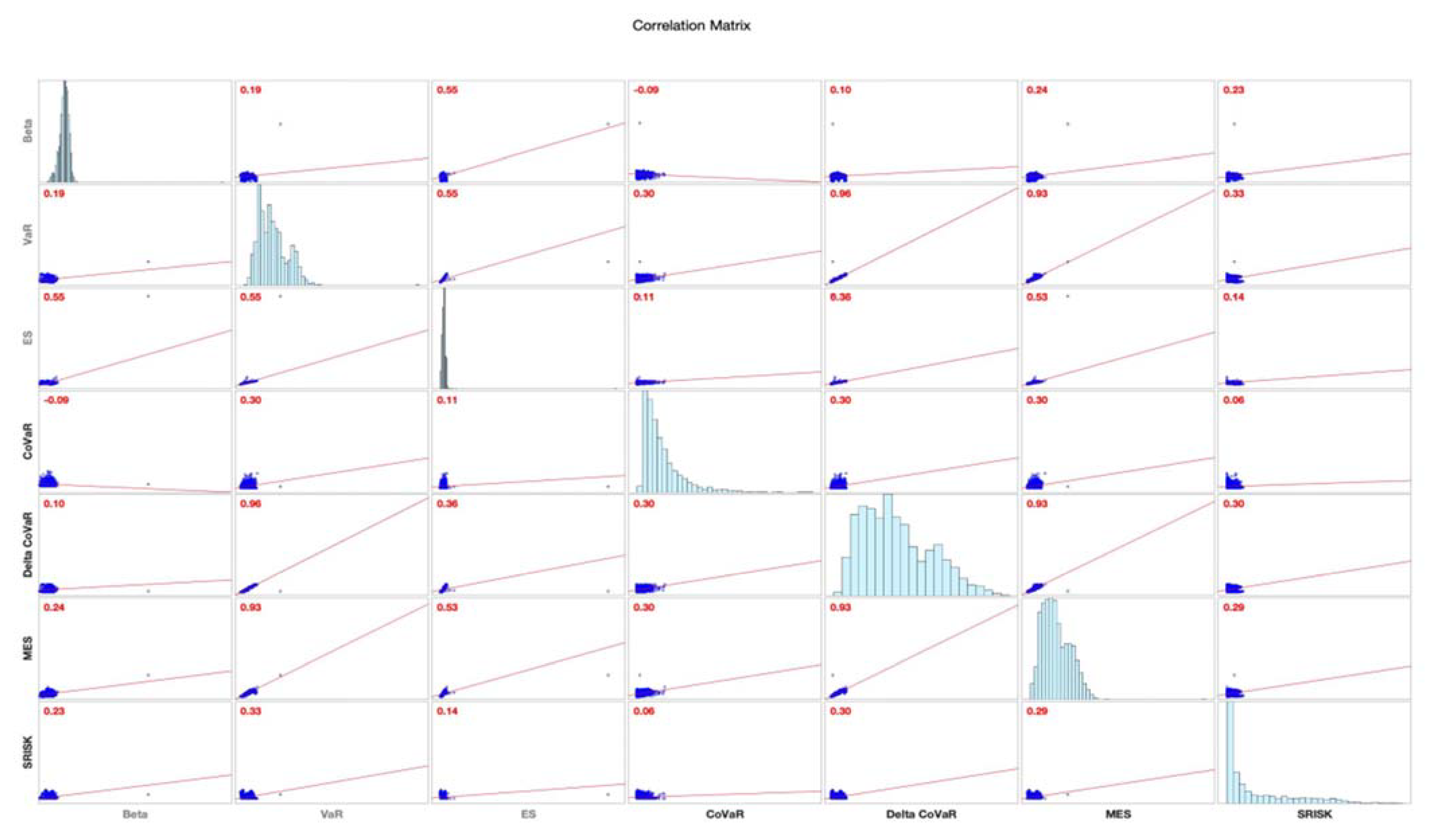
The preliminary data process involves sorting and adjusting the data composition where the statistics summary of the data is displayed in

Table 3. Descriptive Statistics.

	N	Mean	Min	Max	SD	Variance	Kurtosis
Beta	50,328	0.631	−3.821	6.539	0.572	0.327	6.614
DCOVAR	50,328	0	0.000	0	0	0	5.983
MES	50,328	0.014	0.000	0.117	0.01	0	5.954
SRISK	50,328	7.32 × 105	0.000	3.61 × 107	2.41 × 106	5.82 × 1012	47.347
EXC RATE	50,328	1.27 × 104	9.45 × 103	1.52 × 104	1.52 × 103	2.33 × 106	2.796
FFR	50,328	6.078	4.250	7.75	1.159	1.343	1.633
TBILL DELTA	50,328	−0.004	−65.220	67.33	13.029	169.746	6.188
JKSE VIX	50,328	10.407	0.010	92.02	10.346	107.047	10.39
LIQ SPR	50,328	1.244	−0.110	3.13	0.591	0.349	2.91
TED SPR	50,328	4.443	1.900	6.54	1.186	1.406	1.783

. The pairwise correlation between variables was also analysed and exhibited in

Table 4. Pairwise Correlation.

Variables	(1)	(2)	(3)	(4)	(5)	(6)	(7)	(8)	(9)	(10)	(11)	(12)	(13)	(14)
(1) Beta	1.000
(2) COVAR	−0.045 *	1.000
	(0.000)
(3) DCOVAR	0.678 *	0.030 *	1.000
	(0.000)	(0.000)
(4) MES	0.848 *	0.071 *	0.644 *	1.000
	(0.000)	(0.000)	(0.000)
(5) SRISK	0.478 *	−0.012 *	0.335 *	0.358 *	1.000
	(0.000)	(0.005)	(0.000)	(0.000)
(6) DCOVAR_1	0.040 *	0.007	0.022 *	0.076 *	0.005	1.000
	(0.000)	(0.108)	(0.000)	(0.000)	(0.292)
(7) MES_1	−0.003	0.003	−0.014 *	0.001	−0.006	0.181 *	1.000
	(0.559)	(0.465)	(0.001)	(0.811)	(0.160)	(0.000)
(8) SRISK_1	0.005	−0.004	0.000	0.004	0.003	0.008	0.002	1.000
	(0.295)	(0.343)	(0.967)	(0.406)	(0.537)	(0.057)	(0.696)
(9) EXC_RATE	0.050 *	−0.060 *	−0.006	0.041 *	0.146 *	0.005	0.004	0.006	1.000
	(0.000)	(0.000)	(0.149)	(0.000)	(0.000)	(0.262)	(0.361)	(0.181)
(10) FFR	−0.025 *	0.113 *	0.017 *	0.082 *	−0.015 *	−0.004	−0.001	−0.007	−0.205 *	1.000
	(0.000)	(0.000)	(0.000)	(0.000)	(0.001)	(0.375)	(0.844)	(0.123)	(0.000)
(11) TBILL_DELTA	0.001	−0.015 *	0.001	0.006	0.000	0.009 *	0.002	0.004	0.000	−0.002	1.000
	(0.899)	(0.001)	(0.739)	(0.201)	(0.943)	(0.040)	(0.649)	(0.328)	(0.970)	(0.664)
(12) JKSE_VIX	−0.058 *	0.162 *	0.039 *	0.100 *	−0.021 *	−0.007	−0.002	−0.004	−0.057 *	0.119 *	−0.630 *	1.000
	(0.000)	(0.000)	(0.000)	(0.000)	(0.000)	(0.127)	(0.632)	(0.320)	(0.000)	(0.000)	(0.000)
(13) LIQ_SPR	0.031 *	−0.005	0.009 *	0.060 *	0.030 *	−0.002	0.000	0.000	0.249 *	0.340 *	−0.011 *	0.014 *	1.000
	(0.000)	(0.311)	(0.042)	(0.000)	(0.000)	(0.600)	(0.951)	(0.952)	(0.000)	(0.000)	(0.012)	(0.002)
(14) TED_SPR	−0.013 *	0.107 *	0.019 *	0.094 *	−0.040 *	−0.002	−0.003	−0.008	−0.252 *	0.818 *	0.004	0.105 *	0.208 *	1.000
	(0.004)	(0.000)	(0.000)	(0.000)	(0.000)	(0.732)	(0.457)	(0.089)	(0.000)	(0.000)	(0.388)	(0.000)	(0.000)

* p < 0.1.

.

The correlation matrix for all models in Figure 1 reveal the highest correlation is for VaR and $\mathsf{\Delta }\mathrm{CoVaR}$ at 0.96, followed by MES and $\mathsf{\Delta }\mathrm{CoVaR}$ at 0.93. The number conveys that SIFIs ranking shortlist association between methodology that we can expect to be the same. On the other hand, the lowest one for SRISK and MES at 0.29, while SRISK and $\mathsf{\Delta }\mathrm{CoVaR}$ correlation is 0.30.

4.2. Systemic Risk Based on Market Model

4.2.1. CoVaR

CoVaR was used to measure the financial institutions’ systemic risk contribution, as introduced by Adrian and Brunnermeier (2016). The model was developed based on VaR by Jorion (2007) and measures the most investors can lose over a certain investment horizon. Based on data analysis as shown in

Table 5. CoVaR.

Banks	2008		2009		2010		2011		2012		2013
	% to Sys	Rank	% to Sys	Rank	% to Sys	Rank	% to Sys	Rank	% to Sys	Rank	% to Sys	Rank
BCA	30.0%	2	25.4%	1	26.6%	1	21.7%	2	30.9%	1	25.1%	1
BRI	15.8%	3	9.0%	4	9.7%	4	10.1%	5	6.4%	6	10.7%	3
BMRI	30.9%	1	17.0%	2	19.7%	2	22.4%	1	16.9%	2	22.5%	2
BNI	6.1%	4	9.2%	3	8.5%	5	10.2%	4	8.1%	4	8.7%	4
MEGA	1.1%		8.0%	5	1.8%		2.0%		2.1%		1.7%
BDMN	1.5%		1.6%		2.0%		1.7%		1.4%		2.1%
PNBN	0.9%		1.2%		1.0%		1.5%		1.1%		1.1%
BJBR	3.5%		5.7%	6	10.5%	3	10.3%	3	11.4%	3	7.3%	5
BTN	0.0%		1.2%		3.0%		2.2%		2.3%		3.1%
BSIM	0.4%		0.6%		5.0%	6	3.2%		1.2%		0.8%
BJTM	0.1%		0.1%		0.1%		0.2%		7.1%	5	6.2%	6
SDRA	1.4%		2.9%		2.1%		2.9%		2.4%		2.3%
BACA	2.1%		3.6%		3.5%		4.1%		2.6%		2.5%
AGRO	0.2%		1.1%		0.5%		0.5%		0.5%		0.6%
CCBI	1.5%		4.4%		0.7%		0.4%		0.3%		0.7%
BBKP	1.7%		2.2%		2.1%		3.2%		2.0%		2.2%
MNC	1.2%		4.3%		1.7%		2.1%		1.8%		1.0%
Others—10 banks	1.5%		2.5%		1.3%		1.3%		1.3%		1.5%
Banks	2014		2015		2016		2017		2018		2019
	% to Sys	Rank	% to Sys	Rank	% to Sys	Rank	% to Sys	Rank	% to Sys	Rank	% to Sys	Rank
BCA	19.0%	2	24.7%	1	14.9%	3	20.1%	1	20.6%	1	19.7%	1
BRI	9.9%	4	11.3%	3	7.0%	5	9.3%	5	7.9%	5	7.5%	5
BMRI	19.4%	1	20.9%	2	14.0%	4	16.9%	2	18.9%	2	15.2%	3
BNI	11.4%	3	8.6%	5	6.7%	6	10.5%	3	10.2%	4	9.6%	4
MEGA	2.2%		1.6%		1.3%		3.2%		2.4%		1.9%
BDMN	2.0%		1.9%		1.3%		3.7%		1.8%		1.8%
PNBN	1.4%		1.1%		0.9%		1.3%		1.6%		1.4%
BJBR	9.7%	5	8.9%	4	23.5%	1	9.4%	4	11.9%	3	16.9%	2
BTN	2.9%		1.4%		2.6%		2.2%		3.2%		2.5%
BSIM	1.5%		1.4%		0.8%		5.0%		2.5%		2.6%
BJTM	7.9%	6	6.3%	6	17.2%	2	6.5%	6	7.0%	6	6.0%	6
SDRA	2.8%		2.2%		1.7%		2.6%		3.3%		5.7%	7
BACA	3.4%		3.2%		1.9%		2.8%		3.4%		2.5%
BBKP	2.3%		1.8%		2.3%		2.6%		2.5%		2.7%
MNC	1.3%		1.2%		1.1%		1.0%		0.8%		0.8%
Others—12 banks	2.9%		3.5%		2.6%		2.8%		2.2%		3.1%

Source: Salim and Daly (2021).

, CoVaR SIBs rankings over the sample window time are dominated by KBMI 4 or big banks where Indonesia regulator classified them as banks with capital of more than Rp 70 trillion. They represent major players in the Indonesian banking market with more products and services offered to customers.

4.2.2. Marginal Expected Shortfall (MES)

MES, as proposed by Acharya et al. (2017), ranked banks based on their systemic contribution, which are shown in

Table 6. Marginal expected shortfall.

Banks	2008		2009		2010		2011		2012		2013
	% to Sys	Rank	% to Sys	Rank	% to Sys	Rank	% to Sys	Rank	% to Sys	Rank	% to Sys	Rank
BCA	10.77%	3	8.00%	4	7.12%	5	5.29%	8	9.79%	1	6.77%	6
BRI	16.51%	1	6.99%	6	8.00%	2	6.52%	6	5.62%	7	8.45%	2
BMRI	15.55%	2	7.50%	5	8.33%	1	7.06%	5	7.76%	3	7.75%	3
BNI	9.88%	4	13.02%	1	6.89%	6	10.18%	1	1.20%		10.51%	1
BDMN	6.67%	6	6.77%	7	7.75%	3	4.56%		6.50%	5	6.93%	4
PNBN	8.37%	5	6.60%	9	6.74%	7	8.01%	2	9.74%	2	6.91%	5
BTPN	1.20%		5.10%	11	3.31%		5.77%	7	4.05%		4.23%
Maybank	1.38%		5.01%	12	3.61%		4.16%		3.34%		2.56%
BJBR	0.64%		0.95%		6.42%	8	4.99%		5.80%	6	3.14%
BTN	0.09%		2.92%		7.63%	4	4.65%		4.28%		5.77%	7
BSIM	0.19%		0.28%		−0.45%		7.63%	3	2.57%		0.71%
SDRA	4.41%		5.81%	10	4.56%		5.28%	9	3.80%		3.89%
AGRO	2.83%		6.79%	7	3.41%		2.41%		3.92%		2.18%
BBKP	5.66%	7	6.77%	8	5.32%	9	7.17%	4	7.00%	4	5.22%	8
MNC	2.44%		9.24%	2	1.19%		0.07%		3.45%		3.78%
BAG	0.98%		4.98%		3.59%		5.16%	10	1.78%		2.08%
BNBA	3.94%		3.47%		2.11%		2.27%		2.25%		1.65%
BVIC	3.47%		8.75%	3	3.38%		3.88%		4.45%		4.00%
Others—9 banks	8.92%		−5.51%		13.17%		7.22%		13.43%		12.30%
Banks	2014		2015		2016		2017		2018		2019
	% to Sys	Rank	% to Sys	Rank	% to Sys	Rank	% to Sys	Rank	% to Sys	Rank	% to Sys	Rank
BCA	5.27%	7	7.49%	4	4.07%		6.27%	4	4.45%		5.21%	9
BRI	7.90%	2	9.89%	2	6.01%	6	8.14%	3	6.36%	6	5.77%	7
BMRI	7.02%	3	8.72%	3	5.58%	8	5.83%	6	7.33%	3	5.50%	8
BNI	12.10%	1	10.80%	1	8.33%	1	12.23%	2	11.22%	1	10.36%	2
MEGA	1.93%		1.39%		0.48%		6.16%	5	3.07%		2.04%
BDMN	6.75%	4	6.69%	5	6.03%	5	17.08%	1	6.83%	5	6.05%	5
PNBN	6.54%	5	5.14%	8	4.94%		1.81%		5.99%	7	6.88%	4
BTPN	3.84%		2.63%		1.97%		3.96%		3.70%		3.91%
BJBR	4.68%		4.75%		5.10%	9	−0.61%		2.61%		−0.28%
BTN	6.43%	6	3.10%		7.27%	3	3.04%		8.08%	2	5.21%	10
BJTM	2.57%		3.19%		7.01%	4	0.73%		1.91%		1.79%
SDRA	4.12%		2.65%		2.03%		2.79%		1.97%		3.92%
BACA	1.62%		5.18%	7	4.12%		2.38%		2.55%		2.17%
BNGA	2.55%		1.67%		3.20%		2.26%		3.69%		3.95%
AGRO	3.25%		3.16%		7.94%	2	3.85%		3.46%		8.88%	3
BBKP	4.96%		4.13%		5.78%	7	5.06%	7	5.95%	8	5.82%	6
MNC	3.73%		5.65%	6	4.15%		2.55%		1.31%		1.35%
BVIC	2.10%		4.04%		2.92%		3.89%		6.96%	4	12.75%	1
Others—9 banks	12.64%		9.71%		13.06%		12.60%		12.56%		8.70%

Source: Salim and Daly (2021).

. As we can see, it shortlisted more banks than CoVaR. The ranking movement is also noticeable when compared with the other two theoretical models. The volatility brings difficulties to bank supervisors as they need to calculate the systemic capital charge and capital injection takes time to examine before getting approval. Referring to the same table, the KBMI 4 bank still contributes mostly to Indonesia systemic risk exposure.

4.2.3. SRISK

Brownlees and Engle (2017) introduced the SRISK by integrating bank size and degree of leverage. The total SRISK shows the total amount of capital shortage shareholders need to provide or inject during the period of crisis. If the banks SRISK score is zero they have enough capital to escape the crisis, where the market decline is assumed at 40%, and the prudential capital threshold at 8%.

Table 7. SRISK.

Banks	2008		2009		2010		2011		2012		2013
	% to Sys	Rank	% to Sys	Rank	% to Sys	Rank	% to Sys	Rank	% to Sys	Rank	% to Sys	Rank
BMRI	31.14%	1	0.00%		0.00%		0.00%		0.00%		0.00%
BNI	29.17%	2	16.13%	3	0.00%		7.43%	3	0.00%		39.87%	1
BNLI	11.30%	4	24.24%	2	31.85%	2	27.93%	2	0.00%		0.00%
PNBN	0.00%		0.00%		0.00%		2.47%		70.17%	1	22.02%	3
BNGA	24.61%	3	44.70%	1	67.64%	1	49.54%	1	0.00%		0.00%
BJBR	0.00%		13.67%	4	0.00%		0.00%		3.83%		0.00%
BTN	0.00%		0.00%		0.00%		0.00%		0.00%		26.72%	2
BJTM	0.00%		0.00%		0.00%		5.75%	4	0.00%		0.00%
BBKP	2.81%		0.00%		0.00%		4.04%		18.48%	2	4.55%
BAG	0.88%		1.26%		0.51%		2.45%		1.95%		2.56%
BVIC	0.00%		0.00%		0.00%		0.39%		5.57%	3	4.29%
OTHERS—16 BANKS	0.00%		0.00%		0.00%		0.00%		0.00%		0.00%
Banks	2014		2015		2016		2017		2018		2019
	% to Sys	Rank	% to Sys	Rank	% to Sys	Rank	% to Sys	Rank	% to Sys	Rank	% to Sys	Rank
BNI	0.00%		23.91%	2	26.65%	2	26.11%	2	40.78%	1	49.14%	1
BNGA	19.62%	2	26.94%	1	12.77%	4	0.00%		11.45%	4	10.52%	4
BTPN	0.00%		0.00%		0.00%		0.00%		0.00%		1.97%
Maybank	0.00%		7.52%	5	0.00%		0.00%		0.26%		1.44%
BJBR	16.16%	3	10.77%	4	0.00%		0.00%		0.00%		0.00%
BTN	43.27%	1	13.48%	3	28.09%	1	0.00%		28.55%	2	20.15%	2
BBKP	1.84%		6.62%	6	13.36%	3	52.75%	1	13.36%	3	10.94%	3
BAG	9.18%	4	5.30%	7	3.81%		14.51%	3	2.38%		1.79%
BNBA	0.93%		0.32%		0.46%		0.00%		0.00%		0.00%
BVIC	8.19%	5	5.13%	8	4.37%		6.63%	4	3.22%		3.35%
BACA	0.81%		0.00%		0.58%		0.00%		0.00%		0.00%
AGRO	0.00%		0.00%		0.00%		0.00%		0.00%		0.70%
PNBN	0.00%		0.00%		9.90%		0.00%		0.00%		0.00%
OTHERS—14 BANKS	0.00%		0.00%		0.00%		0.00%		0.00%		0.00%

Source: Salim and Daly (2021).

exhibit SRISK estimation results are as follows:

To capture the macroeconomics market impacts to individual banks we calculate the stock beta for each entity as exhibited in the

Table 8. Beta of sample groups (2012–2019).

		Mean	Max	Min	St.Dev	Kurtosis	Skewness
2012	KBMI 4	1.175	1.571	0.803	0.177	−0.724	−0.162
	KBMI 3	0.578	0.664	0.484	0.043	−0.698	0.161
	KBMI 2	0.588	0.880	0.440	0.087	0.728	0.928
	KBMI 1	0.325	0.617	0.202	0.063	3.372	0.945
2013	KBMI 4	1.214	1.765	0.718	0.228	−0.664	0.347
	KBMI 3	0.510	0.841	0.317	0.113	0.231	0.756
	KBMI 2	0.507	0.907	0.216	0.149	0.162	0.268
	KBMI 1	0.248	0.456	0.145	0.060	0.861	1.101
2014	KBMI 4	1.715	2.356	1.419	0.163	0.723	0.528
	KBMI 3	0.560	0.763	0.395	0.080	−0.678	−0.101
	KBMI 2	0.538	0.794	0.410	0.061	0.854	0.493
	KBMI 1	0.332	0.584	0.181	0.064	0.477	0.323
2015	KBMI 4	1.463	1.855	1.061	0.160	−0.342	−0.358
	KBMI 3	0.495	0.753	0.277	0.081	−0.013	0.204
	KBMI 2	0.447	0.761	0.267	0.089	0.328	0.496
	KBMI 1	0.343	0.629	0.173	0.086	0.214	0.628
2016	KBMI 4	1.446	1.893	0.987	0.206	−0.742	0.059
	KBMI 3	0.602	1.137	0.388	0.125	1.399	0.831
	KBMI 2	0.569	1.360	0.315	0.156	4.291	1.696
	KBMI 1	0.452	1.248	0.200	0.165	5.292	1.917
2017	KBMI 4	1.506	1.845	1.116	0.154	−0.377	−0.324
	KBMI 3	0.658	1.260	0.018	0.165	3.426	−0.653
	KBMI 2	0.560	1.116	0.022	0.177	2.134	−0.533
	KBMI 1	0.550	0.994	0.240	0.139	0.604	0.766
2018	KBMI 4	1.390	1.825	0.631	0.240	1.738	−1.151
	KBMI 3	0.511	0.810	0.117	0.103	3.205	−1.402
	KBMI 2	0.322	0.604	0.098	0.099	−0.230	0.361
	KBMI 1	0.363	0.509	0.200	0.065	−0.674	−0.210
2019	KBMI 4	1.596	1.959	1.170	0.145	−0.210	−0.542
	KBMI 3	0.704	1.048	0.462	0.115	−0.009	0.515
	KBMI 2	0.609	1.430	0.375	0.126	7.732	1.466
	KBMI 1	0.418	0.637	0.300	0.071	−0.217	0.651

. Stock beta represents the likelihood of stock volatility to the benchmark index. As we can see the KBMI 4 banks group possess higher beta in all sample window. On average the beta was above 1 convey that the group more volatile compared to the JKSE index. On the opposite the other banks groups beta means less than 1 reflect the shareholders of these banks will suffer 0.3–0.5 less volatile than the overall market. We noted the volatility decreasing as the banks products and activities varies among the bank groups. OJK (2016) segregate the banking activities in Indonesia based on its capital where the tier from top KBMI 4 goes down up to KBMI 1 as the basic activities. The volatile capital market in Indonesia during the 2014 as the impact of uncertainties on Federal Reserve quantitative easing and tapering off that impact emerging economies. For more details explanation and extensive discussion of the market model results please refer to Salim and Daly (2021)

4.3. Regression Results

To test macroeconomics variables to systemic risk we employ the equation used by de Mendonça and Silva (2018) and adjusted it to reflect our specific variables:

ΔCoVaR = βΔCoVaR_t−1 + βBETA + βEXC_R + βFFR +βTBILL + βJKSEVIX + βLIQSPR + βTEDSPR + ε
MES = βMES_t−1 + βBETA + βEXC_R + βFFR + βΔTBILL + βJKSEVIX + βLIQSPR + βTEDSPR + ε
SRISK = βSRISK_t−1 + βBETA + βEXC_R + βFFR + βΔTBILL + βJKSEVIX + βLIQSPR + βTEDSPR + ε

note that,

ΔCoVaR_t−1, MES_t−1, SRISK_t−1 = ΔCoVaR, MES, and SRISK of bank t at t – 1;

BETA = bank stock beta;

EXC_R = exchange rate;

FFR = central bank funding rate;

TBILL = 3-month T bill rate;

JKSEVIX = Jakarta Stock Exchange volatility index;

LIQSPR = Liquidity spread. The difference of 3-month repo and 3-month T bill rate;

TEDSPR = TED spread. The difference of 3-month USD LIBOR and 3-month T bill rate.

Based on balanced panel data over daily observations of more than 50,000 variables the analysis executes using the fixed effects, random effects generalized least square (GLS), and random effects maximum likelihood estimator (MLE) models. The summary of estimation value is presented in

Table 9. Fixed and Mixed Effect Results Summary.

.	Panel A. DCoVaR			Panel B. MES			Panel C. SRISK
	(1)	(2)	(3)	(4)	(5)	(6)	(7)	(8)	(9)
	FE FE_DCoVaR	RE GLS RE.GLS_DCoVaR	RE MLS RE.MLS_DCoVaR	FE FE_MES	RE GLS RE.GLS_DCoVaR	RE MLS RE.MLS_DCoVaR	FE FE_MES	RE GLS RE.GLS_DCoVaR	RE MLS RE.MLS_DCoVaR
DCOVAR_1	0 ***	0 ***	0
	(23.99)	(23.96)	(−0.7)
MES_1	-	-	-	0 ***	0 ***	0 ***
				(5.56)	(5.56)	(5.56)
SRISK_1	-	-	-	-	-	-	−0.01	−0.01	−0.01
							(−0.71)	(−0.71)	(−0.71)
Beta	0 ***	0 ***	0	0.02***	0.02 ***	0.02 ***	20.50 ***	20.49 ***	20.49 ***
	(55.49)	(55.62)		(253.85)	(254.34)	(254.35)	(88.44)	(88.52)	(88.53)
EXC_RATE	0 ***	0 ***	0 ***	0 ***	0 ***	0 ***	0 ***	0 ***	0 ***
	(−5.05)	(−5.05)	(−13.46)	(16.74)	(16.74)	(16.74)	(38.97)	(38.97)	(38.98)
FFR	0	0	0 ***	0 ***	0 ***	0 ***	1.91 ***	1.91 ***	1.91 ***
	(0.47)	(0.48)	(8.86)	(9.7)	(9.7)	(9.7)	(16.12)	(16.12)	(16.12)
TBILL_DELTA	0 ***	0 ***	0 ***	0 ***	0 ***	0 ***	0.02 ***	0.02 ***	0.02 ***
	(30.6)	(30.59)	(33.44)	(63.62)	(63.62)	(63.63)	(3.28)	(3.28)	(3.28)
JKSE_VIX	0 ***	0 ***	0 ***	0 ***	0 ***	0 ***	0.05 ***	0.05 ***	0.05 ***
	(46.88)	(46.87)	(52.02)	(96.6)	(96.6)	(96.61)	(5.09)	(5.09)	(5.09)
LIQ_SPR	0 ***	0 ***	0 ***	0	0	0	−1.41 ***	−1.41 ***	−1.41 ***
	(3.05)	(3.04)	(−6.21)	(−0.01)	(−0.01)	(−0.01)	(−9.82)	(−9.82)	(−9.82)
TED_SPR	0 ***	0 ***	0 ***	0 ***	0 ***	0 ***	−0.14 ***	−1.44 ***	−1.43 ***
	(4.28)	(4.27)	(−4.45)	(18.03)	(18.03)	(18.03)	(−12.94)	(−12.94)	(−12.94)
_cons	0 ***	0 ***	0	−0.01 ***	−0.01 ***	−0.01 ***	−36.28 ***	−36.28 ***	−36.28 ***
	(33.58)	(5.35)	(−0.4)	(−23.75)	(−10.48)	(−10.32)	(−41.87)	(−13.5)	(−14.06)
Observations	50327	50327	50327	50327	50327	50327	50327	50327	50327
R-squared	0.1	0.1		0.59	0.59		0.17	0.17

t-values are in parentheses. *** p < 0.01. Panel A: DCovaR, Panel B: MES, Panel C: For SRISK coefficient are in exponent xe05.

. To check best fit model, we run the Hausman test where the outcome of Ho is statistically significant at 0.002 for ΔCoVaR reflects the random effect is consistent. On the other hand, using the same test we fail to reject Ho for MES at 0.993 and SRISK at 1 infer to choose the fixed effects model over the random effects (

Table 10. Hausman specification test.

(DCoVaR)
	Coef.
Chi-square test value	24.406
p-value	0.002
(MES)
	Coef.
Chi-square test value	1.089
p-value	0.993
(SRISK)
	Coef.
Chi-square test value	0.027
p-value	1

). The outcome of SRISK raise question and suspicious because of highly correlated of ε with the regressor. However, refer to the Section 4.2.3 remember that the Indonesia banks have enough capital even during crisis reflected in SRISK = 0 which read as autocorrelation existence in the calculation. Further, for ΔCoVaR employs Breusch Pagan Lagrangian test as displayed in

Table 11. Breusch Pagan test. Breusch and Pagan Lagrangian multiplier test for random effects.

DCOVAR[ID,t] = Xb + u[ID] + e[ID,t]
Estimated Results:
	Var	SD = sqrt(Var)
DCOVAR	6.32 × 10−13	7.95 × 10−7
E	4.83 × 10−14	2.20 × 10−7
u	1.34 × 10−13	3.66 × 10−7
Test: Var(u) = 0
	chibar2(01)	=2.1 × 107
	Prob > chibar2	=0.0000

. for random effect reject the Ho with consequences to run the pooled OLS.

As proven by the Breusch Pagan Lagrangian test, for we should run the pooled OLS for the ΔCoVaR. To choose the most robust model, the first step is to check that the assumptions of the Ordinary Least Square (OLS) hold. Stata results detected heteroscedasticity, autocorrelation, non-normality distribution of error terms (see Appendix A). Therefore, to fix the above problems, we fit the ARCH(1) and GARCH(1) models to avoid bias on estimation. The test of OLS assumptions is available in the Appendix A.

The estimation results of the ARCH(1,1) and GARCH(1,1) models for ΔCoVaR are presented in the

Table 12. CoVaR ARCH(1,1) GARCH(1,1).

Delta_CoVaR	Coef.	Std. Err.	t-Value	p-Value	[95% Conf	Interval]
Delta_CoVaR
DCovar_1	−15,697.014	2877.322	−5.46	0	−21,336.462	−10,057.566
Beta	88.335	12.162	7.26	0	64.498	112.171
Exch_Rate	0.069	0.002	33.07	0	0.065	0.073
FFR	−59.711	4.458	−13.39	0	−68.448	−50.974
TBILL_DELTA	0.648	0.156	4.14	0	0.341	0.954
JKSE_VIX	1.421	0.21	6.75	0	1.009	1.834
LIQUIDITY_SPREAD	19.918	6.29	3.17	0.002	7.589	32.247
TED_SPREAD	7.812	2.941	2.66	0.008	2.048	13.576
Constant	237.717	30.951	7.68	0	177.054	298.381
ARCH
arch
L1	0.047	0.012	3.96	0	0.023	0.07
garch
L1	0.955	0.011	85.70	0	0.933	0.976
Constant	8.457	9.509	0.89	0.374	−10.18	27.095

.

GARCH results for ΔCoVaR exhibit that all variables have a positive relationship and were statistically significant to the systemic risk escalation except for the central bank funding rate. The connection hints to how the monetary policy, through increasing or lowering interest rates, could enable systemic crises to occur. Referring to the same table, the bank stock beta and liquidity spread are the two biggest contributors precipitating the contagion effect. The bank beta indicates how the institutions’ equity behave across time with regards to the market volatility, whereas liquidity spread is an indicator of a market under distress when the spread widens during the financial crises.

To consider the effects of unobserved variables on the independent variables in ΔCoVaR, MES, and SRISK, we estimated the extension of analysis and incorporated the Finite Mixture Model (FFM). The summary of FMM class 1 and class 2 and the difference analysis for ΔCoVaR and MES is exhibited in

Table 13. Latent class marginal means.

	Coefficient	Std. Err.	t-Value	p-Value	[95% Conf	Interval]
DCOVAR	2.82 × 10−7	1.83 × 10−9	153.92	0	2.78 × 10−7	2.86 × 10−7
DCOVAR	1.08 × 10−6	1.18 × 10−8	91.64	0	1.05 × 10−6	1.10 × 10−6
MES	0.0129582	0.0000196	662.66	0	0.0129199	0.0129966
MES	0.0173357	0.0000992	174.72	0	0.0171413	0.0175302

. For SRISK, the FMM fails to achieve the convergence, and it was concluded that it is best to stick to the fixed model.

Based on the regression, overall output and the outcome can be summarized as follow:

• Beta and market index volatility: Stock beta have a positive correlation and are statistically significant to the systemic risk in all market model estimations. In this case, the bank systemic risk swings downward or upward in the same direction as the overall market. The results also confirmed that we applied market index volatility. The investigation of using simple beta to sort the systemic bank was also suggested by Benoit et al. (2013).
• Exchange rate: The fluctuation of exchange rate could trigger and amplify the systemic risk in the economy. Its effects statistically significantly validated both the linear and ARCH models. Our findings were similar to Yesin (2013), Mayordomo et al. (2014), and de Mendonça and Silva (2018). However, they were contrary to Tram and Thi Thanh Hoai (2021). The shock of exchange rate volatility influence the banks’ assets and liabilities, especially when there is no hedging or insurance to cover the risk. The Asia Financial Crises in 1997, where Indonesia was one of severely hit economies, is a good example of the catastrophic impact of exchange rate to the banking system.
• Central bank funding and T bill rate: The outcome is statistically significant, while the effect was mixed between estimation models. CoVaR and MES reported the negative effects of FFR on the systemic risk, while SRISK reported the opposite. We suspect that the SRISK methodology, which considered the leverage effect, the outcome where bank assets sensitivity to the monetary policy interest rate changes, which was also studied by Jobst (2014) and Brunnermeier and Pedersen (2009). From another perspective, when we assessed the delta of the 3-month T bill, the implication was the same across all models. The phenomena could indicate that the banks are more sensitive to the FFR than the 3-month T bill rate, as it resembles the overnight money market of short-term liquidity resorts. Ramos-Tallada (2015) also iterated the sensitivity of banks to short-term interest rates and potential losses during the tight monetary policy.
• Liquidity spread: In general, the liquidity spread is not significantly related to the banks’ systemic risk exposure. Because we used the 3-month repo rate, the non-existence could be traced to the very limited repo transactions in the Indonesian banking market. However, the effect could be different for other countries as it very much depends on the banks’ portfolios. On the other hand, TED spread the results are quite mixed among models. CoVaR detected a negative trend for systemic risk and was in line with Ramos-Tallada (2015), while MES and SRISK perceived the change as adding more fuel to the risk (Laséen et al. 2017). Further research should explore the impact of the SRISK model on benchmark rates as it is also arguably in line with the central bank and funding rate.

4.4. Technical Integration

The BCBS (2018) indicator-based approach values the institution size, interconnectedness, substitutability, global cross-jurisdictional activity, and complexity. Basel guidelines give an equal proportion of 20% weight to the five categories. BCBS (2012) allows departure from the guidelines with purpose to better capture specific Domestic Systemically Important Banks (D-SIBs) characters and country externalities. Indonesia Financial Services Authority (OJK) as the bank regulator adjusted the formula composition and re-arranged the indicators following POJK No. 2/POJK.03/2018. The SIBs assessment indicators after country adjustment are exhibited in

Table 14. Basel and OJK Indicators.

Category and Weighting	BCBS G-SIBs	Indicator Weighting	Category (Weighting)	Adjusted Indicators D-SIBs	Indicator Weighting
Size (20%)	Total exposures	20%	Size (33.3%)	Total exposures	100%
Interconnectedness (20%)	Intra-financial system assets	6.67%	Interconnectedness (33.3%)	Intra-financial system assets	33.3%
	Intra-financial system liabilities	6.67%		Intra-financial system liabilities	33.3%
	Securities outstanding	6.67%		Securities outstanding	33.3%
Complexity (20%)	Notional amount of over the counter (OTC) derivatives	6.67%	Complexity (33.3%)	Notional amount of over the counter (OTC) derivatives	25%
	Level 3 assets	6.67%		Trading and available-for-sale securities	25%
	Trading and available for sale securities	6.67%		Domestic indicators	25%
				Substitutability (payment system & custodian)	25%
Substitutability (20%)	Assets under custody	6.67%
	Payment activity	6.67%
	Underwritten transactions in debt & equity markets	3.33%
	Trading volume	3.33%
Cross-jurisdictional activity (20%)	Cross-jurisdictional claims	10%
	Cross-jurisdictional liabilities	10%

Source: OJK (2018).

.

We aimed to provide a practical assessment framework and possible technical indicators to integrate the effects of macroeconomic shocks into the SIBs calculation. The tailor-made designs for each country were not only permitted by Basel but were also important for providing holistic supervision analysis to mitigate future systemic risk (BCBS 2012). We used Indonesian banks as the sample, but regulatory authority could be replicated to non-bank financial institutions, albeit adjusted to industry or specific country characteristics, risk, etc. The framework starts using a base model derived from BCBS (2018) and is then developed using a combination of macroeconomics and micro-bank granular data. During the preliminary steps, supervisors discuss what variables or ratios to use that represent both aspects and allocate weight to each variable and what technical computation methods and data sources to use. Some reading related to the specific country SIBs like Brämer and Gischer (2013) when determining the suggestion for Australia D-SIBs, Bengtsson et al. (2013) for Sweden banks, and Glasserman and Loudis (2015) in their report comparing the US and international G-SIBs.

The third step involved the data collection process, where much varies depending on what statistics are gathered. The source could come from the internal data warehouse based on financial report submissions or external database sources. After data collection, the process continues to the analysis and technical calculations. For thorough assessment processes, we propose the integration of the market model approach to complement and validate the systemic bank shortlist based on Basel. The choice of market model could also be developed further to suit policy-makers’ needs. Regarding the weight for each ratio or parameters, they could be attributed equally or based on some other methods, such as using structural equation model, professional judgment and survey, or a combination of both. The last step in the framework is to group the banks or financial institutions based on the analysis. The methods for segregating the groups are also quite open, which can act as a validation tool for comparison. For the illustration of framework refer to Figure 2.

In addition, to put the assessment framework into practice or technical calculation, we also suggest adding some ratios and parameters to reflect the integration of macro and micro data into the SIBs calculation (see

Table 15. SIBs Technical Integration.

Category and Weighting	BCBS G-SIBs	Indicator Weighting	Category (Weighting)	POJK No. 2/POJK.03/2018 Indicators D-SIBs		Indicator Weighting	Category (Weighting)	Macro-Micro Indicators D-SIBs	Indicator Weighting
Size (20%)	Total exposures	20%	Size (33.3%)	Total exposures		100%	Size (25%)	Total exposures	100%
Interconnectedness (20%)	Intra-financial system assets	6.67%	Interconnectedness (33.3%)	Intra-financial system assets		33.3%	Interconnectedness (25%)	Intra-financial system assets	33.3%
	Intra-financial system liabilities	6.67%		Intra-financial system liabilities		33.3%		Intra-financial system liabilities	33.3%
	Securities outstanding	6.67%		Securities outstanding		33.3%		Securities outstanding	33.3%
Complexity (20%)	Notional amount of over the counter (OTC) derivatives	6.67%	Complexity (33.3%)	Notional amount of over the counter (OTC) derivatives		25%	Complexity (25%)	Notional amount of over the counter (OTC) derivatives	25%
	Level 3 assets	6.67%		Trading and available-for-sale securities		25%		Trading and available-for-sale securities	25%
	Trading and available for sale securities	6.67%		Domestic indicators		25%		Domestic indicators	25%
				Substitutability (payment system & custodian)		25%		Substitutability (payment system & custodian)	25%
Substitutability (20%)	Assets under custody	6.67%					Macroeconomics shocks (25%)	Currency exposure	33.3%
	Payment activity	6.67%						Market volatility	33.3%
	Underwritten transactions in debt & equity markets	3.33%						Policies exposure	33.3%
	Trading volume	3.33%
Cross-jurisdictional activity (20%)	Cross-jurisdictional claims	10%
	Cross-jurisdictional liabilities	10%

Source: Author adapted from BCBS (2018) and OJK (2018).

). The change of methodology for the reviewing process is also encouraged by Basel at least once every three years (BCBS 2018). The proposed sample of ratios to represent macroeconomics shocks in line with our previous regression results, like currency exposures.

Incorporating the entity creates exposure to an unfavourable swing of currency movement, i.e., unhedged liabilities to total liabilities. Indonesia experienced high currency volatility during the Asia Financial Crises in 1997 after the shift from the pegged currency system to the floating system. Nowadays, the central bank imposes mandatory hedging to portion foreign liabilities; however, some are still exposed to sudden shocks.

Market volatility: Stock beta, marked to market securities per total securities in portfolio, T-bills, and T-bonds to total securities. This ratio is to acknowledge the effect of market volatility that could bring potential harm to financial institutions. We also consider government bonds risky investments, where the Eurozone sovereign debt crisis in 2010–2011 is a fine example of a similar condition. Paltalidis et al. (2015) provided evidence where the sovereign credit channel was one of the systemic risk transmission channels.

Policies exposure: The delta of future incomes or liabilities are seen as the consequences of change in the policy interest rate. The ratios aim to capture the entity fragility coming from government regulations or policy-makers’ decisions. The sample under this criterion shows the change in risk free anchor rate, people mobility restriction impact on business during the Covid pandemic, administered price, etc.

5. Conclusions and Policies Implication

This paper investigated how macroeconomic shocks could affect systemic risk through several transmission channels. To explore macroeconomic variables’ connection to systemic risk, we employed three market models: CoVaR (Adrian and Brunnermeier 2016), expected marginal shortfall (Acharya et al. 2012), and SRISK (Brownlees and Engle 2017) using the adjusted linear equation used by de Mendonça and Silva (2018) and carrying it forward by employing fixed effects, random effects, and GARCH models. To consider the unobserved groups of variables that could affect the independent variables, we fit FMM. The findings show that stock beta, market index volatility, and exchange rate volatility amplify the transmission of systemic risk. In addition, the change in anchor interest rate by policy-makers is also significantly proven by statistics, though the effect varies among the market models. The difference could come from the employed method variables and the impact being different for each interest rate time horizon. Furthermore, related to the liquidity spread, the outcomes are a mixture between models.

This paper proposes some practical improvement steps in the systemic risk assessment framework to better capture the potential macroeconomic shocks. We also suggest technical integration calculation samples and ratios reflecting the added steps. The integrated macro and micro granular data could portray the overall risk endogenously and externally expose the systemically important financial institutions.

However, the study poses some shortcomings as it does not isolate certain window periods of crises, and it applied the cross-section systemic risk models only. The limitations open the opportunity for further research to explore the impact of other non-cross section models, such as the cross-entropy joint probability of defaults and isolating the outcome to certain crises, such as the GFC 2008 and COVID-19 pandemic.

References

- Acharya, Viral, Robert Engle, and Matthew Richardson. 2012. Capital Shortfall: A New Approach to Ranking and Regulating Systemic Risks. American Economic Review 102: 59–64. [Google Scholar] [CrossRef]
- Acharya, Viral, Lasse H. Pedersen, Thomas Philippon, and Matthew Richardson. 2017. Measuring Systemic Risks. Review of Financial Studies 30: 2–47. [Google Scholar] [CrossRef]
- Adrian, Tobias, and Markus K. Brunnermeier. 2016. CoVaR. American Economic Review 106: 1705–41. Available online: https://www.aeaweb.org/articles?id=10.1257/aer.20120555 (accessed on 29 April 2019). [CrossRef]
- Akhter, Selim, and Kevin Daly. 2017. Contagion risk for Australian banks from global systemically important banks: Evidence from extreme events. Economic Modelling 63: 191–205. [Google Scholar] [CrossRef]
- Ali, Ashgar, and Kevin Daly. 2010. Macroeconomic determinants of credit risk: Recent evidence from a cross country study. International Review of Financial Analysis 19: 165–71. [Google Scholar] [CrossRef]
- BCBS. 2011. Global Systemically Important Banks: Assessment Methodology and the Additional Loss Absorbency Requirement. Basel: Bank for International Settlements. [Google Scholar]
- BCBS. 2012. A Framework for Dealing with Domestic Systemically Important Banks. Basel: Bank for International Settlements. [Google Scholar]
- BCBS. 2018. Global Systemically Important Banks: Revised Assessment Methodology and The Higher Loss Absorbency Requirement. Basel: Bank for International Settlements. [Google Scholar]
- Belluzo, Tommaso. 2020. Systemic Risk, 3.0.0 ed. GitHub. Available online: https://github.com/TommasoBelluzzo/SystemicRisk (accessed on 13 June 2019).
- Bengtsson, Elias, Ulf Holmberg, and Kristian Jonsson. 2013. Identifying systemically important banks in Sweden—What do quantitative indicators tell us? Sveriges Riksbank Economic Review 2013: 2. Available online: http://archive.riksbank.se/Documents/Rapporter/POV/2013/2013_2/rap_pov_artikel_3_130918_eng.pdf (accessed on 29 April 2019).
- Benoit, Sylvain, Gilbert Colletaz, Christophe Hurlin, and Christophe Perignon. 2013. A Theoretical and Empirical Comparison of Systemic Risk Measures: MES versus CoVaR. SSRN Electronic Journal. [Google Scholar] [CrossRef]
- Bisias, Dimitrios, Mark Flood, Andrew W. Lo, and Stavros Valavanis. 2012. A Survey of Systemic Risk Analytics. Annual Review of Financial Economics 4: 255–96. Available online: https://www.annualreviews.org/doi/abs/10.1146/annurev-financial-110311-101754 (accessed on 27 October 2018). [CrossRef]
- Brämer, Patrick, and Horst Gischer. 2013. An Assessment Methodology for Domestic Systemically Important Banks in Australia. Australian Economic Review 46: 140–59. [Google Scholar] [CrossRef]
- Brownlees, Christian, and Robert F. Engle. 2017. SRISK: A Conditional Capital Shortfall Measure of Systemic Risk. Review of Financial Studies 30: 48–79. [Google Scholar] [CrossRef]
- Brunnermeier, Markus K., and Lasse Heje Pedersen. 2009. Market Liquidity and Funding Liquidity. Review of Financial Studies 22: 2201–38. [Google Scholar] [CrossRef] [Green Version]
- De Bandt, Olivier, and Philipp Hartmann. 2000. Systemic Risk: A Survey. Working Paper No. 35. Frankfurt: European Central Bank. Available online: https://www.ecb.europa.eu/pub/pdf/scpwps/ecbwp035.pdf (accessed on 8 August 2018).
- de Mendonça, Helder Ferreira, and Rafael Bernardo da Silva. 2018. Effect of banking and macroeconomic variables on systemic risk: An application of ΔCOVAR for an emerging economy. The North American Journal of Economics and Finance 43: 141–57. [Google Scholar] [CrossRef]
- ECB. 2009. Financial Stability Review. Frankfurt: European Central Bank, pp. 134–42. Available online: https://www.ecb.europa.eu/pub/fsr/shared/pdf/ivbfinancialstabilityreview200912en.pdf?a3fef6891f874a3bd40cd00aef38c64f (accessed on 9 December 2018).
- Festić, Mejra, Alenka Kavkler, and Sebastijan Repina. 2011. The macroeconomic sources of systemic risk in the banking sectors of five new EU member states. Journal of Banking & Finance 35: 310–22. [Google Scholar] [CrossRef]
- Glasserman, Paul, and Bert Loudis. 2015. A Comparison of US and International Global Systemically Important Banks; Washington, DC: Office of Financial Research. Available online: https://www.financialresearch.gov/briefs/files/OFRbr-2015-07_A-Comparison-of-US-and-International-Global-Systemically-Important-Banks.pdf (accessed on 24 July 2021).
- Hirtle, Beverly, Anna Kovner, James Vickery, and Meru Bhanot. 2016. Assessing financial stability: The Capital and Loss Assessment under Stress Scenarios (CLASS) model. Journal of Banking & Finance 69: S35–S55. [Google Scholar] [CrossRef]
- Hollo, Dániel, Manfred Kremer, and Duca Lo. 2012. Marco CISS—A Composite Indicator of Systemic Stress in the Financial System. Frankfurt: European Central Bank (ECB). [Google Scholar]
- Illing, Mark, and Ying Liu. 2006. Measuring financial stress in a developed country: An application to Canada. Journal of Financial Stability 2: 243–65. [Google Scholar] [CrossRef]
- Jobst, A. Andreas. 2014. Measuring systemic risk-adjusted liquidity (SRL)—A model approach. Journal of Banking & Finance 45: 270–87. [Google Scholar] [CrossRef]
- Jorion, Philippe. 2007. Value at Risk: The New Benchmark for Managing Financial Risk, 3rd ed. New York: McGraw Hill. [Google Scholar]
- Laséen, Stefan, Andrea Pescatori, and Jarkko Turunen. 2017. Systemic risk: A new trade-off for monetary policy? Journal of Financial Stability 32: 70–85. [Google Scholar] [CrossRef]
- MacDonald, Ronald, Vasilios Sogiakas, and Andreas Tsopanakis. 2018. Volatility co-movements and spillover effects within the Eurozone economies: A multivariate GARCH approach using the financial stress index. Journal of International Financial Markets, Institutions and Money 52: 17–36. [Google Scholar] [CrossRef]
- Mayordomo, Sergio, Maria Rodriguez-Moreno, and Juan Ignacio Peña. 2014. Derivatives holdings and systemic risk in the U.S. banking sector. Journal of Banking & Finance 45: 84–104. [Google Scholar] [CrossRef]
- Oet, Mikhail, John Dooley, and Stephen Ong. 2015. The Financial Stress Index: Identification of Systemic Risk Conditions. Risks 3: 420–44. [Google Scholar] [CrossRef]
- OJK. 2016. Commercial Bank Activities and Business Network based on Core Capital. POJK No. 6/POJK.03/2016. Jakarta Indonesia. Available online: https://www.ojk.go.id/id/regulasi/Pages/Perubahan-POJK-Nomor-6-POJK.03-2016-tentang-Kegiatan-Usaha-dan-Jaringan-Kantor-Berdasarkan-Modal-Inti-Bank.aspx (accessed on 8 November 2019).
- OJK. 2018. Systemically Important Banks and Capital Surcharges. POJK No. 2/POJK.03/2018. Jakarta Indonesia. Available online: https://www.ojk.go.id/id/regulasi/Documents/Pages/Penetapan-Bank-Sistemik-dan-Capital-Surcharge/POJK%202-2018.pdf (accessed on 15 April 2018).
- OJK. 2021. Commercial Banks. POJK No. 12/POJK.03/2021. Jakarta Indonesia. Available online: https://www.ojk.go.id/id/regulasi/Documents/Pages/Bank-Umum/POJK%2012%20-%2003%20-2021.pdf (accessed on 12 December 2021).
- Paltalidis, Nikos, Dimitrios Gounopoulos, Renatas Kizys, and Yiannis Koutelidakis. 2015. Transmission channels of systemic risk and contagion in the European financial network. Journal of Banking & Finance 61: S36–S52. [Google Scholar] [CrossRef] [Green Version]
- Ramos-Tallada, Julio. 2015. Bank risks, monetary shocks and the credit channel in Brazil: Identification and evidence from panel data. Journal of International Money and Finance 55: 135–61. [Google Scholar] [CrossRef]
- Salim, Muhammad Zulkifli, and Kevin Daly. 2021. Modelling Systemically Important Banks vis-à-vis the Basel Prudential Guidelines. Journal of Risk and Financial Management 14: 295. [Google Scholar] [CrossRef]
- Schleer, Frauke, and Willi Semmler. 2015. Financial sector and output dynamics in the euro area: Non-linearities reconsidered. Journal of Macroeconomics 46: 235–63. [Google Scholar] [CrossRef]
- Tram, Thi, Xuan Hong, and Nguyen Thi Thanh Hoai. 2021. Effect of macroeconomic variables on systemic risk: Evidence from Vietnamese economy. Economics and Business Letters 10: 217–28. [Google Scholar] [CrossRef]
- Yesin, Pinar. 2013. Foreign Currency Loan and Systemic Risk in Europe. St. Louis: Federal Reserve Bank of St. Louis., Missouri United States, vol. 95, pp. 219–35. [Google Scholar]
Figure 1.
Correlation matrix all models.