
Cyber Insurance Premium Setting for Multi-Site Companies under Risk Correlation


1
Department of Economics, Roma Tre University, Via Silvio D’Amico 77, 00145 Rome, Italy
2
Department of Law, Economics, Politics and Modern Languages, LUMSA University, Via Marcantonio Colonna 19, 00192 Rome, Italy
*
Author to whom correspondence should be addressed.
Risks 2023, 11(10), 167; https://doi.org/10.3390/risks11100167
Submission received: 21 August 2023
/
Revised: 18 September 2023
/
Accepted: 20 September 2023
/
Published: 22 September 2023
Abstract
:Correlation in cyber risk represents an additional source of concern for utility and industrial infrastructures, where risks may be introduced by connected systems. A major means of reducing risk is to transfer it through insurance. In this paper, we consider a company which has peripheral branches in addition to its headquarters, where risk correlation is present between all of its sites and insurance is adopted to hedge against economic losses. We employ the expected utility principle (which leads to the well-known mean variance premium formula) to derive the insurance premium under risk correlation under several risk scenarios. Under a first-order approximation, a quasi-linear relationship between the premium and the two major risk factors (the number of branches and the risk correlation coefficient) is determined.
1. Introduction
Nowadays, companies face increasing risks and potential monetary losses. However, the notion of risk may be subject to different interpretations. Aven (2010); Aven and Flage (2020) have devoted significant efforts to provide the definitional foundation for the notion of risk. For example, we can consider the definition "Risk is a measure of the probability and severity of adverse effects” or the alternative “Risk is the combination of the probability of an event and its consequences” (see also Kaplan and Garrick (1981); Lowrance (1976)). An established view considers the following three major features of risk, whose combination may be employed as a synthetic description of any risk Marotta et al. (2017):
- Threat: the causes that create risks (e.g., theft of information, dangerous weather, fire);
- Vulnerability: existing weaknesses that can be exploited to cause security accidents;
- Impact: the amount of loss suffered.
An attempt to classify the levels of risk for companies and their potential consequences is reported by Aven and Cox (2016).
From the point of view of a company, the fear of monetary losses is a great incentive to implement risk management strategies and achieve economic well-being. Risk management comprises the identification, assessment, and prioritization of risks, followed by the coordination and economics-aware application of resources to minimize the probability or impact of unfortunate and unexpected events Albadarneh et al. (2015); Refsdal et al. (2015). Risk analysis and risk management are essential for companies to cope with disruption of services and the consequent economic losses Covello and Mumpower (1985); Kaplan (1991); Landsman and Sherris (2001); Paté-Cornell et al. (2018); Zio (2007). In particular, risk management may help companies in preventing or reducing the impact of several types of risks: strategic risks Frigo and Anderson (2011), financial risks Erb et al. (1996), risk of globalization Broner and Ventura (2011), and operational risks Power (2005). What is of interest to us in this paper is cyber risk, which is fast becoming the most worrying type of risk faced by companies Florackis et al. (2023). In particular, cyber risks are now seen as a major source of concern for various public utilities and industrial infrastructures due to the risk arising in individual infrastructures that derive from their interconnections and interdependencies Bürger et al. (2019); Eling (2020); Kröger (2008); Maglaras et al. (2018).
A company can devise different strategies to cope with risks. An accepted classification, which can be straightforwardly adopted for cyber risk, considers the following strategies Peterson (2020): risk avoidance, risk spreading, risk transfer, risk reduction, and risk acceptance. Excluding the first and the last strategies, which correspond, respectively, to the extreme strategies of zeroing the risk and accepting it all, the remaining strategies may be aggregated into the following two:
- Risk transfer;
- Risk mitigation.
Risk transfer consists of transferring one’s own risks to a third party. Risk mitigation is instead another name for risk reduction and includes all those activities by which the frequency and/or impact of risky events can be reduced.
A different way to cope with the problem is to invest in self-protection (a form of risk mitigation), but determining the right level of investment in cyber security is not simple Fielder et al. (2016). In addition, the costs of self-protection could be really large Armenia et al. (2021); Mazzoccoli and Naldi (2020b, 2022); Young et al. (2016). If companies decide to opt for risk transfer measures, they can purchase an insurance policy. In particular, firms may avoid most of the risks leading to economic losses by paying an insurance premium to an insurer, because the insurer will cover all the losses suffered by firms based on what is reported in the insurance policy stipulated between the insurer and the insured (see, e.g., the report by the Straub and Swiss Association of Actuaries (Zürich) (1988)).
However, the lack of statistical data about security accidents and the inaccurate knowledge of risks by the insurer may lead to overpriced insurance premiums Bandyopadhyay et al. (2009, 2010). In the literature, the topics of premium computation and principles have been addressed, e.g., by Böhme and Schwartz (2010); David (2015); Laeven and Goovaerts (2008); Lima Ramos (2017); Mastroeni et al. (2019).
A further problem arises when we consider a set of vulnerable entities whose risks are correlated. This is the case, e.g., for a company’s headquarters and its branches, where a breach in any of the entities may disclose information to breach other entities Khalili et al. (2018); Mazzoccoli and Naldi (2021); Xu et al. (2019). Though this topic has been extensively addressed in the literature, the models proposed are often complex and may not be easy to apply in an industrial context.
Our main contribution here is to build a simple mathematical model for the insurance premium that considers the risk correlation between headquarters and its branches and to show its application in a sample scenario.
The article is structured as follows. After a brief literature review in Section 2, we describe risk correlation in Section 3 and derive a formula for the insurance premium in the case of risk correlation in Section 4. The formula details are sorted out in Section 5, where we analyse the importance of choosing the aversion risk coefficient in computing the premium. We apply the formula in some reference scenarios in Section 6.
A glossary of all the terms and symbols employed in the paper is reported in Table 1 for the reader’s convenience.
2. Literature Review
In this section, we present an overview of research papers that have dealt with cyber risk correlation and the computation of insurance premiums under this scenario. We will proceed by first considering papers that have adopted simpler, model-free characterization (which is the approach we have opted for in this paper) to move later to more complex models. It is to be noted that here we refer to the correlation between victims, i.e., the probability that a potential victim suffers a breach due to another victim being breached. We do not refer to the cases of correlated risks for the same victim (i.e., the correlation between different sources of risk).
Before delving into the specific of interdependent risks, we must, however, mention some reference works that have provided a general framework for the use of insurance in cyber risk or a panorama of the different approaches taken for this purpose. We mention the works by Boehme, e.g., Böhme et al. (2019), Eling (2020), and that by Marotta et al. (2017).
Moving now to the different approaches taken to describe the interdependence of cyber risks, we can classify them according to the mathematical tool employed for this purpose, giving the following list:
- Increased breach probability;
- Correlation coefficient;
- Regression;
- Joint probability distribution function;
- Multi-dimensional stochastic process;
- Copulas.
Probably the simplest approach to describe correlation is to assume that it increases the probability of a breach, i.e., the breach probability of subject j when subject i has suffered from a breach is larger than in the reverse case. This is the approach taken by Dou et al. (2020), where the expected utility is employed to compute the premium. A logarithmic utility function is adopted. The same indirect approach to quantify correlation is adopted by Öğüt et al. (2011), where the focus is, however, not premium computation but the use of incentives to push firms into investing in self-protection. They found that subsidizing self-protection investments, rather than insurance subscriptions, helps induce companies to invest in self-protection in a socially optimum way. Quite the same approach is taken by Kunreuther and Heal (2003) (which was adopted subsequently by Hoang et al. (2017) or the case of plug-in electric vehicles), where a game model is formulated, with the probability of being breached depending on the actions of the other agents. The same model of Kunreuther and Heal (2003) is also employed by Johnson et al. (2014).
The next step up in correlation characterization complexity is to employ a correlation coefficient (which is the approach we take here). This is done, e.g., by Yang et al. (2020), where power stations are used as the infrastructure under attack. They use ruin theory to compute the premium, which is based on the loading factor formula, precisely as loading on the average amount of claims. The same approach considered here has been proposed by Xu et al. (2019) for the optimal allocation of cyber security investments for headquarters and its branches subjected to cyber risk interconnections and by Mazzoccoli and Naldi (2021) to obtain a closed formula for the optimal investment in security under a set of cyber insurance liability scenarios considering a multi-branch firm with correlated vulnerability.
A little step-up in the complexity of characterization is achieved by considering a regression model to relate the risks suffered by different agents. Lin et al. (2018) proposed a logistic regression where the following regressors are used: the number of past breaches either in the company’s supplier industries or in the company’s consumer industries, the company’s IT budget, the number of vendors of software used by the company, the standard deviation of the IT budget across sites, and a set of financial variables.
Passing now to model-based approaches, Liu et al. proposed a semi-Markov process model for attacks, where the premium is computed through the loading factor formula based on the Value-at-Risk Liu et al. (2020). A multivariate normal model is instead employed by Khalili et al. (2019), where a linear contract is considered with a discount on the base rate related to a pre-screening assessment by the insurer to reduce information asymmetry. A similar semi-Markov process is considered by Zhang et al. (2020) to model the cyberattacks against pump stations in a water distribution system. The premium is computed as the Value-at-Risk. A Stackelberg security game is proposed by Lau et al. (2020) to derive the optimal strategy to allocate defence resources against cyber attacks, modeled again by a semi-Markov process kernel. The premium is computed as the Tail-Value-at-Risk.
Some papers deal with the the interdependence of cyber risk by treating it as due to the propagation of an infection. Fahrenwaldt et al. (2018) employed the susceptible–infected–susceptible (SIS) model. Each node may be in either state (infected or susceptible). It may transition to the infected state upon influence by its neighbours and revert to the susceptible state after being cured. They used a polynomial approximation for claims to compute the aggregate expected losses, but do not provide indications about pricing. A multi-group SIR model (susceptible, infectious, or recovered) is employed by Hillairet et al. (2022) to differentiate the propagation of attacks depending on the industrial sector of the company. Again, the model allows for the computation of losses, but no approach is taken for pricing. An inhomogeneous SIS model, which also accounts for the presence of clusters where the infection propagates faster, is considered by Antonio et al. (2021). The insurance premium is said to have been computed using the utility principle and the standard deviation premium principle, but no further details are given. A multivariate risk measure introduced by Dhaene et al. (2002) is adopted by Da et al. (2021) to describe the impact of correlation in a network where a limited propagation of risk is assumed. Both the standard deviation premium principle and the variance premium principle are considered for premium computation.
Finally, the most complex characterization of correlation is probably given by copulas. A copula model is employed by Lau et al. (2021), again in the context of power stations. Premium computation is carried out by using Tail-Value-at-Risk (probably quite an extreme assessment of risk) using a coalition of insureds to reduce the premium by compensating cor extreme value occurrences. Gumbel and Clayton copulas are tested by Herath and Herath (2011) on the basis of ICSA (International Computer Security Association) data to model the correlation between the number of computers affected and the dollar value of losses. The insurance premium is computed using a very simple formula that just discounts the expected loss. Again, Gumbel and Clayton copulas, with the addition of a Frank copula, are employed in Su et al. (2021) to model the correlation between the frequency of cyber incidents and the number of computers involved. The same approach as used by Herath and Herath (2011) is taken for premium computation. A vine copula is instead proposed by Peng et al. (2018), where an ARMA-GARCH (AutoRegressive Moving Average - Generalized AutoRegressive Conditional Heteroskedasticity) model is used to describe the marginal process of individual servers under attack. No indications are provided for insurance premium computation. A mixed approach is proposed by Böhme and Kataria (2006), where a correlation coefficient is employed to describe correlation in the intra-company scenario and a t-copula is used for global correlation among the companies in the insurer’s portfolio.
3. Multi-Site Companies, Cyber Risk Correlation, and Cyber Insurance
As stated in the Introduction, we are interested in a scenario where a company has many sites (its headquarters plus several branches), all subject to cyber risk, with the levels of cyber risks experienced on the different sites being correlated. We also assume that the company intends to resort to insurance to protect itself against cyber risk on all its sites. In this section, we describe the scenario more precisely and introduce the quantities of interest to describe cyber risk and the insurance contract.
We consider a set of n sites. For the time being, we do not distinguish between the headquarters and its branches. All the mathematical treatments in the following will not make use of such a distinction. Actually, all the results stay valid if we do not consider the branches of a single company but the sites of different companies, as long as the cyber risks suffered by those companies are correlated.
The reason for cyber risk correlation may be multifarious. The sites may share portions of their databases containing information that may be used to compromise other sites, or a site may be used to launch an attack against another site, being recognized as a trustful partner and possessing credentials that allow it to penetrate the victim site’s defence lines. Examples of such situations are reported by Nagurney and Shukla (2017). Here, we do not go further into describing the security vulnerabilities that may lead to the correlation of cyber risks.
The consequence of correlation is that any site may be prone to two kinds of cyber attack Xu et al. (2019):
- Direct attack due to the attacker attempting to breach the site without exploiting information or vantage positions from another site;
- Indirect attack due to breaches that take place in another site.
As a consequence of a successful attack, the generic i-th site suffers an economic loss described by the random variable , . Each random loss follows a probability distribution (which may be different among the sites). However, for the time being, we do not make any assumption regarding the marginal distribution and assume to know just its first two moments and .
We also assume that any two losses and are correlated, their correlation being described by their covariance .
We assume that the assets owned by the company on its generic i-th site are , . These assets are threatened by attackers, which would cause the loss .
However, the value of the i-th site is mediated by the utility function
For our aims, we suppose that :
- Is a twice differentiable function on ;
- Is an increasing function and concave on .
We recall that the loss X suffered by the company on its sites is a multidimensional random variable with non-independent random variable components, which diminishes the value of each site’s asset, so that the value of the i-th site after the attack is the random quantity .
On the other hand, the company wishes to indemnify itself against cyberattacks by paying an insurance premium for its i-th site. Its utility will also be reduced to because of that payment to the insurer.
According to the expected utility principle Kaas et al. (2008), we can set a fair premium by comparing the alternatives for the insured: buying an insurance policy and ending up with utility for the i-th site, or suffering the (random) monetary loss and ending up with utility . In order to consider the problem of insurance for the set of all the sites, we define the vectors of the assets, losses, and premiums, respectively, as , , and . The fair premium is that for which the alternatives of accepting the losses or paying the insurance premium are utility-equivalent (on average), i.e., that resulting from the following equilibrium equation (in vectorial form):
We can set the premium P by solving the equilibrium equation approximately through the Taylor series expansion for both sides, centered in . Though we can stretch the Taylor approximation using the fourth order Mazzoccoli and Naldi (2020a), this would require considerably more information about the risk, so we continue to use the usual approximation, stopping at the second order:
where
- is the gradient of the function u, ;
- is its hessian matrix with entries , ;
- denotes the standard scalar product between two vectors a and .
4. Premium Model with Risk Correlation for Multi-Site Companies
In this section, we show how to compute the insurance premium if a headquarters and its branches decide to protect themselves against possible economic losses.
Our final aim is to prove the following theorem, which gives us a simple formula for the premium in the presence of correlation and risk aversion:
Theorem 1.
The solution of the equilibrium Equation (1) has the following form:
where and are the risk aversion coefficients of the i-th and j-th firms, and is the remaining term in the Peano form.
Furthermore, the consequent total premium is
To prove Theorem 1, we have to prove some propositions that will help us to reach our aim. We first rewrite the equilibrium Equation (1) in a form that allows us to simplify it (Lemma 1), then we rewrite it by isolating the terms involving the premium (Corollary 1), and finally provide its solution (Lemma 2).
We start by exploiting an approximation for the equilibrium Equation (1).
Lemma 1.
The equilibrium Equation (1) can be written in the following form:
Proof.
We start by using a multidimensional Taylor expansion for Equation (1) in the neighbourhood of .
Thus, taking into account the functions and , we get the following expressions:
where
- is the gradient of the function u, ;
- is its hessian matrix with entries , ;
- denotes the standard scalar product between two vectors a and .
Now, we want to compute the expected value of the function . In particular, we find that the following developments hold for the individual terms in Equation (6):
Substituting Equations (8) and (9) first into Equation (6) and then into the initial Equation (1), we obtain the following equation:
□
Since our aim is to obtain the value of the premium, we can further rewrite the equilibrium equation to isolate the terms involving the premiums and derive the following corollary:
Corollary 1.
From Lemma 1, it follows that the linear combination of the insurance premiums , , has the following form:
We can now solve Equation (11) for the premiums.
For simplicity, without loss of generality, we denote .
Lemma 2.
The solution of Equation (11) is given by
Proof.
The solution of Equation (11) is equivalent to finding the solution of the following equations separately, since Equation (11) is just the sum of the individual terms pertaining to each site.
Since the utility function u is an increasing function, we have . Thus, after dividing each i-th term for , the solution follows:
□
Up to now, we have not adopted any particular choice for the utility function. In the following, we choose a utility function u that respects the CARA (Constant Absolute Risk Aversion) property conditions shown below.
where and are real positive constants.
This is a well-known property Xie (2000) which implies that risk aversion does not depend on the level of wealth. The utility function that satisfies the CARA properties (14)–(16) is the exponential utility function of several variables defined as follows:
In fact, it is easy to check that the utility function of Equation (17) satisfies these three properties
- .
- .
- .
An example of a bidimensional exponential utility function is shown in Figure 1, where and .
Despite the simplifying assumption of the independence of wealth level, the exponential utility function has been widely employed in the literature Böhme and Schwartz (2010); Brunello (2002); Marotta et al. (2017); Martinelli et al. (2018).
When the utility function is exponential, the premium takes the following form.
Lemma 3.
The insurance premium for the i-th insured is
Proof.
Substituting Equation (17) into Equation (13) provides us with an expression for the i-th customer premium :
□
Thanks to the previous Lemmas and Corollary we can now prove Theorem 1, which gives us the overall premium for the company comprising its n sites.
Theorem 2.
The solution of the equilibrium Equation (1) has the following form:
where and are the risk aversion coefficients of the i-th and j-th firms.
The overall premium is then
Proof.
This theorem is a strict consequence of Lemmas 1 and 2 for the solution of the insurance premium, and Lemma 3 for its mathematical structure.
In fact, by reformulating the equilibrium equation as presented in Lemma 1; determining the solution for the i-th insurance premium, denoted as , as outlined in Lemma 2; and employing the CARA utility function as described in Lemma 3, we establish the proof of the theorem. □
It is to be noted that, while we have employed the covariance function so far, we can formulate all the premium formulas in an alternative form by invoking the correlation coefficient. If we employ the notation for the correlation coefficient between the i-th and the j-th firm, the covariance is , and we can substitute that expression into the premium formula.
5. Risk-Aversion Coefficient
In Section 4, we derived the premium formula. However, after choosing the exponential utility function, the premium appears to depend on the risk-aversion coefficient, for which we have not provided any indication. In the absence of indications for this coefficient, any premium formula remains void of operational relevance. In this section, we provide some indications to set the risk aversion coefficient and arrive at an applicable expression for the premium.
The problem of the risk aversion coefficient has already been examined, e.g., by Weber (2010) and Hillson and Murray-Webster (2017)). In general, firms may have different risk attitudes, which are measured by their risk aversion. Risk aversion is the tendency of people to prefer outcomes with low uncertainty over outcomes with high certainty. Thus, firms are said to be (see Section 1.2 of Eeckhoudt et al. (2011)):
- Risk-averse if they accept to pay a sum of money rather than accepting an uncertain outcome with the same expected loss;
- Risk-neutral if they are indifferent between the certain payment and the uncertain outcome with the same expected loss;
- Risk-seeking otherwise.
We can relate the risk-averse behavior to the risk-aversion coefficient appearing in Equation (18). If we choose a high value for , we can observe a considerable increase in the premium due to the presence of the variance term. Instead, if the value of is low, the predominant term is the expected value of the losses , as demonstrated by Naldi and Mazzoccoli (2018). In particular, the higher , the more importance is attributed to the riskiness expressed by the variance and the covariance. If tends to 0, there is no risk aversion, and the choice relies on the expected value. Hence, higher values of correspond to a growing risk-averse behaviour.
We can perform an elementary dimensional analysis of the risk-aversion coefficient by looking at Equation (18). Since the dimension of is monetary, the dimension of both and is the squared power of money, and the dimension of , , must be the inverse of money.
This understanding of the dimension of the risk-aversion coefficient leads us to the choices suggested by Babcock et al. (1993) and Olivieri and Pitacco (2015) for the risk-aversion coefficient. They say that this coefficient is proportional to the inverse of the expected value of the loss X, i.e., . In particular, their suggested values for are (the subscript O refers to the proposal by Olivieri and Pitacco, while the subscript B refers to that by Babcock):
respectively, where r is the probability premium, i.e., the increase in probability above that an individual requires to maintain a constant level of utility equal to the utility of the status quo. In particular, if the utility function u is strictly concave, the probability premium takes values in the interval .
The risk-aversion coefficients and coincide if and only if . It follows that if and if .
In Figure 2, we show the ratio between these two risk aversion coefficients ().
In our paper, we decide to use the definition given by Babcock since it captures more information than Olivieri and Pitacco’s one.
Defining , we find that the risk aversion coefficients assume the following form:
6. Numerical Results
In this section, we give some numerical examples that are based on data in the existing scientific literature. Several models have been proposed for the occurrence of a risky event and the severity of the loss due to this event. In our article, we show the resulting value of the insurance premium considering four major models as reference examples, reported by Edwards et al. (2016); Lin et al. (2018); Mastroeni et al. (2019); Wheatley et al. (2016). In particular, Edwards et al. (2016) use a negative binomial distribution to model the frequency of the occurrences and a lognormal distribution to model the severity of the losses, Mastroeni et al. (2019) use a Poisson distribution and a generalized distribution, respectively, and Lin et al. (2018) estimate the frequency of the occurrences and use a Pareto distribution for the severity of the losses. Finally, Wheatley et al. (2016) use a Poisson distribution for the frequency and a double truncated exponential distribution for the severity. In Table 2, we show the major risk parameters (frequency of incidents and average loss) for these scenarios. As you can see, they encompass different degrees of severity.
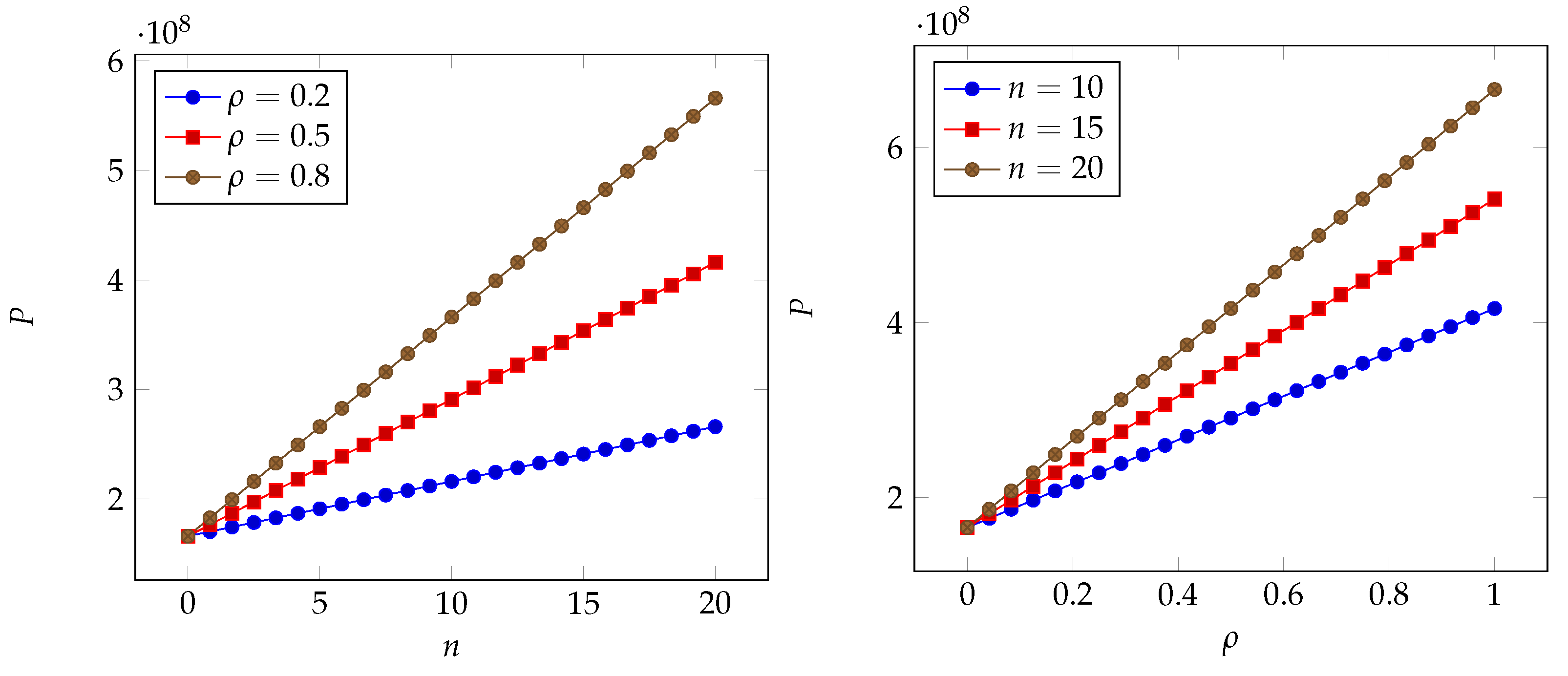
In the following, we report the premium obtained for all these models and show the impact of the number of branches and the correlation coefficient. For each mode, we first propose a bidimensional plot that shows the overall dependence on both parameters, and then show some cuts, where we set one parameter and vary the other.
The pictures pertaining to the scenario proposed by Edwards et al. (2016) are shown in Figure 3 and Figure 4; those for the scenario proposed by Mastroeni et al. (2019) are shown in Figure 5 and Figure 6; those for the scenario proposed by Lin et al. (2018) are shown in Figure 7 and Figure 8; and finally those for the scenario proposed by Wheatley et al. (2016) are shown in Figure 9 and Figure 10.
In all pictures, we can see that a quasi-linear relationship occurs for both parameters. Each parameter works as a booster for the impact of the other. The range due to the proportional term with respect to the baseline case (i.e., no correlation and no branches) is, however, different in each of the scenarios. We observe a very small range (less than 1%) in the scenario considered by Lin et al. (2018), while it approaches close to 50% in the scenarios considered by Edwards et al. (2016) and Mastroeni et al. (2019). It may exceed 100% for the scenario adopted by Wheatley et al. (2016).
7. Conclusions
We have proposed a formula for the insurance premium in the case of correlated risks considering a company with multiple sites (or a network of interconnected companies). The formula is easy to apply and calls for a simple characterization of the correlated risks, requiring just the first two moments (mean and variance) and the correlation coefficient and representing a significant advantage over more complex characterization approaches. We have also shown the resulting premium under several scenarios embodying different probability models for incident frequency and associated losses. The results show that the premium exhibits a quasi-linear relationship with both the number of branches and the risk correlation coefficient among the branches. Thus, each of the two determinants acts as a booster for the impact of the other. The impact of the probability models underlying the risk scenarios is visible through the resulting range of the premium. A comparison with the baseline case (no correlation and no branches) shows that the impact of correlation and the number of branches varies from a few to several hundred percentage points.
As a future research stream, we envisage considering the impact of the incorrect estimation of the breach frequency and associated losses, as well as the role of moral hazard due to the insured not taking suitable countermeasures against cyber risks or not disclosing correct information about its self-protection status.
Author Contributions
Authors contributed equally: methodology, L.M., A.M. and M.N.; writing L.M., A.M. and M.N.; formal analysis L.M., A.M. and M.N.; conceptualization L.M., A.M. and M.N. All authors have read and agreed to the published version of the manuscript.
Funding
This research received no external funding.
Data Availability Statement
Not applicable.
Conflicts of Interest
The authors declare no conflict of interest.
References
- Albadarneh, Aalaa, Israa Albadarneh, and Abdallah Qusef. 2015. Risk management in agile software development: A comparative study. Paper presented at 2015 IEEE Jordan Conference on Applied Electrical Engineering and Computing Technologies (AEECT), Amman, Jordan, November 3–5; pp. 1–6. [Google Scholar]
- Antonio, Yeftanus, Sapto Wahyu Indratno, and Suhadi Wido Saputro. 2021. Pricing of cyber insurance premiums using a markov-based dynamic model with clustering structure. PLoS ONE 16: e0258867. [Google Scholar] [CrossRef]
- Armenia, Stefano, Marco Angelini, Fabio Nonino, Giulia Palombi, and Mario Francesco Schlitzer. 2021. A dynamic simulation approach to support the evaluation of cyber risks and security investments in smes. Decision Support Systems 147: 113580. [Google Scholar] [CrossRef]
- Aven, Terje. 2010. On how to define, understand and describe risk. Reliability Engineering & System Safety 95: 623–31. [Google Scholar]
- Aven, Terje, and Louis Anthony Cox Jr. 2016. National and global risk studies: How can the field of risk analysis contribute? Risk Analysis 36: 186–90. [Google Scholar] [CrossRef] [PubMed]
- Aven, Terje, and Roger Flage. 2020. Foundational challenges for advancing the field and discipline of risk analysis. Risk Analysis 40: 2128–36. [Google Scholar] [CrossRef]
- Babcock, Bruce A., E. Kwan Choi, and Eli Feinerman. 1993. Risk and probability premiums for cara utility functions. Journal of Agricultural and Resource Economics 18: 17–24. [Google Scholar]
- Bandyopadhyay, Tridib, Varghese Jacob, and Srinivasan Raghunathan. 2010. Information security in networked supply chains: Impact of network vulnerability and supply chain integration on incentives to invest. Information Technology and Management 11: 7–23. [Google Scholar] [CrossRef]
- Bandyopadhyay, Tridib, Vijay S. Mookerjee, and Ram C. Rao. 2009. Why it managers do not go for cyber-insurance products. Communications of the ACM 52: 68–73. [Google Scholar] [CrossRef]
- Böhme, Rainer, and Galina Schwartz. 2010. Modeling cyber-insurance: Towards a unifying framework. Paper presented at Workshop on the Economics of Information Security: WEIS, Cambridge, MA, USA, June 7–8. [Google Scholar]
- Böhme, Rainer, and Gaurav Kataria. 2006. Models and measures for correlation in cyber-insurance. Paper presented at Workshop on the Economics of Information Security: WEIS, Cambridge, UK, June 28–30; Volume 2, p. 3. [Google Scholar]
- Böhme, Rainer, Stefan Laube, and Markus Riek. 2019. A fundamental approach to cyber risk analysis. Variance 12: 161–85. [Google Scholar]
- Broner, Fernando, and Jaume Ventura. 2011. Globalization and risk sharing. The Review of Economic Studies 78: 49–82. [Google Scholar] [CrossRef]
- Brunello, Giorgio. 2002. Absolute risk aversion and the returns to education. Economics of Education Review 21: 635–40. [Google Scholar] [CrossRef]
- Bürger, Olga, Björn Häckel, Philip Karnebogen, and Jannick Töppel. 2019. Estimating the impact of it security incidents in digitized production environments. Decision Support Systems 127: 113144. [Google Scholar] [CrossRef]
- Covello, Vincent T., and Jeryl Mumpower. 1985. Risk analysis and risk management: An historical perspective. Risk Analysis 5: 103–20. [Google Scholar] [CrossRef]
- Da, Gaofeng, Maochao Xu, and Peng Zhao. 2021. Multivariate dependence among cyber risks based on l-hop propagation. Insurance: Mathematics and Economics 101: 525–46. [Google Scholar] [CrossRef]
- David, Mihaela. 2015. Auto insurance premium calculation using generalized linear models. Procedia Economics and Finance 20: 147–56. [Google Scholar] [CrossRef]
- Dhaene, Jan, Michel Denuit, Marc J. Goovaerts, Rob Kaas, and David Vyncke. 2002. The concept of comonotonicity in actuarial science and finance: Theory. Insurance: Mathematics and Economics 31: 3–33. [Google Scholar] [CrossRef]
- Dou, Wanchun, Wenda Tang, Xiaotong Wu, Lianyong Qi, Xiaolong Xu, Xuyun Zhang, and Chunhua Hu. 2020. An insurance theory based optimal cyber-insurance contract against moral hazard. Information Sciences 527: 576–89. [Google Scholar] [CrossRef]
- Edwards, Benjamin, Steven Hofmeyr, and Stephanie Forrest. 2016. Hype and heavy tails: A closer look at data breaches. Journal of Cybersecurity 2: 3–14. [Google Scholar] [CrossRef]
- Eeckhoudt, Louis, Christian Gollier, and Harris Schlesinger. 2011. Economic and Financial Decisions under Risk. Princeton: Princeton University Press. [Google Scholar]
- Eling, Martin. 2020. Cyber risk research in business and actuarial science. European Actuarial Journal 10: 303–33. [Google Scholar] [CrossRef]
- Erb, Claude B., Campbell R. Harvey, and Tadas E. Viskanta. 1996. Political risk, economic risk, and financial risk. Financial Analysts Journal 52: 29–46. [Google Scholar] [CrossRef]
- Fahrenwaldt, Matthias A., Stefan Weber, and Kerstin Weske. 2018. Pricing of cyber insurance contracts in a network model. ASTIN Bulletin: The Journal of the IAA 48: 1175–218. [Google Scholar] [CrossRef]
- Fielder, Andrew, Emmanouil Panaousis, Pasquale Malacaria, Chris Hankin, and Fabrizio Smeraldi. 2016. Decision support approaches for cyber security investment. Decision Support Systems 86: 13–23. [Google Scholar] [CrossRef]
- Florackis, Chris, Christodoulos Louca, Roni Michaely, and Michael Weber. 2023. Cybersecurity risk. The Review of Financial Studies 36: 351–407. [Google Scholar] [CrossRef]
- Frigo, Mark L., and Richard J. Anderson. 2011. What is strategic risk management? Strategic Finance 92: 21. [Google Scholar]
- Herath, Hemantha, and Tejaswini Herath. 2011. Copula-based actuarial model for pricing cyber-insurance policies. Insurance Markets and Companies: Analyses and Actuarial Computations 2: 7–20. [Google Scholar]
- Hillairet, Caroline, Olivier Lopez, Louise d’Oultremont, and Brieuc Spoorenberg. 2022. Cyber-contagion model with network structure applied to insurance. Insurance: Mathematics and Economics 107: 88–101. [Google Scholar] [CrossRef]
- Hillson, David, and Ruth Murray-Webster. 2017. Understanding and Managing Risk Attitude. London: Routledge. [Google Scholar]
- Hoang, Dinh Thai, Ping Wang, Dusit Niyato, and Ekram Hossain. 2017. Charging and discharging of plug-in electric vehicles (pevs) in vehicle-to-grid (v2g) systems: A cyber insurance-based model. IEEE Access 5: 732–54. [Google Scholar] [CrossRef]
- Johnson, Benjamin, Aron Laszka, and Jens Grossklags. 2014. How many down? toward understanding systematic risk in networks. Paper presented at 9th ACM Symposium on Information, Computer and Communications Security, Kyoto, Japan, June 4–6; pp. 495–500. [Google Scholar]
- Kaas, Rob, Marc Goovaerts, Jan Dhaene, and Michel Denuit. 2008. Modern Actuarial Risk Theory: Using R. Berlin/Heidelberg: Springer Science & Business Media, Volume 128. [Google Scholar]
- Kaplan, Stan. 1991. Risk assessment and risk management-basic concepts and. In Risk Management: Expanding Horizons in Nuclear Power and Other Industries. Boca Raton: CRC Press, p. 11. [Google Scholar]
- Kaplan, Stanley, and B. John Garrick. 1981. On the quantitative definition of risk. Risk Analysis 1: 11–27. [Google Scholar] [CrossRef]
- Khalili, Mohammad Mahdi, Mingyan Liu, and Sasha Romanosky. 2019. Embracing and controlling risk dependency in cyber-insurance policy underwriting. Journal of Cybersecurity 5: tyz010. [Google Scholar] [CrossRef]
- Khalili, Mohammad Mahdi, Parinaz Naghizadeh, and Mingyan Liu. 2018. Designing cyber insurance policies: The role of pre-screening and security interdependence. IEEE Transactions on Information Forensics and Security 13: 2226–39. [Google Scholar] [CrossRef]
- Kröger, Wolfgang. 2008. Critical infrastructures at risk: A need for a new conceptual approach and extended analytical tools. Reliability Engineering & System Safety 93: 1781–87. [Google Scholar]
- Kunreuther, Howard, and Geoffrey Heal. 2003. Interdependent security. Journal of Risk and Uncertainty 26: 231–49. [Google Scholar] [CrossRef]
- Laeven, Roger J. A., and Marc J. Goovaerts. 2008. Premium calculation and insurance pricing. Encyclopedia of Quantitative Risk Analysis and Assessment 3: 1302–14. [Google Scholar]
- Landsman, Zinoviy, and Michael Sherris. 2001. Risk measures and insurance premium principles. Insurance: Mathematics and Economics 29: 103–15. [Google Scholar] [CrossRef]
- Lau, Pikkin, Lingfeng Wang, Zhaoxi Liu, Wei Wei, and Chee-Wooi Ten. 2021. A coalitional cyber-insurance design considering power system reliability and cyber vulnerability. IEEE Transactions on Power Systems 36: 5512–24. [Google Scholar] [CrossRef]
- Lau, Pikkin, Wei Wei, Lingfeng Wang, Zhaoxi Liu, and Chee-Wooi Ten. 2020. A cybersecurity insurance model for power system reliability considering optimal defense resource allocation. IEEE Transactions on Smart Grid 11: 4403–14. [Google Scholar] [CrossRef]
- Lima Ramos, Pedro. 2017. Premium calculation in insurance activity. Journal of Statistics and Management Systems 20: 39–65. [Google Scholar] [CrossRef]
- Lin, Zhaoxin, Travis Sapp, Rahul Parsa, Jackie Rees Ulmer, and Chengxin Cao. 2018. Pricing cyber security insurance. Journal of Mathematical Finance 12: 46–70. [Google Scholar] [CrossRef]
- Liu, Zhaoxi, Wei Wei, Lingfeng Wang, Chee-Wooi Ten, and Yeonwoo Rho. 2020. An actuarial framework for power system reliability considering cybersecurity threats. IEEE Transactions on Power Systems 36: 851–64. [Google Scholar] [CrossRef]
- Lowrance, William W. 1976. Of Acceptable Risk: Science and the Determination of Safety. Los Altos: William Kaufmann Inc., p. 192. [Google Scholar] [CrossRef]
- Maglaras, Leandros A., Ki-Hyung Kim, Helge Janicke, Mohamed Amine Ferrag, Stylianos Rallis, Pavlina Fragkou, Athanasios Maglaras, and Tiago J Cruz. 2018. Cyber security of critical infrastructures. ICT Express 4: 42–45. [Google Scholar] [CrossRef]
- Marotta, Angelica, Fabio Martinelli, Stefano Nanni, Albina Orlando, and Artsiom Yautsiukhin. 2017. Cyber-insurance survey. Computer Science Review 24: 35–61. [Google Scholar] [CrossRef]
- Martinelli, Fabio, Albina Orlando, Ganbayar Uuganbayar, and Artsiom Yautsiukhin. 2018. Preventing the drop in security investments for non-competitive cyber-insurance market. In Risks and Security of Internet and Systems: Proceedings of the 12th International Conference, CRiSIS 2017, Dinard, France, 19–21 September 2017. Revised Selected Papers 12. Cham: Springer, pp. 159–174. [Google Scholar]
- Mastroeni, Loretta, Alessandro Mazzoccoli, and Maurizio Naldi. 2019. Service level agreement violations in cloud storage: Insurance and compensation sustainability. Future Internet 11: 142. [Google Scholar] [CrossRef]
- Mazzoccoli, Alessandro, and Maurizio Naldi. 2020a. The expected utility insurance premium principle with fourth-order statistics: Does it make a difference? Algorithms 13: 116. [Google Scholar] [CrossRef]
- Mazzoccoli, Alessandro, and Maurizio Naldi. 2020b. Robustness of optimal investment decisions in mixed insurance/investment cyber risk management. Risk Analysis 40: 550–64. [Google Scholar] [CrossRef]
- Mazzoccoli, Alessandro, and Maurizio Naldi. 2021. Optimal investment in cyber-security under cyber insurance for a multi-branch firm. Risks 9: 24. [Google Scholar]
- Mazzoccoli, Alessandro, and Maurizio Naldi. 2022. Optimizing cybersecurity investments over time. Algorithms 15: 211. [Google Scholar] [CrossRef]
- Nagurney, Anna, and Shivani Shukla. 2017. Multifirm models of cybersecurity investment competition vs. cooperation and network vulnerability. European Journal of Operational Research 260: 588–600. [Google Scholar] [CrossRef]
- Naldi, Maurizio, and Alessandro Mazzoccoli. 2018. Computation of the insurance premium for cloud services based on fourth-order statistics. International Journal of Simulation: Systems, Science and Technology 19: 1–6. [Google Scholar] [CrossRef]
- Olivieri, Annamaria, and Ermanno Pitacco. 2015. Introduction to Insurance Mathematics: Technical and Financial Features of Risk Transfers. Berlin/Heidelberg: Springer. [Google Scholar]
- Öğüt, Hulisi, Srinivasan Raghunathan, and Nirup Menon. 2011. Cyber security risk management: Public policy implications of correlated risk, imperfect ability to prove loss, and observability of self-protection. Risk Analysis: An International Journal 31: 497–512. [Google Scholar] [CrossRef] [PubMed]
- Paté-Cornell, M-Elisabeth, Marshall Kuypers, Matthew Smith, and Philip Keller. 2018. Cyber risk management for critical infrastructure: A risk analysis model and three case studies. Risk Analysis 38: 226–41. [Google Scholar] [CrossRef] [PubMed]
- Peng, Chen, Maochao Xu, Shouhuai Xu, and Taizhong Hu. 2018. Modeling multivariate cybersecurity risks. Journal of Applied Statistics 45: 2718–40. [Google Scholar] [CrossRef]
- Peterson, Kevin E. 2020. What is risk management? In The Professional Protection Officer. Amsterdam: Elsevier, pp. 367–72. [Google Scholar]
- Power, Michael. 2005. The invention of operational risk. Review of International Political Economy 12: 577–99. [Google Scholar] [CrossRef]
- Refsdal, Atle, Bjørnar Solhaug, and Ketil Stølen. 2015. Cyber-risk management. In Cyber-Risk Management. Berlin/Heidelberg: Springer, pp. 33–47. [Google Scholar]
- Straub, Erwin, and Swiss Association of Actuaries (Zürich). 1988. Non-Life Insurance Mathematics. Number 517/S91n. Berlin/Heidelberg: Springer. [Google Scholar]
- Su, Karen C., Chung-Bow Lee, Shu-Hui Lin, I-Chien Liu, and Hong-Chi Chen. 2021. Pricing cyber risk: The copula-based approach. In Advances in Pacific Basin Business, Economics and Finance. Bingley: Emerald Publishing Limited. [Google Scholar]
- Weber, Elke U. 2010. Risk attitude and preference. Wiley Interdisciplinary Reviews: Cognitive Science 1: 79–88. [Google Scholar] [CrossRef]
- Wheatley, Spencer, Thomas Maillart, and Didier Sornette. 2016. The extreme risk of personal data breaches and the erosion of privacy. The European Physical Journal B 89: 1–12. [Google Scholar] [CrossRef]
- Xie, Danyang. 2000. Power risk aversion utility functions. Annals of Economics and Finance 1: 265–82. [Google Scholar]
- Xu, Lu, Yanhui Li, and Jing Fu. 2019. Cybersecurity investment allocation for a multi-branch firm: Modeling and optimization. Mathematics 7: 587. [Google Scholar] [CrossRef]
- Yang, Zhiyuan, Yun Liu, Meghan Campbell, Chee-Wooi Ten, Yeonwoo Rho, Lingfeng Wang, and Wei Wei. 2020. Premium calculation for insurance businesses based on cyber risks in ip-based power substations. IEEE Access 8: 78890–900. [Google Scholar] [CrossRef]
- Young, Derek, Juan Lopez Jr., Mason Rice, Benjamin Ramsey, and Robert McTasney. 2016. A framework for incorporating insurance in critical infrastructure cyber risk strategies. International Journal of Critical Infrastructure Protection 14: 43–57. [Google Scholar] [CrossRef]
- Zhang, Yunfan, Lingfeng Wang, Zhaoxi Liu, and Wei Wei. 2020. A cyber-insurance scheme for water distribution systems considering malicious cyberattacks. IEEE Transactions on Information Forensics and Security 16: 1855–67. [Google Scholar] [CrossRef]
- Zio, Enrico. 2007. An Introduction to the Basics of Reliability and Risk Analysis. Singapore: World Scientific, Volume 13. [Google Scholar]
Figure 1.
An example of a bidimensional exponential utility function ( and ).

Figure 2.
Ratio between the risk aversion coefficients and .
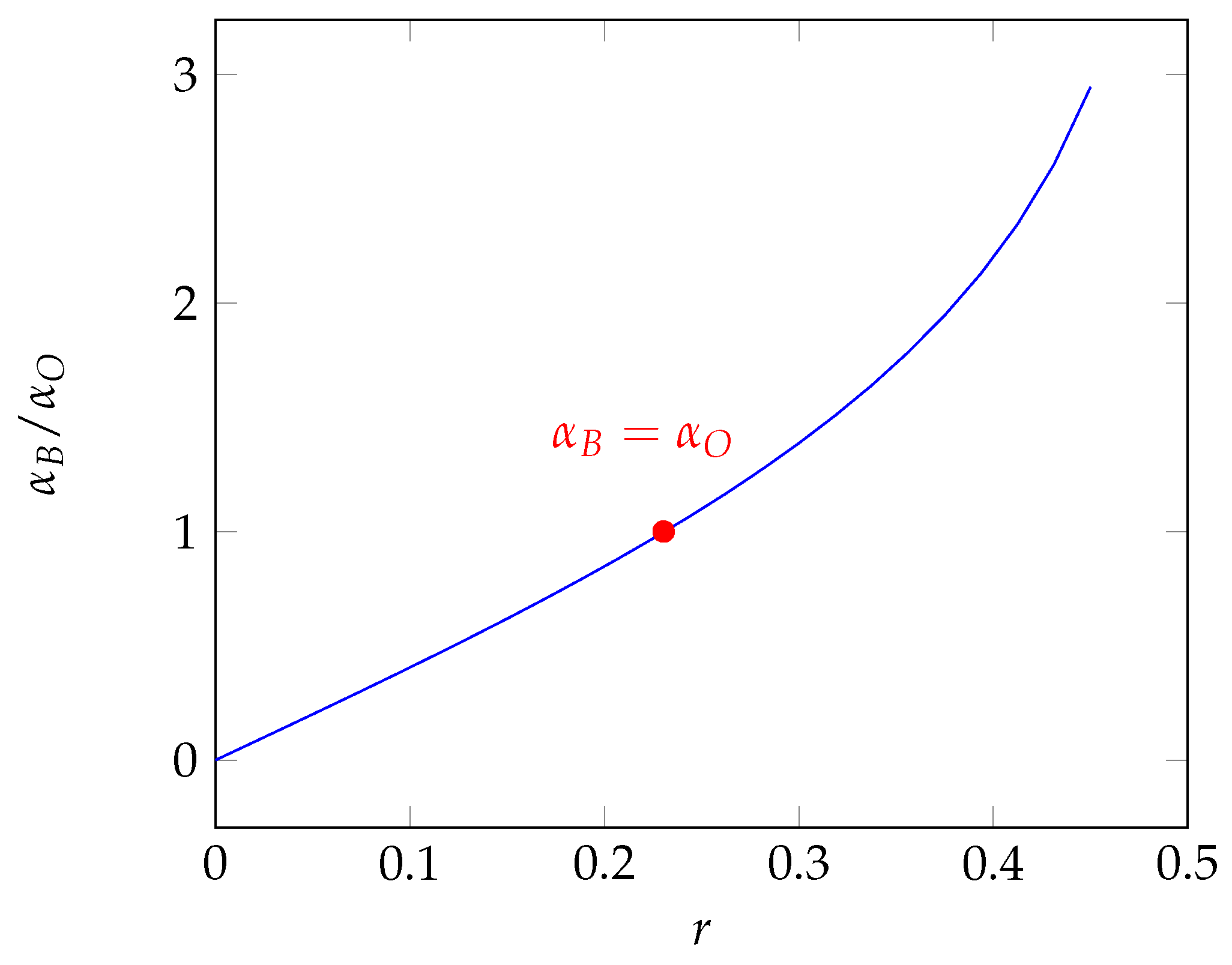
Figure 3.
Impact of the number of branches n and the correlation coefficient on the insurance premium P (scenario as proposed by Edwards et al. (2016)).
Figure 3.
Impact of the number of branches n and the correlation coefficient on the insurance premium P (scenario as proposed by Edwards et al. (2016)).
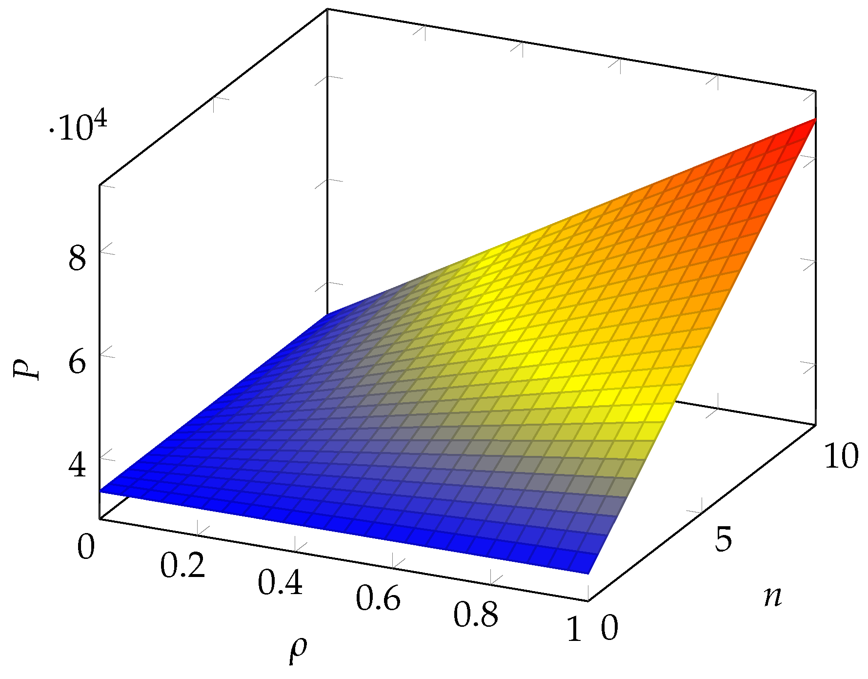
Figure 4.
Left: impact of the number of branches n on the insurance premium; right: impact of the correlation coefficient on the insurance premium (scenario as proposed by Edwards et al. (2016)).
Figure 4.
Left: impact of the number of branches n on the insurance premium; right: impact of the correlation coefficient on the insurance premium (scenario as proposed by Edwards et al. (2016)).

Figure 5.
Impact of the number of branches n and the correlation coefficient on the insurance premium P (scenario as proposed by Mastroeni et al. (2019)).
Figure 5.
Impact of the number of branches n and the correlation coefficient on the insurance premium P (scenario as proposed by Mastroeni et al. (2019)).

Figure 6.
Left: impact of the number of branches n on the insurance premium; right: impact of the correlation coefficient on the insurance premium (scenario as proposed by Mastroeni et al. (2019)).
Figure 6.
Left: impact of the number of branches n on the insurance premium; right: impact of the correlation coefficient on the insurance premium (scenario as proposed by Mastroeni et al. (2019)).

Figure 7.
Impact of the number of branches n and the correlation coefficient on the insurance premium P (scenario as proposed by Lin et al. (2018)).
Figure 7.
Impact of the number of branches n and the correlation coefficient on the insurance premium P (scenario as proposed by Lin et al. (2018)).

Figure 8.
Left: Impact of the number of branches n on the insurance premium; right: Impact of the correlation coefficient on the insurance premium (scenario as proposed by Lin et al. (2018)).
Figure 8.
Left: Impact of the number of branches n on the insurance premium; right: Impact of the correlation coefficient on the insurance premium (scenario as proposed by Lin et al. (2018)).
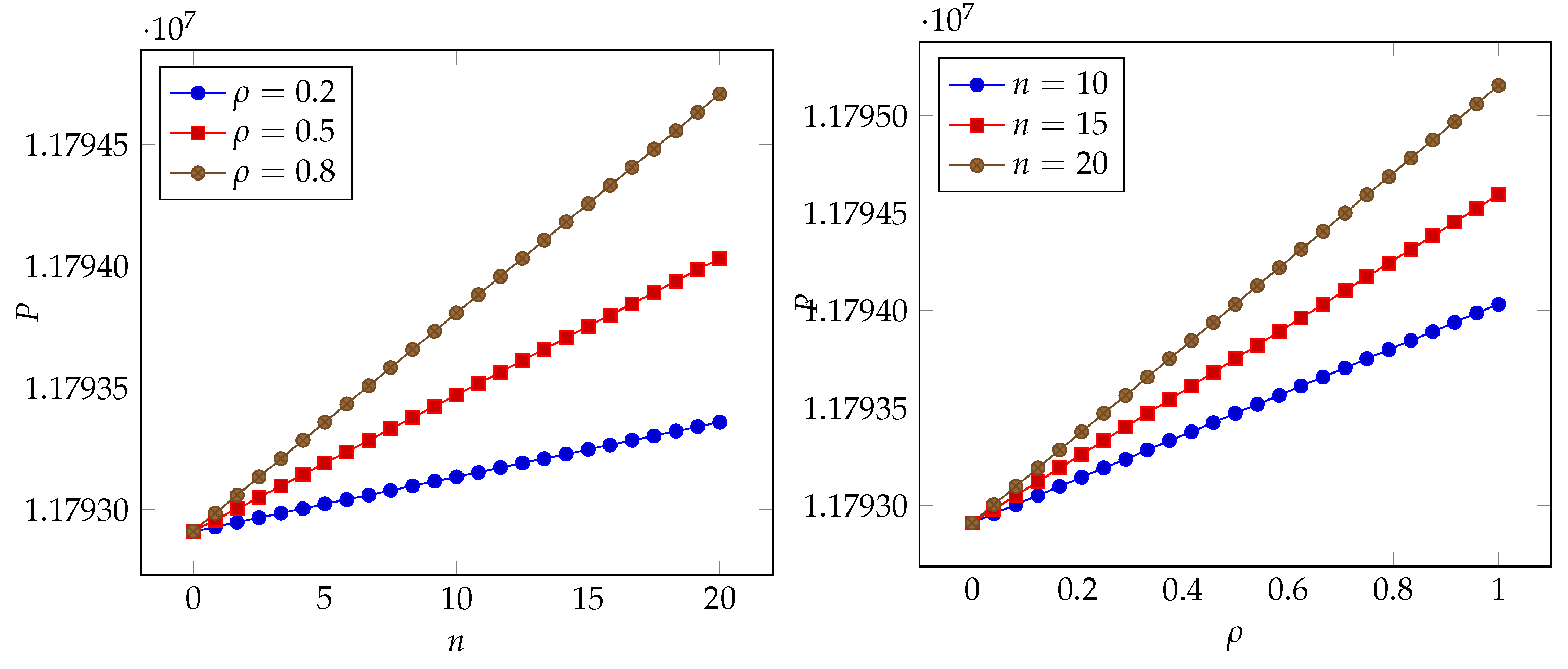
Figure 9.
Impact of the number of branches n and the correlation coefficient on the insurance premium P (scenario as proposed by Wheatley et al. (2016)).
Figure 9.
Impact of the number of branches n and the correlation coefficient on the insurance premium P (scenario as proposed by Wheatley et al. (2016)).
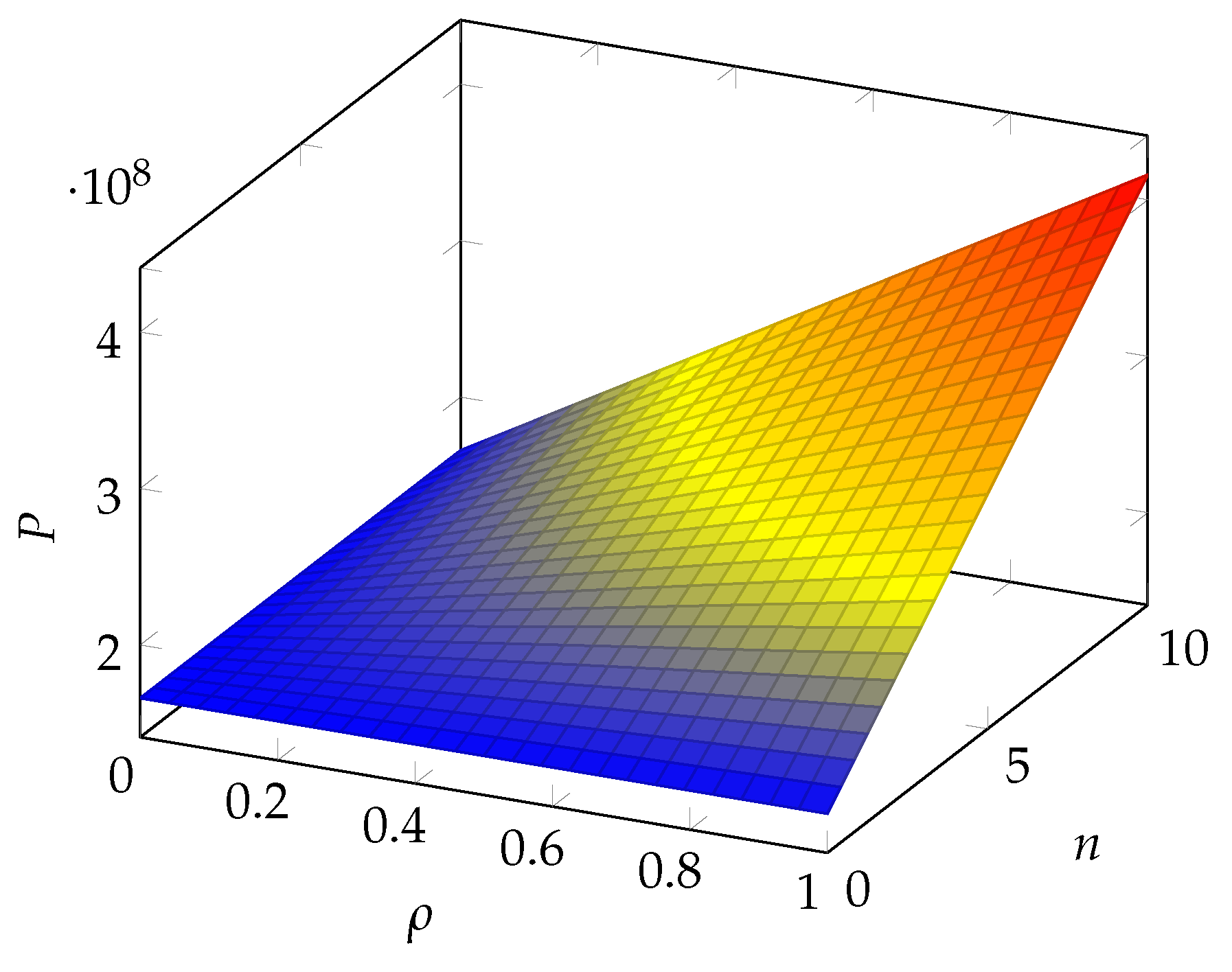
Figure 10.
Left: impact of the number of branches n on the insurance premium; right: impact of the correlation coefficient on the insurance premium (scenario as proposed by Wheatley et al. (2016)).
Figure 10.
Left: impact of the number of branches n on the insurance premium; right: impact of the correlation coefficient on the insurance premium (scenario as proposed by Wheatley et al. (2016)).

Table 1.
Glossary.
| Parameter | Meaning |
|---|---|
| u | Utility function |
| w | Firm asset |
| X | Monetary loss variable |
| P | Insurance premium |
| Risk aversion coefficient | |
| r | Risk premium |
| Correlation coefficient |
Table 2.
Frequency and average annual loss in the scenarios considered.
| Scenarios | Frequency | Avg Loss (USD) |
|---|---|---|
| Edwards et al. (2016) | 0.008 | 2.82 |
| Mastroeni et al. (2019) | 0.036 | 8.6 |
| Lin et al. (2018) | 0.032 | 1.2 |
| Wheatley et al. (2016) | 0.38 | 1.4 |
Disclaimer/Publisher’s Note: The statements, opinions and data contained in all publications are solely those of the individual author(s) and contributor(s) and not of MDPI and/or the editor(s). MDPI and/or the editor(s) disclaim responsibility for any injury to people or property resulting from any ideas, methods, instructions or products referred to in the content. |
© 2023 by the authors. Licensee MDPI, Basel, Switzerland. This article is an open access article distributed under the terms and conditions of the Creative Commons Attribution (CC BY) license (https://creativecommons.org/licenses/by/4.0/).
Share and Cite
MDPI and ACS Style
Mastroeni, L.; Mazzoccoli, A.; Naldi, M. Cyber Insurance Premium Setting for Multi-Site Companies under Risk Correlation. Risks 2023, 11, 167. https://doi.org/10.3390/risks11100167
AMA Style
Mastroeni L, Mazzoccoli A, Naldi M. Cyber Insurance Premium Setting for Multi-Site Companies under Risk Correlation. Risks. 2023; 11(10):167. https://doi.org/10.3390/risks11100167
Chicago/Turabian StyleMastroeni, Loretta, Alessandro Mazzoccoli, and Maurizio Naldi. 2023. "Cyber Insurance Premium Setting for Multi-Site Companies under Risk Correlation" Risks 11, no. 10: 167. https://doi.org/10.3390/risks11100167
Note that from the first issue of 2016, this journal uses article numbers instead of page numbers. See further details here.