Modeling Cycle Dependence in Credit Insurance

Abstract

Business and credit cycles have an impact on credit insurance, as they do on other businesses. Nevertheless, in credit insurance, the impact of the systemic risk is even more important and can lead to major losses during a crisis. Because of this, the insurer surveils and manages policies almost continuously. The management actions it takes limit the consequences of a downturning cycle. However, the traditional modeling of economic capital does not take into account this important feature of credit insurance. This paper proposes a model aiming to estimate future losses of a credit insurance portfolio, while taking into account the insurer’s management actions. The model considers the capacity of the credit insurer to take on less risk in the case of a cycle downturn, but also the inverse, in the case of a cycle upturn; so, losses are predicted with a more dynamic perspective. According to our results, the economic capital is over-estimated when not considering the management actions of the insurer.

1. Introduction

Credit insurance is concerned with business and credit cycle fluctuations, but in an unusual way. Indeed, it is extremely impacted by the defaults at the beginning of a crisis, but afterwards, the influence of the cycle downturn lowers the impact in a relatively short amount of time.

Commercial businesses need a credit insurer if they think their clients will not be able to pay their invoices on time or risk becoming insolvent shortly. Therefore, they obtain an insurance policy that guarantees them that a part of or the whole invoice amount will be reimbursed by the insurer in the case that the client could not pay. Every company may obtain an insurance policy to insure against the default payment of its clients, so small businesses and very big companies are insured.

Thus, the credit insurer takes on the risk of insolvency or protracted default.1 This makes the credit insurer very sensitive to credit and, eventually, business cycles.

While the type of risk the insurer bears is still a credit risk, it is quite different from the credit risk of financial markets. First, because the source of risk is very diversified, defaulting firms can come from very different sectors: they can be small around-the-corner businesses or big multinational corporations. Second, the risk is not quoted in a market; there is no bid or sale. Therefore, the credit insurer should manage its portfolio, along with the cycles and its risk aversion, and thus, management actions will not be the same during this period. We will try to take this into account.

Many papers aim to find out whether business and credit cycles coincide, and it seems there is no final answer to this question (see, for example, [1,2] and the references therein). Both cycles seem to follow some macro-economic variables, and GDP variations seem to explain, at least partly, credit cycle movements. Anyway, the difference between these two cycles will not be important in what follows. We can work with either of them, as long as we distinguish upturns from downturns; that in downturn periods there are (significantly) more defaults than in upturn periods and that the hypothesis that the cycles are a Markov process are realistic. For us, the important issue will be being able to distinguish the point at which the number of defaults changes significantly, i.e., at which the default regime switches.

When the cycle goes down, the number of insolvent firms or those not being able to pay their invoices increases dramatically. Hence, the insurer should reimburse huge amounts of money, and it risks becoming insolvent itself. This would probably be the case if credit insurers could not limit their losses. They can do this by diminishing their exposure towards firms (clients of the insured business) whose creditworthiness is decreasing. In this case, the insurer warns the insured firm , whose granted amount is decreased. Its client may not be solvent anymore, and it should itself reduce the amount of commercial exchanges with the client. On the other hand, when the insurer thinks that economic conditions are more favorable, it takes on more risk and increases the guarantees. See [3] for an introduction to risk mitigation in credit insurance.

The large number of firms defaulting at the same time at the beginning of a crisis impacts the credit insurer quite considerably (if the insurer has not correctly predicted the starting point of the crisis). However, once the number of defaults increases and the consequences of the crisis are observed, the credit insurer can lower its exposures towards riskier firms; there is a trade-off between the immediate loss of money and subsequent credibility loss (which would mean a loss of future wealth) and the diminishing of its losses. To resume, the insurer has the power to increase or decrease the risk it is bearing, which is more difficult for banks, for example.

For all these reasons, it is important for a credit insurer to predict the state of the economy and for the actuarial teams to compute a risk capital, which depends on the state of the economy. The insurer computes its economic capital for a one-year period. In the current modeling, its capability to take actions on the exposures and portfolio is ignored, and this actually leads to an overestimation of its reserves. The reason for this is that the consequences of lowering its exposures in hard times are bigger and faster than those of increasing the risk appetite in prosperous periods.

Our paper presents a way to adjust to cycles and to introduce lowering or increasing exposures. In the first section, we will present the reference model, where all parameters are fixed during the period. In the second section, we will introduce a two-period modeling, which allows one to adjust to the cycle. In the last section, we apply the model to a credit insurance portfolio and compare the values of economic capital under the two models.

2. Reference Single-Period Modeling

The model we will introduce in this section is the cornerstone of the two-period model we propose. Let us start by describing this model, so that the new steps we want to introduce and their usefulness may be clearer later on.

2.1. Default Modeling

Defaults are currently modeled with a multi-factor Merton model. The model is Merton-like (see [4,5,6,7]), since one client, which we will henceforth call the buyer, will default if a latent value, called the ability to pay and notated as Z, falls below a certain threshold, d. In the true Merton model, the latent value is the value of the assets of the firm, and the firm defaults if its assets value fall below the amount of its liabilities. The probability of default for buyer n is then:

$$p_n=\mathbb{P}\left(Z_n\le d_n\right)$$

The parameter estimated here is not the default threshold, because we are working with a latent variable, but rather, the default probabilities, $p_n$. In our case, we will assume that they are given and are exogenous to our main concern.

The default modeling is a multi-factor one, because the latent variable, $Z_n$, is modeled as the sum of systemic risk and buyer individual risk. See [8,9,10,11,12] for further information on one-factor and multi-factor models and the associated copulae.

In our case, we have:

$$Z_n={\varrho }_n{}^t{w}_{n}R+\sqrt{1-{\varrho }_n^2}{\epsilon }_n$$

where:

• R is the systemic risk vector following a multivariate Gaussian distribution, $N\left(0,\Sigma \right)$, with Σ the covariance matrix. In our case, it is a $(105,105)$ type of matrix;
• ${\epsilon }_n$ is the idiosyncratic (individual) risk of buyer n and follows a standard Gaussian distribution, $N\left(0,1\right)$;
• ${\epsilon }_n$ and R are independent;
• $w_n$ is the vector of weights of buyer n for risk factors in R;
• ${\varrho }_n$ describes the correlation of buyer n to systemic risk (economy); the bigger it is, the higher the correlation to systemic risk, thus the higher the correlation between firms.

In the multi-factor model, the parameters one needs to estimate are the covariance matrix, Σ, ${\varrho }_n$, and the weights, $w_n$. In practice, the estimation of Σ and ${\varrho }_n$ seems to be the hardest part, but it will not be the object of our paper.

We should also notice that since it is easier to manipulate standard Gaussian variables, and $Z_n$ with the above definition is not a standard one, we will use instead the following definition of Z:

$$Z_n={\varrho }_n{\displaystyle \frac{{}^t{w}_{n}R}{\parallel {}^t{w}_{n}M\parallel }}+\sqrt{1-{\varrho }_n^2}{\epsilon }_n$$

where M is such that Σ = ${}^{t}MM$ (after the Cholesky decomposition of Σ).

2.2. Loss Modeling

A defaulting buyer will produce a loss. This loss will be equal to the insured amount, which is defined as the minimum value among the invoice amount and the exposure the insurer has on the buyer.2

$$\text{Loss}{}_n=min\left(\text{Invoice}{\text{Amount}}_n;{\text{Exposure}}_n\right)$$

Since the insured amount is not known until the default occurs, it is modeled through UGDs (Usage Given Default), defined with the following formula:

$$\text{UGD}={\displaystyle \frac{\mathit{Insured}{\mathit{amount}}_n}{{\mathit{Exposure}}_n}}$$

$\text{UGD}{}_n$ is another parameter the insurer should model and estimate. Given $\text{UGD}$, the insurer estimates the loss from buyer n to be equal to:

$$\text{Loss}{}_n={\text{UGD}}_n\times {\text{Exposure}}_n$$

in case buyer n defaults.3

3. A New Modeling Approach-Taking into Account the Actions of Management

The current modeling is single period, which means that the whole parameters as well as the considered variables are defined over one period. The ability to pay is the one-period ability to pay. If there is a default, there is one default in the period. Since we do not know exactly when it occurs, we assume that all defaults occur at the end of the period. In practice, the period we work on is a year, since reserves are computed on a one-year basis.

We want to introduce into the modeling the possibility for the insurer to manage exposures during the year. Indeed, it can lower exposures for buyers whose creditworthiness decreases and even cancel them, and this has an impact on its reserves.4

Therefore, thanks to this type of management, the reserves of the credit insurer should be lower than those estimated with the one-period model, and we want to take this into consideration.

For this, we will introduce a half-period step into the model, which gives us a two-period model. This two-period model can easily be transposed into a multi-period model.

Nevertheless, in credit insurance, working on a semester basis is coherent and sufficient, since it corresponds to an average reaction time. This means that six months after the beginning of a crisis, the big management actions have already taken place, and so, exposures on very risky firms have been cut or canceled. Therefore, if they are to change substantially, the portfolio features are to change every six months. Thus, the reserves estimated with this model should be more realistic.

3.1. Two-Period Modeling

We will describe here the general idea of the model and deduce afterwards the parameters to be estimated.

The idea here is to divide the single period into two sub-periods.

3.1.1. First Period

The parameters are predicted for the first period. The default probabilities are the parameters we are more interested in, for now. They withhold information about the phase of the cycle in which we are during the period.

At the end of the period, we compute the number of insolvencies, and given a criterion applied to this number, we determine if it is more probable for the first period to be in a high or a low cycle phase. We will give more details about this criterion in the section below.

We then compute the losses related to insolvency defaults and protracted defaults.

The creditworthiness of buyers may change at the end of the period, and their grades may change, consequently; whereas, in the one-period model, buyers could change the rating class only at the end of the period.

3.1.2. Second Period

At the beginning of the second period, we thus have a new portfolio, since the buyers might have changed their grading class, and some of them have defaulted, so they have exited the portfolio.

The exposures might also have changed from the beginning of the first period if the creditworthiness is lower. In the single-period model, this was not possible.

The cycle phase of the second period may be high or low;5 this depends on the a posteriori phase of the cycle in the first period.

The dependence is modeled by a Markov chain, i.e., the probabilities of transition between high or low cycle phases. Examples in the literature are many: for example [13], where they work with business cycles.

The losses of the second period are then added to those of the first.

3.1.3. Parameters

The parameters we need to estimate for the recession and expansion periods are then the following, for low or high cycle phases:

• grade transition matrices, with insolvency probability defaults in the last column, notated as $P_l$ and $P_h$;
• a vector of protracted default probabilities for each grade, ${\pi }_l$ and ${\pi }_h$;
• a vector with UGDs for each grade, $UG{D}_l$ and $UG{D}_h$;
• a vector (or matrix) of coefficients indicating the variation of exposures, $c_l$ and $c_h$.

The parameters for the first period should be predicted, especially the insolvency default probabilities. The grade transition matrix should be given, too.

The estimation of those parameters will not be the object of this article, but finding consistent estimators for those parameters would be of great interest in a future work. A consistent estimation approach would be a hidden Markov chain (or regime-switching Markov chain; see [13,14,15]). Some other papers that present estimation techniques for conditional (on business, credit cycles or other) factors are [1,16,17,18,19,20].

3.1.4. Mathematical Computation of the Losses

Let N be the total number of buyers in the portfolio.

Let $L_n$ be the exposure of buyer n at the beginning of the period.

Let $G_n$ be the grade of buyer n at the beginning of the period, $G_n\in \left\{1,\dots ,J\right\}$, where J is the number of grading classes.

Losses of the first period. The total loss at the end of the first period will be:

$${\text{Loss}}_1=\sum _{n=1}^N{L}_n\times \text{UGD}\left(G_n\right)\times \left[Z_n\le d\left(G_n\right)\right]$$

where $\left[.\right]$ denotes the Iverson bracket.

Remark 1. 

In the formula, we have UGD_Gn, because the UGDs are estimated by the grades and the probabilities of default, too. Practically, we compute $d\left(G_n\right)$ for each grade as a standard Gaussian quantile $d\left(G_n\right)={\Phi }^{-1}\left(p_{G_n}\right)$, where Φ denotes the cumulative distribution function of a standard normal distribution, as does $Z_n$.

Changes in the portfolio during the first period. Let def be the number of defaults in the first period, $\text{def}={\sum }_{n=1}^N\left[Z_n\le d\left(G_n\right)\right]$. If the default rate ${\displaystyle \frac{\text{def}}{N}}={\sum }_{n=1}^N{\displaystyle \frac{\left[Z_n\le d\left(G_n\right)\right]}{N}}$ satisfies a certain criterion, then we suppose the state of the first period was $E_l$; otherwise, we suppose it was $E_h$. We will develop this in 3.2.

Concerning transitions between grades, the same principles as for defaults apply: default thresholds are computed using the transition matrices, P, and the assumption on Z being a standard Gaussian.

The probability for a buyer, n, to go from $G_n=i$ to $j\in \left\{1,\dots ,J\right\}$ is the following:

$$\mathbb{P}\left(d_{i,j+1}\le Z\le d_{ij}\right)=\Phi \left(d_{ij}\right)-\Phi \left(d_{i,j+1}\right)=p_{ij}$$

with $d_{i,j+1}\le d_{ij}$.

The thresholds, $d_{ij}$, of going from Grade i to Grade j are computed:

$$\begin{array}{c}\hfill \forall j\in \left\{J,\dots ,1\right\},d_{ij}={\Phi }^{-1}\left(\sum _{k=j}^{J-1}{p}_{ik}+p_i\right)\end{array}$$

(1)

where $J=10$ in our case.

At the end of the first period, the structure of the portfolio would have changed: buyers having defaulted have exited the portfolio, and the others may have changed grades, which implies that their characteristics, such as, for example, the default probabilities, change for the second period.

Losses in the second period. The transition matrix on the second period will be given conditionally on the cycle phase in the first period.

$$\begin{array}{c}\hfill P_2=\left\{\begin{array}{cc}{P}_h,\hfill & \mathrm{with} \mathrm{probability}\mathbb{P}\left(E_2=h|E\right)\hfill \\ P_l,\hfill & \mathrm{with} \mathrm{probability}\mathbb{P}\left(E_2=l|E\right)\hfill \end{array}\right.\end{array}$$

The protracted default probabilities will be randomly chosen, conditional on the first period, so that:

$$\begin{array}{c}\hfill {\pi }_2=\left\{\begin{array}{cc}{\pi }_h,\hfill & \mathrm{with} \mathrm{probability}\mathbb{P}\left(E_2=h|E\right)\hfill \\ {\pi }_l,\hfill & \mathrm{with} \mathrm{probability}\mathbb{P}\left(E_2=l|E\right)\hfill \end{array}\right.\end{array}$$

We compute a new default threshold with Formula (1) for high and low cycle phases, and then, we just have to choose between the two.

The losses of the second period are given by the formula:

$${\text{Loss}}_2=\sum _{n=1}^{N-\text{def}}{L}_n^2\times \text{UGD}(E,G_n^2)\times \left[Z_n^2\le d^2\left(G_n^2\right)\right]$$

where $L_n^2$ is the exposure of buyer n at the beginning of the second period. It is estimated to be equal to $c_n\times L_n$, where $c_n$ is a coefficient indicating if the exposure of grade n has fallen or increased.

The estimation of the coefficients, $c_n$, is highly important. They can be estimated using the history of claims declarations and seeing how the exposure of buyers who have defaulted has evolved during the year before the default. We would expect that in high cycles, the exposures go up, and when the cycle is low, the exposures fall. Ideally, we could estimate a matrix, C, of coefficients indicating the evolution of the exposure for buyers going from one grade to another. However, in order to have more observations and a more robust estimation, we choose to give a vector of coefficients, indicating the evolution of exposures of buyers relative to their grade at the beginning of the period.

The total loss of the year would then be $\text{Loss}={\text{Loss}}_1+{\text{Loss}}_2$.

3.2. Hypothesis

If the default rate at the end of the period is “high enough”, namely ${\sum }_{n=1}^N{\displaystyle \frac{\left[Z_n\le d\left(G_n\right)\right]}{N}}>{\text{def}}^{★}$, then $E_l$ is more probable than $E_h$. Otherwise, $E_h$ is more probable than $E_l$.

Proposition 1. 

The default rate for a given R, notated as ${\displaystyle \frac{def}{N}}$, is a good estimator of the mean of conditional probabilities of all buyers in the portfolio $\frac{1}{N}{\sum }_{n=1}^N{p}^{n|R}$.

Proof. 

We will use Kolmogorov’s theorem; see the Appendix.

We may apply Kolmogorov’s theorem to the “sequence” of random variables representing conditional default, i.e., $X_n=\left[Z_n\le d_n|R\right]=\left[{ϵ}_n\le \frac{d_n-{\varrho }_{n}R}{\sqrt{1-{\varrho }_n^2}}|R\right]$ for $n=1,\dots ,N$. Indeed, those variables are independent $\left({ϵ}_n\right)$ for $n=1,\dots ,N$.

We choose $a_n=n$ for $n=1,\dots ,+\infty$.

The first hypothesis is satisfied.

$$\begin{array}{ccc}\hfill \mathbb{E}{\left(\left[Z_n\le d_n|R\right]\right)}^2& =& \mathbb{V}\left(\left[Z_n\le d_n|R\right]\right)+{\left(\mathbb{E}\left(\left[Z_n\le d_n|R\right]\right)\right)}^2\hfill \end{array}$$

(2)

$$\begin{array}{ccc}& =& p^{n|R}(1-p^{n|R})+{\left(p^{n|R}\right)}^2=p^{n|R}<1\hfill \end{array}$$

(3)

The second hypothesis is satisfied, since we have:

$$\begin{array}{c}\hfill \sum _{n=1}^{+\infty }{\displaystyle \frac{\mathbb{V}\left(\left[Z_n\le d_n|R\right]\right)}{n^2}}=\sum _{n=1}^{+\infty }{\displaystyle \frac{p^{n|R}(1-p^{n|R})}{n^2}}<\sum _{n=1}^{+\infty }{\displaystyle \frac{1}{4n^2}}<+\infty \end{array}$$

(4)

So

$${\displaystyle \frac{{\sum }_{n=1}^N\left[Z_n\le d_n|R\right]-\mathbb{E}\left({\sum }_{n=1}^N\left[Z_n\le d_n|R\right]\right)}{N}}⟶0\text{a.s.}$$

Then, using the following:

$$\begin{array}{ccc}\hfill \frac{1}{N}\mathbb{E}\left(\sum _{n=1}^N\left[Z_n\le d_n\right]|R\right)& =& \sum _{n=1}^N\mathbb{P}\left(Z_n\le d_n|R\right)\hfill \end{array}$$

(5)

$$\begin{array}{ccc}& =& \frac{1}{N}\sum _{n=1}^N{p}^{n|R}\hfill \end{array}$$

(6)

$$\begin{array}{c}\hfill \frac{1}{N}\sum _{n=1}^N\left[Z_n\le d_n|R\right]-\frac{1}{N}\sum _{n=1}^N{p}^{n|R}⟶0\text{a.s.}\end{array}$$

(7)

Thus, the observed default rate for a given R is a converging estimator of the conditional expectation of the mean of the Bernoulli random variables representing defaults. This estimator is unbiased and efficient.     ☐

Remark 2. 

The sum of the individual conditional probabilities of defaulting will always be greater in a low rather than in a high cycle.

This is due to the fact that if $p_n^r>p_n^e$, then ${\Phi }^{-1}\left(p_n^r\right)=d_n^r>{\Phi }^{-1}\left(p_n^e\right)=d_n^e$.

Then:

$$\frac{1}{N}\sum _{n=1}^N\mathbb{P}\left({\epsilon }_n\le {\displaystyle \frac{d_n^r-{\varrho }_n{w}_{n}R}{\sqrt{1-{\varrho }^2}}}|R\right)>\frac{1}{N}\sum _{n=1}^N\mathbb{P}\left({\epsilon }_n\le {\displaystyle \frac{d_n^e-{\varrho }_n{w}_{n}R}{\sqrt{1-{\varrho }^2}}}|R\right)$$

Therefore, conditionally on R, the number of defaults will always be greater in a low cycle than in a high cycle. Sometimes, for some R observations, the difference between the two conditional probabilities will not be very high, and other times, the change between the two will be a lot greater. Thus, the R vector implies a certain correlation structure between the buyers, which is always greater in a recession than in an expansion. The following is the plot of approximations of the distribution of defaults, in low (black) and in high (red) cycle phases.

Figure 1. Approximations of default distributions.

Figure 1. Approximations of default distributions.

We can see that the two density functions intersect at a certain point. This means that for this point, $\text{def}★$, the probability of having this number of defaults in a low cycle is the same as the one in a high cycle. For default numbers lower than ${\text{def}}^{★}$, $\text{def}<{\text{def}}^{★}$ , the probability that they are coming from a high cycle phase is greater than the probability that they they come from a low cycle phase; and vice versa for $\text{def}>{\text{def}}^{★}$. We may also compute a posteriori probabilities of being in a high or a low cycle.

The data we enter into the model are made of default probabilities, which contain inherent information on being in a high or low cycle phase. With the previous rule, we “decode” this information. After applying the rule, we will know if these probabilities are more alike those in high or low cycles. In practice, this is deduced from the number of cases, where we “fall” into low cycle phases, notated as $x_l$, and in high cycle phases, $x_h$. If $x_h>x_l$, the probabilities entering the model “describe” an economy state closer to a high cycle phase rather than to a low cycle one.

Remark 3. 

We want to emphasize the fact that the more disjoint the two densities are, the better we can recognize a cycle phase just by computing the number of defaults in it. This is why, if just the business credit cycle phases cannot be distinguished well regarding the number of defaults, relevant macro-variables should be tested.

4. Algorithm and Simulations

There is no closed formula for the loss quantiles, and we should use Monte Carlo simulations to find them. In this section, we describe the algorithm and simulations necessary to have the loss distribution numerically.

We have computed all default thresholds.

$$p{d}_2={\text{pd}}_h\times \mathbb{P}\left(E_2=h|E\right)+{\text{pd}}_l\times \mathbb{P}\left(E_2|E\right)$$

For each simulation $t=\left\{1,\dots ,T\right\}$:

(1)

Simulate $R^t$ following a multivariate Gaussian distribution, $N\left(0,\Sigma \right)$.

(2)

Simulate N independent standard Gaussian variables, ${\epsilon }_n^t$ for $n\in 1\dots N$.

(3)

Abilities to pay for each buyer are computed

$$Z_n^t={\varrho }_n{\displaystyle \frac{{}^t{w}_n{R}^t}{\parallel 〈{}^t{w}_{n}M〉{\parallel }_2}}+\sqrt{1-{\varrho }_n^2}{\epsilon }_n^t.$$

(4)

For each buyer, n, if $Z_n^t\le d\left(G_n\right)$, then buyer n is insolvent and exits the portfolio.

(5)

For each buyer, n, if $d^{G_n}\le Z_n^t\le D^{\left(G_n\right)}$, buyer n has a protracted default.

(6)

Loss equals the sum of losses for protracted and insolvency defaults.

(7)

For each buyer, n, not having defaulted, if $d{\left(G_n\right)}_{j+1}\le Z_n^t\le d{\left(G_n\right)}_j$, the buyer, n, goes from rating $G_n$ to rating j for $j\in \left\{1,\dots ,J\right\}$.

(8)

$def$ is equal to the number of insolvencies.

(9)

${\mathcal{P}}_t$ is the new portfolio at the end of the period.

If $\text{def}<{\text{def}}^{★}$, then $E_h$; otherwise $E_l$.

Let u be a random number from a uniform distribution on $[0,1]$.

If $u<\mathbb{P}\left(E_2=h|E\right)$, then $E_2=h$; otherwise $E_2=l$.

(1)

Simulate $R^{t^{\prime }}$ following a multivariate Gaussian distribution, $N\left(0,\Sigma \right)$.

(2)

$N-\text{def}$ standard Gaussian variables ${\epsilon }_n^{t^{\prime }}$ for $n\in 1\dots N-\text{def}$.

(3)

Abilities to pay for each buyer are computed

$$Z_n^{t^{\prime }}={\varrho }_n{\displaystyle \frac{{}^t{w}_n{R}^{t^{\prime }}}{\parallel 〈{}^t{w}_{n}M〉{\parallel }_2}}+\sqrt{1-{\varrho }_n^2}{\epsilon }_n^{t^{\prime }}.$$

(4)

For each buyer, n, if $Z_n^{t^{\prime }}<d_{\left(G_n\right)}^2$, then buyer n is insolvent.

(5)

For each buyer, n, if $d_{\left(G_n\right)}^2\le Z_n^{t^{\prime }}\le D_{\left(G_n\right)}^2$, buyer n has a protracted default.

(6)

Loss equals the sum of losses for protracted and insolvency defaults and the loss of the first period.

5. Data and Results

5.1. Data and Some Details on the Estimation of Parameters

We estimated the parameters on a monthly rating history from 2005 to 2012 of a credit insurance portfolio. The portfolio was made up of firms for which the credit insurer had a positive exposure for at least one month during this period, and the firms were established in France. There were almost two million firms in our database, and computations for the estimation of parameters required computers with at least 16 Gb of RAM. Simulations of losses required servers of 32 computers simultaneously processing in order to have results in a reasonable amount of time.

We chose to use the business cycle as the leading variable for our computations here. Therefore, we estimated six-month transition matrices in recession and expansion times.

We had the quarterly data of GDP variations. If, during a certain quarter, the GDP decreased, then we assumed it was a recession time; otherwise, it was an expansion. If a quarter is a recession (expansion), then every month of the quarter was considered a recession month (expansion). We computed a monthly generator matrix as in [20] and, then, six-month recession and expansion transition matrices. The expansion/downturn transition matrix was estimated as a mean of Bernoulli variables modeling recession and expansion.

We also computed UGDs and the coefficients giving the exposure variation in recession and expansion.

The aim of the paper is to propose a model that allows for having more realistic reserves, taking into account the management actions, which have a big impact in the case of a downturn and limit the losses of the insurer. Therefore, we know that there are other more precise methods of estimating transition matrices or UGDs. Nevertheless, working with a very big dataset helped, and our estimations were quite satisfying and coherent with what we expected them to be, as general features.

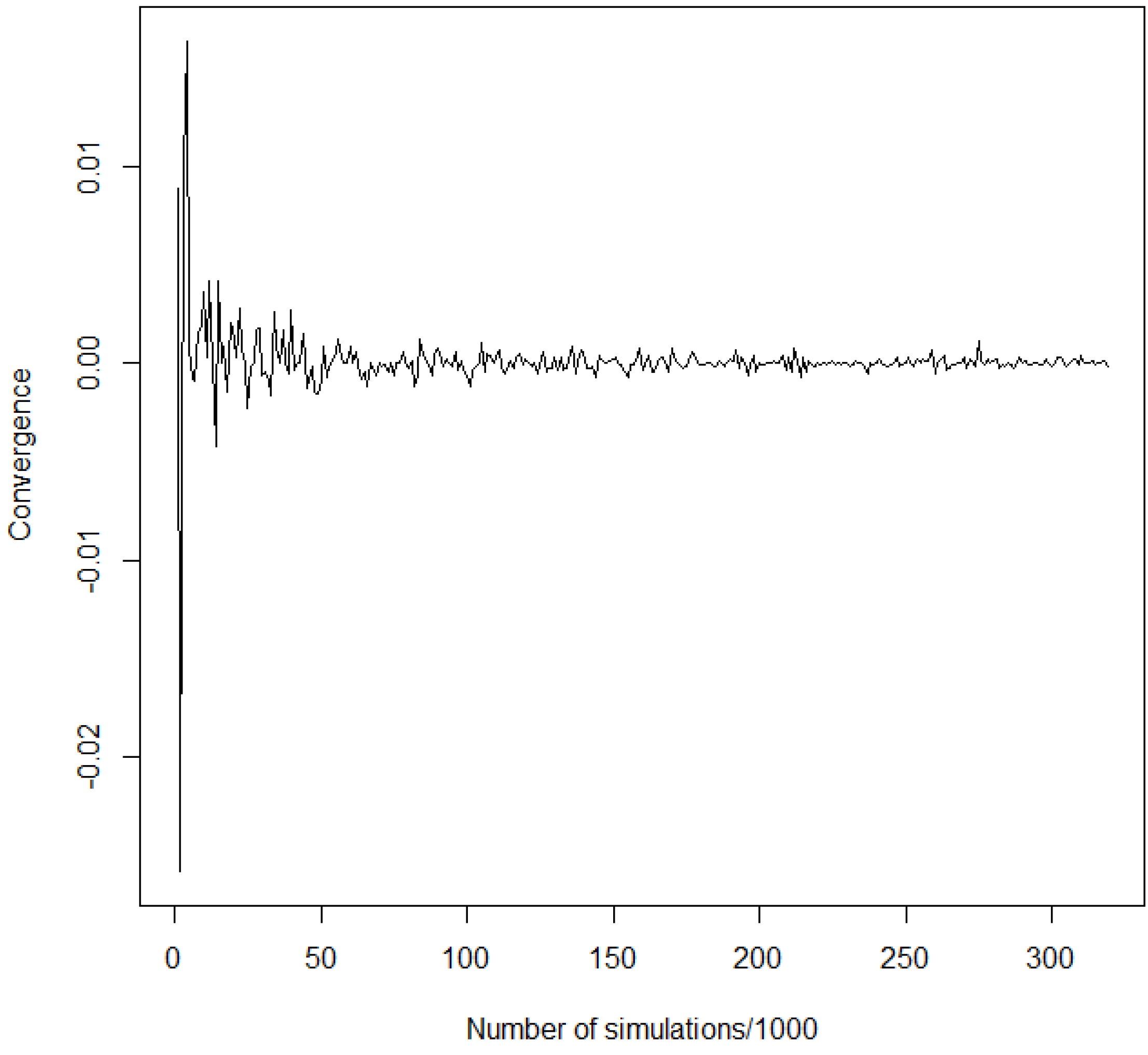
Given the parameters we estimated, we simulate losses with the algorithm in 4 and want to see the impact of our model of economic capital. The graphic in Figure 2 gives an idea of the convergence of economic capital for quantiles at 0.99.6

Figure 2. Convergence of quantiles at 0.99.

Figure 2. Convergence of quantiles at 0.99.

5.2. Results

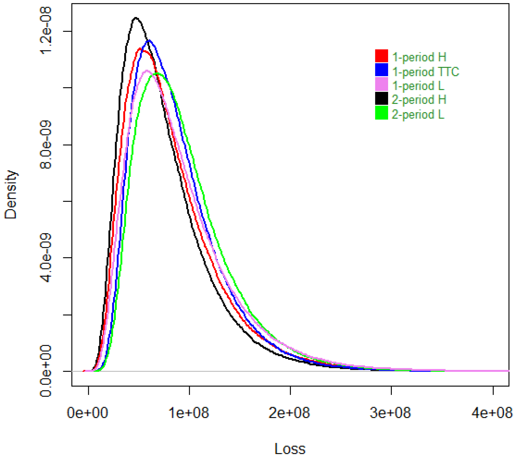
The annual loss densities in Figure 3 are obtained by simulating the two-period model. We compared the single-period model with three different hypothesis—one where we supposed that the cycle was high during the whole year, notated as 1 period H; another one when we were midway between a high and low cycle, notated as 1 period TTC; and finally, one where the cycle was low, notated as 1 period L—with the above two-period modeling, where the first period is more likely to be in a high cycle phase, notated as 2 period H, and the last case, where we suppose the first period is more likely to be a low cycle phase, notated as 2 period L.

Figure 3. The loss densities.

Figure 3. The loss densities.

The variations of economic capital for a quantile at 0.99, i.e., the loss quantile at 0.99 -the expected losses, are given in Table 1.

Table 1. Expected losses.

$\frac{\text{CE}\text{2}\text{period}\text{L}-\text{CE}\text{1}\text{period}\text{L}}{\text{CE}\text{1}\text{period}\text{L}}$	−9.3%
$\frac{\text{CE}\text{2}\text{period}\text{H}-\text{CE}\text{1}\text{period}\text{H}}{\text{CE}\text{1}\text{period}\text{H}}$	−1.8%
$\frac{\text{CE}\text{2}\text{period}\text{L}-\text{CE}\text{1}\text{period}\text{TTC}}{\text{CE}\text{1}\text{period}\text{TTC}}$	−3.9%
$\frac{\text{CE}\text{2}\text{period}\text{H}-\text{CE}\text{1}\text{period}\text{TTC}}{\text{CE}\text{1}\text{period}\text{TTC}}$	−9.6%

Table 1. Expected losses.

$\frac{\text{CE}\text{2}\text{period}\text{L}-\text{CE}\text{1}\text{period}\text{L}}{\text{CE}\text{1}\text{period}\text{L}}$	−9.3%
$\frac{\text{CE}\text{2}\text{period}\text{H}-\text{CE}\text{1}\text{period}\text{H}}{\text{CE}\text{1}\text{period}\text{H}}$	−1.8%
$\frac{\text{CE}\text{2}\text{period}\text{L}-\text{CE}\text{1}\text{period}\text{TTC}}{\text{CE}\text{1}\text{period}\text{TTC}}$	−3.9%
$\frac{\text{CE}\text{2}\text{period}\text{H}-\text{CE}\text{1}\text{period}\text{TTC}}{\text{CE}\text{1}\text{period}\text{TTC}}$	−9.6%

First, we observe that the economic capital computed with the two-period model is always lower than the one where losses are modeled with the single-period model.

In the case where the cycle is expected to be high during at least the first period, modeling losses with the two-period model will decrease the economic capital by 1.8% compared to the same hypothesis under the single-period model. This is due to the fact that in the second semester, there is a chance that the cycle is low, and in that case, the exposures of the insurer will decrease. When compared to the case of a single-period model, where the cycle has the same probability of being high or low (we call this the through-the-cycle), then the economic capital with the single period model goes down by 9.6%. This is coherent with what we expected.

When the cycle is expected to be low during the first semester, the two-period model of economic capital is lower by 9.3% compared to the one of the single-period, where the cycle is low during the whole year. When we compare this to the single-period economic capital under the through-the-cycle assumption, it is lowered by 3.9%. It is coherent to have a smaller decrease under the through-the-cycle assumption compared to the case where the cycle is low the whole year.

6. Conclusions

We presented in this paper a model considering business or credit cycles. This model is especially suited to credit insurance, because it predicts that the guarantees that the insurer offers can be decreased when the cycle is low and increased otherwise. The numerical application seems to tell us that the economic capital computed with our two-period model is lower than the one with one single period, which may be an appreciated feature. It also allows the insurer to better adapt its reserve level to the business cycle and to make less estimation errors than in a one-period model. Indeed, the more flexible model allows one to have reserves that better fit real needs.

The major difficulty in applying this model is finding the best discriminatory variable, which will help in distinguishing between cycle phases, and thus, different actions may be taken by the insurer. After finding this variable, Markov transition matrices should be estimated, in a consistent way. Applying the theory of hidden Markov chains to find a method to estimate these transition matrices will require further work.

References

- S. Koopman, and A. Lucas. “Business and Default Cycles for Credit Risk.” J. Appl. Econom. 20 (2005): 311–323. [Google Scholar] [CrossRef]
- S. Koopman, R. Kräussl, A. Lucas, and A. Monteiro. “Credit Cycles and Macro Fundamentals.” J. Empir. Financ. 16 (2009): 42–54. [Google Scholar] [CrossRef]
- F. Planchet, and J.F. Decroocq. “Systematic Risk Modelisation in Credit Risk Insurance.” In Proceedings of the Astin Colloquium, Helsinki, Finland, 1–4 June 2009.
- R. Merton. “An Analytic Derivation of the Cost of Deposit Insurance and Loan Guarantees an Application of Modern Option Pricing Theory.” J. Bank. Financ. 1 (1977): 3–11. [Google Scholar] [CrossRef]
- M. Crouhy, D. Galai, and R. Mark. “A Comparative Analysis of Current Credit Risk Models.” J. Bank. Financ. 24 (2000): 59–117. [Google Scholar] [CrossRef]
- M. Gordy. “A Risk-Factor Model Foundation for Ratings-Based Bank Capital Rules.” J. Financ. Intermed. 12 (2003): 199–232. [Google Scholar] [CrossRef]
- M. Gordy. “A Comparative Anatomy of Credit Risk Models.” J. Bank. Financ. 24 (2000): 119–149. [Google Scholar] [CrossRef]
- R. Frey, and A. McNeil. “Dependent Defaults in Models of Portfolio Credit Risk.” J. Risk 6 (2003): 59–92. [Google Scholar]
- R. Frey, A. McNeil, and M. Nyfeler. “Copulas and Credit Models.” Risk 10 (2001): 111–114. [Google Scholar]
- M. Pykhtin. “Portfolio Credit Risk Multi Factor Adjustment.” Lond. Risk Mag. Ltd. 17 (2004): 85–90. [Google Scholar]
- P. Schönbucher. Factor Models for Portfolio Credit Risk. Bonn, Germany: Department of Statistics, Bonn University, 2000. [Google Scholar]
- J. Gregory, and J. Laurent. “In the Core of Correlation.” Risk 17 (2004): 87–91. [Google Scholar]
- A. Bangia, F. Diebold, A. Kronimus, C. Schagen, and T. Schuermann. “Ratings Migration and the Business Cycle, with Application to Credit Portfolio Stress Testing.” J. Bank. Financ. 26 (2002): 445–474. [Google Scholar] [CrossRef]
- J. Hamilton. “A new Approach to the Economic Analysis of Nonstationary Time Series and the Business Cycle.” Econometrica 57 (1989): 357–384. [Google Scholar] [CrossRef]
- M. Hardy. “A Regime-Switching Model of Long-Term Stock Returns.” N. Am. Actuar. J. 5 (2001): 41–53. [Google Scholar] [CrossRef]
- J. Christensen, E. Hansen, and D. Lando. “Confidence Dets for Continuous-Time Rating Transition Probabilities.” J. Bank. Financ. 28 (2004): 2575–2602. [Google Scholar] [CrossRef]
- J. Gómez-González, and I. Hinojosa. “Estimation of Conditional Time-Homogeneous Credit Quality Transition Matrices.” Econ. Model. 27 (2010): 89–96. [Google Scholar] [CrossRef]
- Y. Jafry, and T. Schuermann. “Measurement, Estimation and Comparison of Credit Migration Matrices.” J. Bank. Financ. 28 (2004): 2603–2639. [Google Scholar] [CrossRef]
- P. Nickell, W. Perraudin, and S. Varotto. “Stability of Rating Transitions.” J. Bank. Financ. 24 (2000): 203–227. [Google Scholar] [CrossRef]
- D. Lando, and T. Skødeberg. “Analyzing Rating Transitions and Rating Drift with Continuous Observations.” J. Bank. Financ. 26 (2002): 423–444. [Google Scholar] [CrossRef]
Appendix
A. Kolmogorov’s Theorem
Theorem 2. Kolmogorov
Let be a sequence of independent random variables, such that:
- for all ,
- there exists a sequence, , of positive numbers that grows to , such that:
- 1.There is a default if the payment period lasts longer than was initially agreed upon by the insured and its client.
- 2.The maximum amount of money the insurer guarantees the insured in case of the default of his client, the buyer, n.
- 3.This will not be the final loss, because other contract clauses, such as reinsurance or deductibles, for example, will be taken into account. We will not consider those clauses in this paper.
- 4.This former case is modeled through the change in the UGD, whereas the latter is taken into account in the default probabilities. The reason for this is that in the case of the default of the buyer, when the guarantee has been canceled, the insurer pays nothing; this is as though the default never occurred from the insurer’s point of view.
- 5.We will assume here that the high (low) cycle phase is the period associated with a lower (higher) insolvency rate.
- 6.In the Solvency II directive it is recommended to compute quantiles at 0.995 for the economic capital estimation, but here, for practical issues and since it requires less simulations to converge, we chose to use the quantile at 0.99.
© 2014 by the authors; licensee MDPI, Basel, Switzerland. This article is an open access article distributed under the terms and conditions of the Creative Commons Attribution license (http://creativecommons.org/licenses/by/3.0/).
Share and Cite
MDPI and ACS Style
Caja, A.; Planchet, F. Modeling Cycle Dependence in Credit Insurance. Risks 2014, 2, 74-88. https://doi.org/10.3390/risks2010074
AMA Style
Caja A, Planchet F. Modeling Cycle Dependence in Credit Insurance. Risks. 2014; 2(1):74-88. https://doi.org/10.3390/risks2010074
Chicago/Turabian StyleCaja, Anisa, and Frédéric Planchet. 2014. "Modeling Cycle Dependence in Credit Insurance" Risks 2, no. 1: 74-88. https://doi.org/10.3390/risks2010074