Community Analysis of Global Financial Markets

Abstract

We analyze the daily returns of stock market indices and currencies of 56 countries over the period of 2002–2012. We build a network model consisting of two layers, one being the stock market indices and the other the foreign exchange markets. Synchronous and lagged correlations are used as measures of connectivity and causality among different parts of the global economic system for two different time intervals: non-crisis (2002–2006) and crisis (2007–2012) periods. We study community formations within the network to understand the influences and vulnerabilities of specific countries or groups of countries. We observe different behavior of the cross correlations and communities for crisis vs. non-crisis periods. For example, the overall correlation of stock markets increases during crisis while the overall correlation in the foreign exchange market and the correlation between stock and foreign exchange markets decrease, which leads to different community structures. We observe that the euro, while being central during the relatively calm period, loses its dominant role during crisis. Furthermore we discover that the troubled Eurozone countries, Portugal, Italy, Greece and Spain, form their own cluster during the crisis period.

1. Introduction

Financial crisis can cause substantial damages and economic losses not only locally, but also in other countries through trade relations, currency policies, financial contracts, and cross-country investments. Some examples of such crises are the 1997 Asian financial crisis, 1998 Russian bond crisis, 2001 dot-com bubble, 2007–2008 global financial crisis, and 2010 EU sovereign debt crisis, all spilling over to various parts of the world. Similar to the transmission of a disease, small financial shocks initially affecting only a particular sector of the economy or geographic region can spread to other economic sectors and other countries with quite healthy economic outlook [1].

Many research studies have examined the connections among countries by exploring correlations of various financial time series data [2,3,4,5,6,7,8,9,10,11,12,13,14,15,16,17,18,19,20,21,22,23]. Moreover, many studies have analyzed relationships between stock and foreign exchange markets, given the significant increase in global capital flows in the last two decades [24,25,26,27,28,29,30,31,32,33,34,35,36]. Other studies have focused on global stock market return predictability offering diverse findings across different regions and time periods [37,38,39,40,41,42,43,44,45,46,47].

There have been dramatic advances in the field of complex networks in many research fields. The world-wide-web, the Internet, highway systems, and electric power grids are all examples of networks that can be modeled using coupled systems [48,49,50,51,52,53,54,55], where the connectivity between network components is essential. Similarly, the economic system is composed of many agents, interacting at different levels. The agents in the system could be individual traders, firms, banks, financial markets, or countries, hence the global financial system can be well represented by using a complex network model. Recently, researchers have used network theory to study economic systems as well as systemic risk propagation through the financial network [56,57,58,59,60,61,62,63,64,65,66,67]. We develop and analyze a two-layer interdependent network, where each layer represents a different financial market and interactions exist not only within the same market, but also between the two layers. Because of these interdependences, failure in a certain network node can trigger global systemic risk and crisis propagation to other nodes in the network. In this study, we select major global stock market indices and their corresponding currencies as the two layers in our coupled network model.

Stock markets are a common trade place for company shares thus reflecting companies’ performances and investors’ perceptions of company values. Moreover, stock markets are considered leading economic indicators and therefore useful as predictors of the economy. The foreign exchange market is the largest financial market in the world, with market participants actively involved in currency trading 24 h a day except weekends, with daily turnover of over 5 trillion US dollars, according to the Bank for International Settlement [68]. These two financial markets capture important aspects of a country’s economic status, and therefore, we use them as a centerpiece of our research. We use a complex network approach to model the interaction between stock and foreign exchange markets to capture the topology as well as the dynamics in this coupled financial system. We study 56 stock market indices and 45 distinct currencies since 12 of the countries in our dataset use the euro as their official currency. Our analysis reveals novel insights and interesting features of the interactions among global stock and currency markets. We divide the entire period of 2002 to 2012 into two time intervals, non-crisis (2002–2006) and crisis (2007–2012) periods. We find that correlations exhibit different behavior during the crisis period such as higher stock market correlations and lower foreign exchange correlations when compared to the non-crisis period.

The objective of this article is to study community formations in global financial markets and to investigate the systemic importance of countries and their influence on other countries or regions. The rest of the paper is organized as follows: In Section 2, we present our correlation-based community analysis results for two different sub-periods, non-crisis period (2002–2006) and crisis period (2007–2012); in Section 3, we offer a discussion of our findings. The data set and the methods we use are described in Section 4.

2. Results

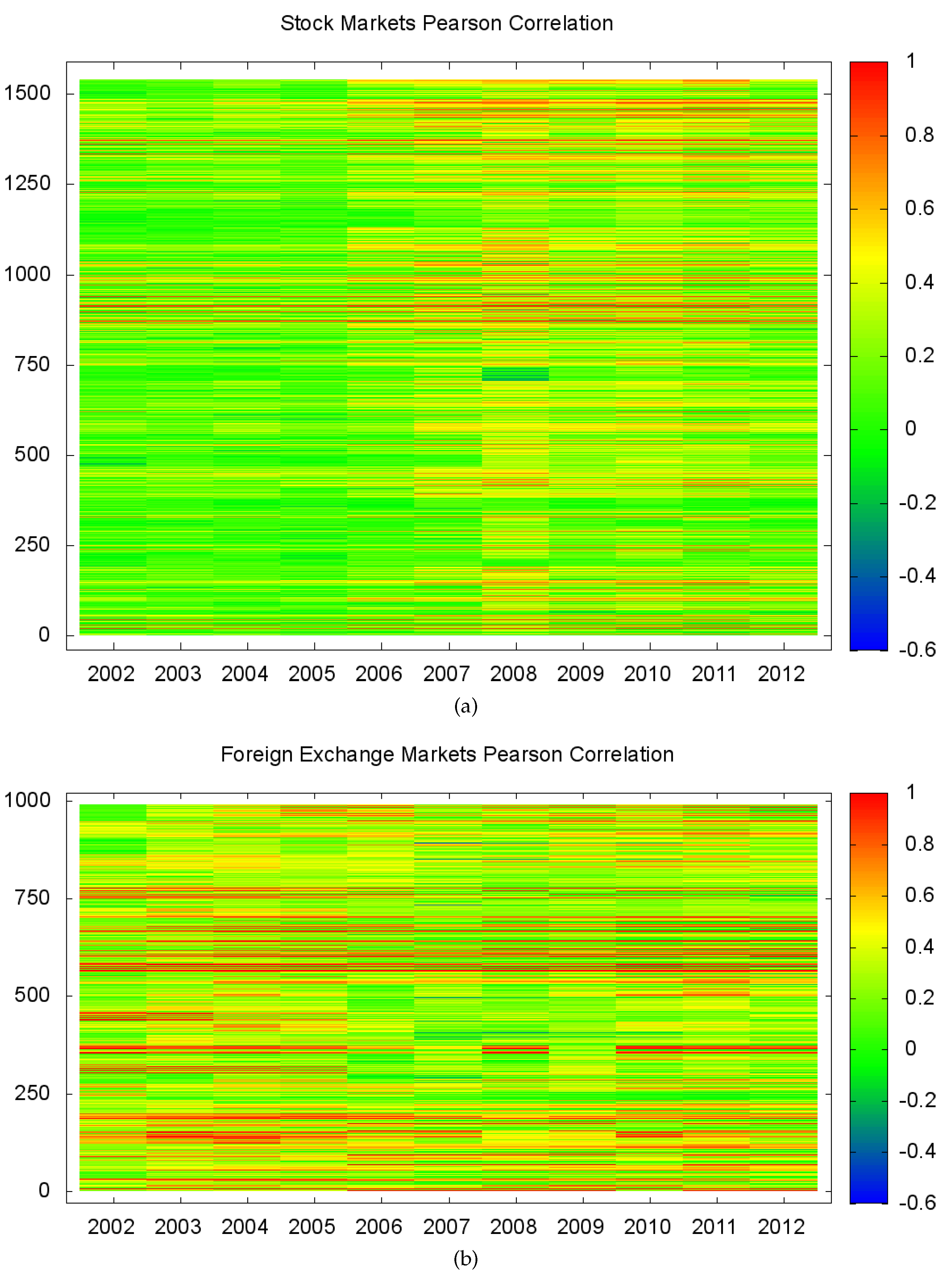
2.1. Pearson Correlation Analysis

In order to see how the cross-correlation trends change with time, we divide the data into 11 annual periods. Figure 1a shows a heat map of the yearly stock market correlations. The x-axis represents the years, and the y-axis shows the 1540 unique pairwise correlations, excluding the diagonal of the correlation matrix. We use the color bar to show the magnitude of the correlations, where red means $C=1$ and the two series are perfectly positively correlated, while blue means $C=-1$ and the two series are perfectly negatively correlated. Green means $C=0$, or the two series are not correlated.

From Figure 1a, we can see that the overall correlation of the global stock markets trends upward starting in 2006, reaches its peak in 2008, and stays at a high level thereafter. These increasing correlation trends match the global financial crisis of 2007–2008 and could possibly be regarded as indicators of increased co-movements heading towards financial crisis.

In Figure 1b, the heat map for foreign exchange markets is plotted. It is generated in the same way as the heat map for the stock markets; however, the number of entries is lower due to the lower number (45) of distinct currencies among the 56 countries. Hence, we have 990 distinct correlations for the currency correlation matrix, excluding the diagonal. Generally, foreign exchange markets shows stronger correlation compared to stock markets. It seems that the overall foreign exchange correlation falls during the financial crisis period, contrary to the stock market correlation trend.

2.2. Summary Statistics

To study the statistical characteristics of the correlations, we calculate the first moment (mean) and the second moment (standard deviation) of any of the correlation distributions for the 11 years for all three cases, including Pearson correlations for stock market layer, currency layer, as well as inter-layer correlations.

In Figure 2, we show that the mean value of stock market correlations exhibits a peak during the crisis period (2007–2012). This finding suggests (similar to Figure 1a) that during crisis, the overall correlation increases, and the stock markets tend to move together. This could be due to portfolio re-balancing, reducing equity market exposures and increasing allocations in the bond market. The re-balancing in global portfolios occurs across different countries and thus produces declining stock market trends internationally.

The means of the foreign exchange market Pearson correlations are low during the crisis period, while, in contrast, we observe a peak during the non-crisis period. This finding suggests that, in general, the correlations among currencies are low during crises and high during non-crisis periods, contrary to the stock market behavior. For both, however, the standard deviation of the correlations remains fairly constant, which suggests uniform increase (decrease) of the correlations in the stock markets (foreign exchange markets) throughout the entire time period.

In order to confirm this qualitative description that the means of the correlation are in fact different for the years in the calm period and for the years in the crisis period, we perform Student’s t-test. The null hypothesis is that the annual mean correlations are the same for both periods and that any differences come from the standard deviation. We apply the two-sample Student’s t-test. It rejects the null hypothesis that the two means are equal, p-value is $0.0002$; thus, the alternative hypothesis that the means are not equal is accepted.

The mean value of Pearson correlations between stock and foreign exchange markets exhibits a local minimum during the crisis period, which could be interpreted as positive stock market returns corresponding to currency appreciations. Overall the interlayer correlation does not change much throughout the entire period. The increase in standard deviation, however, indicates a larger spread in correlation values between the two layers during the crisis (

Table 1. Statistics for the pre-crisis and the crisis periods.

	Stocks		Currency
	2002–2006	2007–2012	2002–2006	2007–2012
Mean	$0.175$	$0.315$	$0.370$	$0.318$
Standard Deviation	$0.208$	$0.249$	$0.260$	$0.279$
Minimum	$-0.320$	$-0.340$	$-0.155$	$-0.575$
Maximum	$0.965$	$0.966$	$1.000$	$1.000$

).

We distinguish between two different markets in our analysis, the network of stock market indices and the network of foreign exchange markets. Besides their obvious differences, the two markets also exhibit different correlation distributions, as visual inspection of Figure 1a,b hints. The two-sample Kolmogorov-Smirnov test (K-S test) allows us to statistically confirms this, with the null hypothesis being that the two sample data are from the same continuous distribution. The K-S test rejects this null hypothesis at a significance level $\alpha =0.001$. Therefore, we can conclude that the correlation distributions of stock markets and of foreign exchange markets are different.

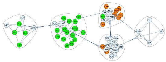
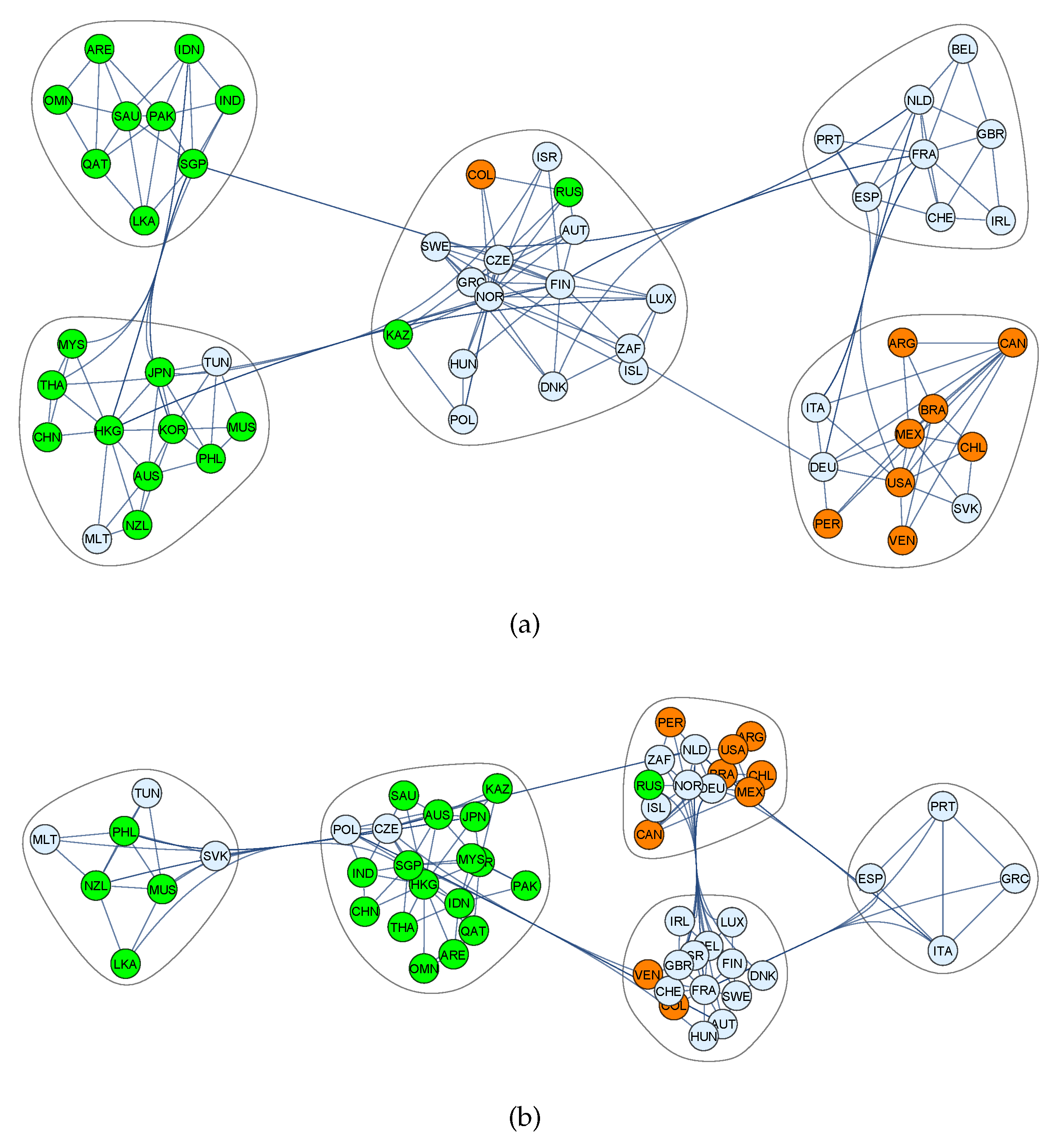
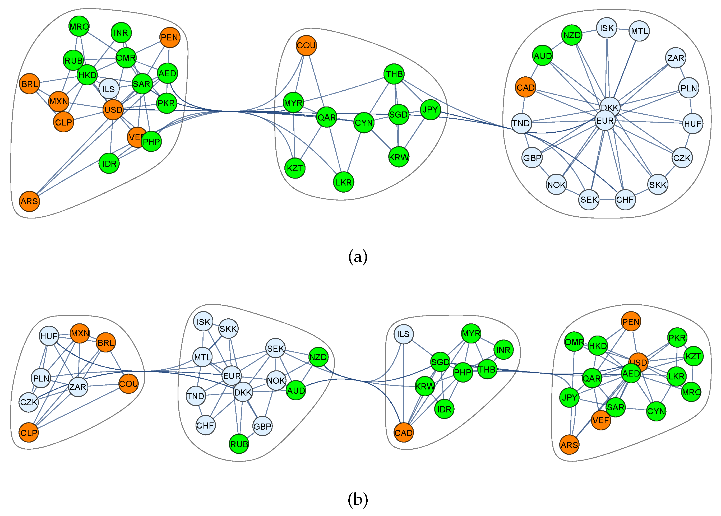
2.3. Community Formation and Cluster Analysis

In our analysis we focus on two periods: a period of relative economic calmness (2002–2006) and a period of economic crisis (2007–2012). Using the correlation information, we depict the network structure of the stock markets and of the foreign exchange markets for each of these time periods. Since countries have different peak trading times due to their respective geographical locations and different time zones, lagged correlations allow us to infer information about regional influences. We separate the 56 countries and 45 currencies into three groups according to their geographical location. When we consider synchronous correlations, we use the returns at time t for every country. In that case, the Asian markets are the first to trade, then the European markets, and finally the American markets. A shock originating in the US, for example, would then not show its immediate effect on the other markets because the stock markets in other parts of the world are closed for most or all of the trading hours of the NYSE. When we consider lagged correlations, we use the returns at time t for the American countries and at time $t+1$ for the other countries of the world. In that case, it is as if the American markets were first to trade, followed by the Asian and then the European markets. A shock from the US would then be very visible. For both, the stock and the foreign exchange markets, we first consider the synchronous correlations and then compare the results to those of the lagged correlations.

We use Planar Maximally Filtered Graphs (PMFG) [69,70] to study the properties of stock and foreign exchange market correlations. PMFG is useful for filtering meaningful correlations from the bulk of the 1540 correlation pairs, as it suppresses small correlations while maintaining the overall network structure. In order to build the graph, we order the correlations $C_{i,j}$ from largest to smallest. First, the pair with the largest correlation is connected. In subsequent steps we connect the countries $i,j$ under the condition that a link between them maintains the planar structure of the graph; if it does not, the pair is skipped. This procedure results in an adjacency matrix with unweighted links from which the graph is plotted. We use Wolfram Mathematica to investigate the communities in the network, which are detected with respect to their modularity.

2.3.1. Stock Markets

Synchronous Correlations

Figure 3a shows the PMFG for the period from 2002 to 2006, where we identify five clusters which seem to be organized by geographical locations. The cluster on the top left is led by Singapore, a financial hub, and Saudi Arabia, which connects to many other OPEC countries in the cluster. The second Asian cluster is centered around Hong Kong and Japan. The third cluster contains smaller European countries, organized around the Scandinavian countries. The fourth cluster contains the major European economies, except for Italy and Germany which are closely connected to the American countries in the fifth cluster, particularly through ties to the US and Canada. These four countries exhibit particularly strong connections within and, in case of Germany and Italy, to countries outside the cluster. The communities change significantly during the crisis period, where Singapore and Hong Kong lead a large Asian cluster, as illustrated in Figure 3b. The American cluster formed during the non-crisis period becomes more mixed during the crisis period, as Norway, Iceland and Russia become part of this cluster. The change in the community comprised of mostly American countries suggest that Italy and Germany influence the performance of the American markets in the non-crisis period, while during the crisis period, Norway and Russia seem to increase their influence. The majority of the European countries, connected through France, form another cluster, strongly linked to the countries in the American cluster. These observations are in line with the coordinated responses to the crisis from the US, large European economies, and the ECB; at the same time the Asian countries do not become more closely connected to them [71]. Most notably, however, two new clusters appear: one with the troubled Eurozone countries Portugal, Italy, Greece and Spain, and another consisting of rather less connected countries like Slovakia, Mauritius and Tunisia.

Lagged Correlations

As pointed out before, lagged correlations are an important measure to study the influences of financial markets. They allow us to consider effects originating in one region and spreading to another. In the following, we consider the correlation calculated for the returns for the Americas at time t, and for Asia and Europe at time $t+1$. In other words, we focus on how the index movements in the Americas will affect the index movements in the rest of the world. Please note that this does not change the correlations within one geographical region, nor will the correlations between Asian and European countries change. However, due to the PMFG algorithm, larger correlations that appear for countries in the Americas with countries in the rest of the world can change the structure of the network.

The European clusters remain mostly unchanged in the calm period, except that Germany and Italy no longer form a community with American countries, when considering lagged correlations compared to synchronous correlations. Since here we consider the Americas at time t and Europe and Asia at time $t+1$, it seems that the American countries, including the US, do not affect Italy and Germany significantly. The Netherlands, Italy, France, and the Scandinavian countries still manifest themselves as the most connected European countries. We do, however, observe large changes in the American cluster on the very right in Figure 4a; Australia and New Zealand, economically close to the US, have moved from the Asian community to connect more tightly to the American countries. Different responses by central banks, leading to higher interest rates particularly in Australia, can be considered a reason for this [72]. They are joined by smaller countries, such as Sri Lanka and the Philippines, that we have previously identified as countries with weak links to other Asian countries. The Asian cluster is led by Singapore, Hong Kong and Japan, which display the most significant correlations to countries outside of their community. The community structure changes significantly when we consider the years of economic turmoil in Figure 4b. Most obviously, the number of communities reduces to three because the two European clusters from the non-crisis period mostly merge. Netherlands, United Kingdom and France are at the center of the European community in the crisis period. Portugal, Italy, Greece and Spain are found at the periphery of this cluster. Using synchronous correlations, Germany and Netherlands were tightly connected to the American cluster during the crisis period, while when considering lagged correlations, they belong to the large European cluster. We observe that Japan, Australia and New Zealand, among others, form a community with the American countries during the crisis, which suggests that the major financial markets in the Pacific follow the trends of the American stock markets. The importance of the US stock market is emphasized by the largest number of connections in this cluster. Australia is the second most connected country in this community.

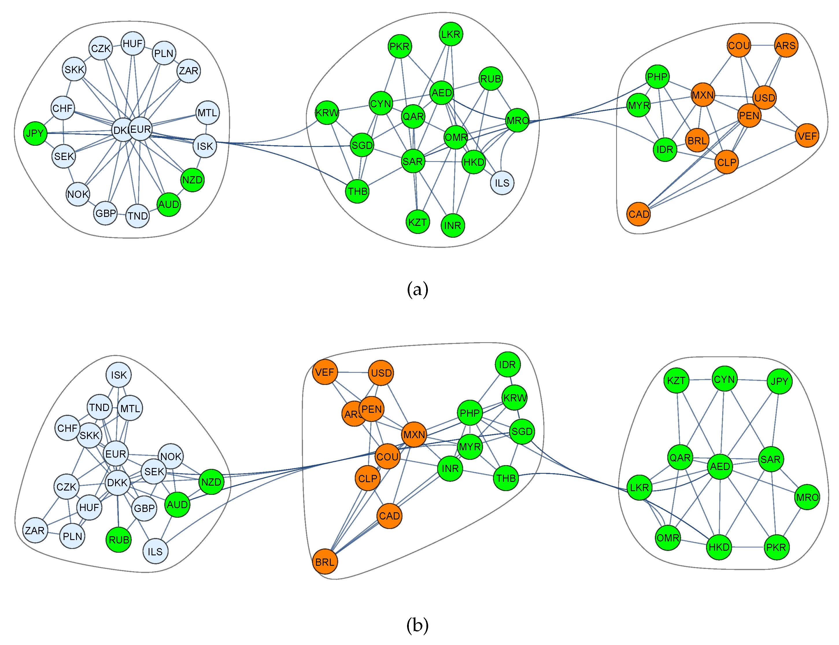
2.3.2. Foreign Exchange Markets

While we analyze a total of 56 global stock market indices, we only investigate 45 currencies because 12 countries use the euro.

Synchronous Correlations

Figure 5a shows the dominant role that the euro has played in Europe prior to the crisis. Together with the Danish krone, pegged to the euro via the European Exchange Rate Mechanism, the euro is connected with all European currencies, and it exhibits close ties to the Canadian dollar, the Australian dollar, and the New Zealand dollar. With 19 links each, the node for the euro and the node for the US dollar show the highest interconnectedness among all currencies in the calm period. The US dollar is at the center of the cluster comprised of the majority of the American currencies and the oil-exporting countries. In Figure 5b we observe that the clear structure and hierarchy of the European community during the calm period falls apart during crisis. In addition, a fourth cluster appears, comprised of European and South and Central American currencies, like the Brazilian real, the Mexican peso and the Chilean peso, which were closely connected to the US dollar in the non-crisis period. As the financial crises unfolded, the Fed and its European counterparts employed “quantitative easing” as monetary policy, which in turn has been eliciting strong criticism in the BRIC countries, as QE corresponds to currency devaluation [73]. The US dollar maintains its strong ties with the currencies of oil-exporting countries. Its cluster is joined by the Japanese yen and the Chinese yuan. China moved to a managed floating regime during the crisis period [74], whereas the Japanese government tried to stimulate its economy with policies similar to QE, known as “Abenomics” [75].

Lagged Correlations

In Figure 6a, using lagged correlations during the non-crisis period, we observe that the Euro is at the center of the cluster of European currencies. The Japanese yen joins this cluster. The US dollar and the currencies of the Asian (Middle Eastern) oil-exporting countries no longer share close ties. We notice in Figure 6b, during the crisis period, that there is a mixed cluster comprised of all the American currencies and a group of Asian currencies, including India, Singapore and Korea, while the South East Asian currencies form their own community using synchronous correlations, as observed in Figure 5b. The number of connections of the nodes comparing the two different periods remains stable; the majority of the currencies do not gain or lose more than two connections. Instead we find that different connections develop within the clusters. For example, Hong Kong loses the link with countries like India and Russia during the crisis, but becomes more closely connected to Singapore, the Philippines and Thailand.

Any currency is traded during every hour of the day, therefore any sudden changes should be reflected in all the currencies on a time scale shorter than one full day. In fact, one would expect the strong correlations to correspond to shorter time scales. Hence the community structure of the currencies is depicted by synchronous correlations, while when using lagged correlations, the true structure of the network disappears.

3. Discussion

In this study, we investigate the daily logarithmic returns in the stock and foreign exchange markets of 56 countries and 45 currencies. We use network theory and community analysis to understand the structure of the coupled financial network formed by global stock market indices and currencies. We define weighted links within a network layer and between the two layers (stock markets on one hand and currencies on the other) using Pearson correlation. The overall correlations within stock markets increase during the crisis period, and the overall correlations within foreign exchange markets, as well as the correlations between stock and foreign exchange markets decrease during this period. We investigate statistical properties of our results by presenting correlation summary statistics and performing the K-S test to closely study the characteristics of the correlation distributions. We apply the PFMG method to discover distinct community formations and categorize the countries into clusters. We identify the importance of the countries according to their relative positions in the communities and the strength of their links with other member of the community as well as the strength of their external links with countries that do not belong to their cluster. In our analysis, we distinguish between synchronous and lagged correlations. We divide the countries in three geographical regions, Asia, Europe and Americas. To study lagged correlations, we consider the returns at time t in the Americas, and the returns at time $t+1$ in Asia and Europe. The comparison of the network and community structures allows us to infer influences from one region to another, in both, crisis and non-crisis periods. Using synchronous correlations we identify five clusters in the stock market during the non-crisis period. These clusters change their structure during the crisis period, where, for example, four of the five troubled Eurozone countries, Portugal, Italy, Spain and Greece, form their own community. In the case of lagged correlations, we observe four clusters in the stock market layer during the non-period period and only three communities during the crisis period. We observe that the American countries are most closely connected to Asian countries. The introduction of a time lag and the onset of the crisis cause the European countries to become more tightly connected. Unlike stock markets, which are bound to different time zones, currencies trade around the clock. Any influences among currencies are immediately reflected in their returns, hence synchronous correlation define the true network structure of the foreign exchange markets. We observe that the Euro plays a central role among the European currencies during the non-crisis period, while it loses its central position during the crisis-period. The US dollar is closely linked to the currencies of the major oil-exporting countries, both, during non-crisis and crisis periods.

These findings could have policy implications and could be helpful for central bankers, policy makers and regulators, offering a tool for identifying tightly related communities of countries by stock market performance and by currency dynamics. If, for instance, a financial crisis originates in a specific country, the most vulnerable countries, where the crisis might spread first, are the countries with stronger links with the originating country, most likely belonging to the same community. If policy makers have knowledge of these communities, they might be able to focus needed bailout funds or implement temporary preventative measures in the most vulnerable countries, thus reducing the impact of inherent global financial crisis to the rest of the world and preventing the propagation of the crisis before severe damages cripple the entire economic system.

4. Materials and Methods

4.1. Data

We acquired the data from the Boston University Bloomberg terminal provided by Bloomberg L.P. for academic research. In our analyss, we use a time range of 11 years from January 1, 2002 to December 31, 2012, with daily frequency. We use the daily closing price. We exclude the weekends, and for holidays we repeat the closing price of the previous day. We select 56 representative countries, which include developed as well as emerging countries.

When a country has more than one well-known major stock market index, we use the following criteria to select the most representative index: first we select the stock market indices that are widely used in the financial industry, and from that subset, we select the index that includes most of the companies listed on the respective exchange, covering mostly large capitalization stocks but in some instances including some mid or small capitalization stocks as well. Using this criteria, we have selected one single index for each country, such as the S&P 500 for the US, Nikkei 225 for Japan, STI for Singapore, etc.

For the foreign exchange rates, we use the closing mid price, which is the average of the closing bid and ask prices. The foreign exchange market convention is for the majority of the currencies to be expressed in terms of USD, except for the British pound, Australian dollar, New Zealand dollar, and the euro that are expressed as USD per currency. In our analysis, for consistency, we have converted these four currencies to be expressed in terms of USD. For any country in the eurozone that has adopted the euro at a later date than January 1, 2002, we keep the separate currencies up to the date before the actual euro adoption, and replace them with euro after the adoption day. This is becuase before the adoption of the euro, these currencies moved independently from the euro to some extent [76,77]. Examples like these include the Maltese lira and Slovak koruna, which were replaced by the euro on January 1, 2008 and January 1, 2009 respectively.

In order to also include the US dollar as part of our analysis, we have expressed all currencies as currency over SDR. The SDR is an international reserve asset, created by the International Monetary Fund (IMF) in 1969 to supplement its member countries’ official reserves. Its value is based on a basket of four key international currencies, and SDRs can be exchanged for freely usable currencies. Though it is not a currency, per se the SDR can be used as a currency unit in our study [78,79]. The IMF fixes the value of one SDR in terms of US dollars daily.

4.2. Pearson Correlation Analysis

For all analyzed time-series, we first obtain the logarithmic returns as follows. $P\left(t\right)$ is the value of the time series at time t, where $t=1,2,\cdots ,N$, and $N=2866\mathrm{days}$ is the size of the time series. The logarithmic return of time series i is

$$R_i\left(t\right)=ln\frac{P_i(t+1)}{P_i\left(t\right)}$$

(1)

We then normalize $R_i\left(t\right)$ to have zero mean and unit standard deviation,

$$r_i\left(t\right)=\frac{R_i\left(t\right)-\overline{R_i}}{{\sigma }_{R_i}}$$

(2)

where $\overline{R_i}$ and ${\sigma }_{R_i}$ are the mean value and standard deviation of time series i.

For stock market indices, the dimension of the logarithmic return time series matrices is $56\times 2865$. For foreign exchange markets, it is $45\times 2865$ since we group all Eurozone countries together. We calculate the cross-correlation matrix C, and the value of each cell $C_{i,j}$ as follows,

$$C_{i,j}=\langle r_i{r}_j\rangle$$

(3)

where $C_{i,j}$ represents the Pearson correlation between logarithmic return time series for a pair of countries i and j.

4.3. Analyzed Countries

Country	Currency	Index Label	Currency Label	Country	Currency	Index Label	Currency Label
Argentina	Argentine peso	ARG	ARS	Malta	Maltese lira	MLT	MTL/EUR
Australia	Australian dollar	AUS	AUD	Mauritius	Mauritian rupee	MUS	MRO
Austria	euro	AUT	EUR	Mexico	Mexican peso	MEX	MXN
Belgium	euro	BEL	EUR	Netherlands	euro	NLD	EUR
Brazil	Brazilian real	BRA	BRL	New Zealand	New Zealand dollar	NZL	NZD
Canada	Canadian dollar	CAN	CAD	Norway	Norwegian krone	NOR	NOK
Chile	Chilean peso	CHL	CLP	Oman	Omani rial	OMN	OMR
China	Chinese yuan	CHN	CNY	Pakistan	Pakistani rupee	PAK	PKR
Colombia	Colombian peso	COL	COU	Peru	Peruvian nuevo sol	PER	PEN
Czech Republic	Czech koruna	CZE	CZK	Philippines	Philippine peso	PHL	PHP
Denmark	Danish krone	DNK	DKK	Poland	Polish zloty	POL	PLN
Finland	euro	FIN	EUR	Portugal	euro	PRT	EUR
France	euro	FRA	EUR	Qatar	Qatari riyal	QAT	QAR
Germany	euro	DEU	EUR	Russia	Russian ruble	RUS	RUB
Greece	euro	GRC	EUR	Saudi Arabia	Saudi riyal	SAU	SAR
Hong Kong	Hong Kong dollar	HKG	HKD	Singapore	Singapore doller	SGP	SGD
Hungary	Hungarian forint	HUN	HUF	Slovakia	Slovak koruna	SVK	SKK/EUR
Iceland	Icelandic krona	ISL	ISK	South Africa	South African rand	ZAF	ZAR
India	Indian rupee	IND	INR	Spain	euro	ESP	EUR
Indonesia	Indonesian rupiah	IDN	IDR	Sri Lanka	Sri Lankan rupee	LKA	LKR
Ireland	euro	IRL	EUR	Sweden	Swedish krona	SWE	SEK
Israel	Israel new shekel	ISR	ILS	Switzerland	Swiss franc	CHE	CHF
Italy	euro	ITA	EUR	Thailand	Thai baht	THA	THB
Japan	Japanese yen	JPN	JPY	Tunisia	Tunisian dinar	TUN	TND
Kazakhstan	Kazakhstani tenge	KAZ	KZT	Utd. Arab Emirates	UAE dirham	ARE	AED
Korea	South Korean won	KOR	KRW	United Kingdom	British pound	GBR	GBP
Luxembourg	euro	LUX	EUR	United States	US dollar	USA	USD
Malaysia	Malaysian ringgit	MYS	MYR	Venezuela	Venezuelan bolivar	VEN	VEF

References

1. W.L. Lin, R.F. Engle, and T. Ito. “Do Bulls and Bears Move Across Borders? International Transmission of Stock Returns and Volatility as the World Turns.” Rev. Financ. Stud. 7 (1994): 507–538. [Google Scholar] [CrossRef]
2. R.D. Smith. “The spread of the credit crisis: View from a stock correlation network.” J. Korean Phys. Soc. 54 (2009): 2460–2463. [Google Scholar] [CrossRef] [Green Version]
3. K.J. Forbes, and R. Rigobon. “No contagion, only interdependence: Measuring stock market comovements.” J. Financ. 57 (2002): 2223–2261. [Google Scholar] [CrossRef]
4. T.J. Flavin, M.J. Hurley, and F. Rousseau. “Explaining stock market correlation: A gravity model approach.” Manch. Sch. 70 (2002): 87–106. [Google Scholar] [CrossRef]
5. B. Solnik, C. Boucrelle, and Y. Le Fur. “International market correlation and volatility.” Financ. Anal. J. 52 (1996): 17–34. [Google Scholar] [CrossRef]
6. L. Ramchand, and R. Susmel. “Volatility and cross correlation across major stock markets.” J. Empir. Financ. 5 (1998): 397–416. [Google Scholar] [CrossRef]
7. B.H. Boyer, T. Kumagai, and K. Yuan. “How do crises spread? Evidence from accessible and inaccessible stock indices.” J. Financ. 61 (2006): 957–1003. [Google Scholar] [CrossRef]
8. G. Bonanno, N. Vandewalle, and R.N. Mantegna. “Taxonomy of stock market indices.” Phys. Rev. E 62 (2000): R7615–R7618. [Google Scholar] [CrossRef]
9. G. Bonanno, G. Caldarelli, F. Lillo, and R.N. Mantegna. “Topology of correlation-based minimal spanning trees in real and model markets.” Phys. Rev. E 68 (2003): 046130. [Google Scholar] [CrossRef] [PubMed]
10. G. Bonanno, G. Caldarelli, F. Lillo, F. Miccichè, N. Vandewalle, and R.N. Mantegna. “Networks of equities in financial markets.” Eur. Phys. J. B 38 (2004): 363–371. [Google Scholar] [CrossRef]
11. E. Sheedy. “Correlation in currency markets a risk-adjusted perspective.” J. Int. Financ. Mark. Inst. Money 8 (1998): 59–82. [Google Scholar] [CrossRef]
12. R. Meese. “Currency fluctuations in the post-Bretton Woods era.” J. Econ. Perspect. 4 (1990): 117–134. [Google Scholar] [CrossRef]
13. F. Longin, and B. Solnik. “Is the correlation in international equity returns constant: 1960–1990.” J. Int. Money Financ. 14 (1995): 3–26. [Google Scholar] [CrossRef]
14. B. Arshanapalli, and J. Doukas. “International stock market linkages: Evidence from the pre-and post-October 1987 period.” J. Bank. Financ. 17 (1993): 193–208. [Google Scholar] [CrossRef]
15. D.Y. Kenett, Y. Shapira, A. Madi, S. Bransburg-Zabary, G. Gur-Gershgoren, and E. Ben-Jacob. “Dynamics of stock market correlations.” AUCO Czech Econ. Rev. 4 (2010): 330–341. [Google Scholar]
16. D.Y. Kenett, Y. Shapira, A. Madi, S. Bransburg-Zabary, G. Gur-Gershgoren, and E. Ben-Jacob. “Index cohesive force analysis reveals that the US market became prone to systemic collapses since 2002.” PLoS ONE 6 (2011): e19378. [Google Scholar] [CrossRef] [PubMed]
17. D.Y. Kenett, M. Raddant, T. Lux, and E. Ben-Jacob. “Evolvement of uniformity and volatility in the stressed global financial village.” PLoS ONE 7 (2012): e31144. [Google Scholar] [CrossRef] [PubMed]
18. J.P. Onnela, A. Chakraborti, K. Kaski, J. Kertesz, and A. Kanto. “Dynamics of market correlations: Taxonomy and portfolio analysis.” Rev. Mod. Phys. 68 (2003): 056110. [Google Scholar] [CrossRef] [PubMed]
19. L. Sandoval, and I.D.P. Franca. “Correlation of financial markets in times of crisis.” Phys. A Stat. Mech. Appl. 391 (2012): 187–208. [Google Scholar] [CrossRef]
20. L. Sandoval. “To lag or not to lag? How to compare indices of stock markets that operate on different times.” Phys. A Stat. Mech. Appl. 403 (2014): 227–243. [Google Scholar] [CrossRef]
21. C. Curme, M. Tumminello, R.N. Mantegna, H.E. Stanley, and D.Y. Kenett. “Emergence of statistically validated financial intraday lead-lag relationships.” SSRN Electron. J. 15 (2015): 1375–1386. [Google Scholar] [CrossRef]
22. T. Aste, W. Shaw, and T. Di Matteo. “Correlation structure and dynamics in volatile markets.” New J. Phys. 12 (2010): 085009. [Google Scholar] [CrossRef]
23. M. Tumminello, T. Di Matteo, T. Aste, and R.N. Mantegna. “Correlation based networks of equity returns sampled at different time horizons.” Eur. Phys. J. B 55 (2007): 209–217. [Google Scholar] [CrossRef]
24. R. Dornbusch, and S. Fischer. “Exchange rates and the current account.” Am. Econ. Rev. 70 (1980): 960–971. [Google Scholar]
25. M. Dooley, and P. Isard. “A portfolio-balance rational-expectations model of the dollar-mark exchange rate.” J. Int. Econ. 12 (1982): 257–276. [Google Scholar] [CrossRef]
26. B. Morley. “Exchange rates and stock prices: Implications for European convergence.” J. Policy Model. 24 (2002): 523–526. [Google Scholar] [CrossRef]
27. C.C. Nieh, and C.F. Lee. “Dynamic relationship between stock prices and exchange rates for G-7 countries.” Q. Rev. Econ. Financ. 41 (2002): 477–490. [Google Scholar] [CrossRef]
28. K.H. Bae, G.A. Karolyi, and R.M. Stulz. “A new approach to measuring financial contagion.” Rev. Financ. Stud. 16 (2003): 717–763. [Google Scholar] [CrossRef]
29. L. Gagnon, and G.A. Karolyi. “Price and volatility transmission across borders.” Financ. Mark. Inst. Instrum. 15 (2006): 107–158. [Google Scholar] [CrossRef]
30. L. Cappiello, and R.A. De Santis. Explaining Exchange Rate Dynamics: The Uncovered Equity Return Parity Condition. ECB Working Paper. 2005. Available online: http://ssrn.com/abstract=804924 (accessed on 19 October 2005).
31. C.W. Granger, B.N. Huangb, and C.W. Yang. “A bivariate causality between stock prices and exchange rates: Evidence from recent Asianflu*.” Q. Rev. Econ. Financ. 40 (2000): 337–354. [Google Scholar] [CrossRef]
32. M.S. Pan, R.C.W. Fok, and Y.A. Liu. “Dynamic linkages between exchange rates and stock prices: Evidence from East Asian markets.” Int. Rev. Econ. Financ. 16 (2007): 503–520. [Google Scholar] [CrossRef]
33. C. Ning. “Dependence structure between the equity market and the foreign exchange market—A copula approach.” J. Int. Money Financ. 29 (2010): 743–759. [Google Scholar] [CrossRef]
34. H. Zhao. “Dynamic relationship between exchange rate and stock price: Evidence from China.” Res. Int. Bus. Financ. 24 (2010): 103–112. [Google Scholar] [CrossRef]
35. G. Katechos. “On the relationship between exchange rates and equity returns: A new approach.” J. Int. Financ. Mark. Inst. Money 21 (2011): 550–559. [Google Scholar] [CrossRef]
36. C.H. Lin. “The comovement between exchange rates and stock prices in the Asian emerging markets.” Int. Rev. Econ. Financ. 22 (2012): 161–172. [Google Scholar] [CrossRef]
37. L. Cohen, and A. Frazzini. “Economic links and predictable returns.” J. Financ. 63 (2008): 1977–2011. [Google Scholar] [CrossRef]
38. J.H. Cochrane. “The dog that did not bark: A defense of return predictability.” Rev. Financ. Stud. 21 (2008): 1533–1575. [Google Scholar] [CrossRef]
39. E.F. Fama, and K.R. French. “Dividend yields and expected stock returns.” J. Financ. Econ. 22 (1988): 3–25. [Google Scholar] [CrossRef]
40. E.F. Fama, and K.R. French. “Business conditions and expected returns on stocks and bonds.” J. Financ. Econ. 25 (1989): 23–49. [Google Scholar] [CrossRef]
41. I. Welch, and A. Goyal. “A comprehensive look at the empirical performance of equity premium prediction.” Rev. Financ. Stud. 21 (2008): 1455–1508. [Google Scholar] [CrossRef]
42. W.E. Ferson, and C.R. Harvey. “The risk and predictability of international equity returns.” Rev. Financ. Stud. 6 (1993): 527–566. [Google Scholar] [CrossRef]
43. M. Dahlquist, and H. Hasseltoft. “International bond risk premia.” J. Int. Econ. 90 (2013): 17–32. [Google Scholar] [CrossRef] [Green Version]
44. W. Breen, L.R. Glosten, and R. Jagannathan. “Economic significance of predictable variations in stock index returns.” J. Financ. 44 (1989): 1177–1189. [Google Scholar] [CrossRef]
45. C.R. Harvey. “The world price of covariance risk.” J. Financ. 46 (1991): 111–157. [Google Scholar] [CrossRef]
46. G. Bekaert, R.J. Hodrick, and X. Zhang. “International stock return comovements.” J. Financ. 64 (2009): 2591–2626. [Google Scholar] [CrossRef]
47. D.E. Rapach, J.K. Strauss, and G. Zhou. “International stock return predictability: What is the role of the United States? ” J. Financ. 68 (2013): 1633–1662. [Google Scholar] [CrossRef]
48. A.L. Barabási, and R. Albert. “Emergence of scaling in random networks.” Science 286 (1999): 509–512. [Google Scholar] [PubMed]
49. S.V. Buldyrev, R. Parshani, G. Paul, H.E. Stanley, and S. Havlin. “Catastrophic cascade of failures in interdependent networks.” Nature 464 (2010): 1025–1028. [Google Scholar] [CrossRef] [PubMed]
50. R.N. Mantegna. “Hierarchical structure in financial markets.” Eur. Phys. J. B 11 (1999): 193–197. [Google Scholar] [CrossRef]
51. D.J. Watts, and S.H. Strogatz. “Collective dynamics of ‘small-world’networks.” Nature 393 (1998): 440–442. [Google Scholar] [CrossRef] [PubMed]
52. R. Albert, and A.L. Barabási. “Statistical mechanics of complex networks.” Rev. Mod. Phys. 74 (2002): 47. [Google Scholar] [CrossRef]
53. L.A.N. Amaral, A. Scala, M. Barthélémy, and H.E. Stanley. “Classes of small-world networks.” Proc. Natl. Acad. Sci. USA 97 (2000): 11149–11152. [Google Scholar] [CrossRef] [PubMed]
54. D. Li, B. Fu, Y. Wang, G. Lu, Y. Berezin, H.E. Stanley, and S. Havlin. “Percolation transition in dynamical traffic network with evolving critical bottlenecks.” Proc. Natl. Acad. Sci. USA 112 (2015): 669–672. [Google Scholar] [CrossRef] [PubMed]
55. D.Y. Kenett, T. Preis, G. Gur-Gershgoren, and E. Ben-Jacob. “Dependency network and node influence: Application to the study of financial markets.” Int. J. Bifurc. Chaos 22 (2012). [Google Scholar] [CrossRef]
56. M. Billio, M. Getmansky, A.W. Lo, and L. Pelizzon. “Econometric measures of connectedness and systemic risk in the finance and insurance sectors.” J. Financ. Econ. 104 (2012): 535–559. [Google Scholar] [CrossRef]
57. P. Gai, A. Haldane, and S. Kapadia. “Complexity, concentration and contagion.” J. Monet. Econ. 58 (2011): 453–470. [Google Scholar] [CrossRef]
58. K. Anand, P. Gai, S. Kapadia, S. Brennan, and M. Willison. A Network Model of Financial System Resilience. Technical Report; London, UK: Bank of England, 2012. [Google Scholar]
59. A.G. Haldane, and R.M. May. “Systemic risk in banking ecosystems.” Nature 469 (2011): 351–355. [Google Scholar] [CrossRef] [PubMed]
60. S. Battiston, D. Delli Gatti, M. Gallegati, B. Greenwald, and J.E. Stiglitz. “Liaisons dangereuses: Increasing connectivity, risk sharing, and systemic risk.” J. Econ. Dyn. Control 36 (2012): 1121–1141. [Google Scholar] [CrossRef]
61. X. Huang, I. Vodenska, S. Havlin, and H.E. Stanley. “Cascading Failures in Bi-partite Graphs: Model for Systemic Risk Propagation.” Sci. Rep. 3 (2013): 1219. [Google Scholar] [PubMed]
62. F. Schweitzer, G. Fagiolo, D. Sornette, F. Vega-Redondo, and D.R. White. “Economic Networks: What do we know and what do we need to know? ” Adv. Complex Syst. 12 (2009): 407–422. [Google Scholar] [CrossRef]
63. P. Glasserman, and H.P. Young. “How likely is contagion in financial networks? ” J. Bank. Financ. 50 (2015): 383–399. [Google Scholar] [CrossRef]
64. D. Acemoglu, A. Ozdaglar, and A. Tahbaz-Salehi. Systemic Risk and Stability in Financial Networks. Technical Report; Cambridge, MA, USA: National Bureau of Economic Research, 2013. [Google Scholar]
65. D. Acemoglu, V.M. Carvalho, A. Ozdaglar, and A. Tahbaz-Salehi. “The network origins of aggregate fluctuations.” Econometrica 80 (2012): 1977–2016. [Google Scholar] [CrossRef]
66. N. Dehmamy, S.V. Buldyrev, S. Havlin, H.E. Stanley, and I. Vodenska. “A Systemic Stress Test Model in Bank-Asset Networks.” arXiv Preprint, 2014, arXiv:1410.0104. [Google Scholar]
67. L. Ellis, A. Haldane, and F. Moshirian. “Systemic risk, governance and global financial stability.” J. Bank. Financ. 45 (2014): 175–181. [Google Scholar] [CrossRef]
68. Bank for International Settlements. “Triennial Central Bank Survey of foreign exchange turnover in April 2013—Preliminary results released by the BIS.” 2013. Available online: http://www.bis.org/press/p130905.htm (accessed on 10 April 2016).
69. M. Tumminello, T. Aste, T. Di Matteo, and R.N. Mantegna. “A tool for filtering information in complex systems.” Proc. Natl. Acad. Sci. USA 102 (2005): 10421–10426. [Google Scholar] [CrossRef] [PubMed]
70. T. Di Matteo, F. Pozzi, and T. Aste. “The use of dynamical networks to detect the hierarchical organization of financial market sectors.” Eur. Phys. J. B 73 (2010): 3–11. [Google Scholar] [CrossRef]
71. NYT. “The U.S. Financial Crisis Is Spreading to Europe.” Available online: http://www.nytimes.com/2008/10/01/business/worldbusiness/01global.html (accessed on 10 April 2016).
72. DailyFX. “Why is the Australian Dollar Correlated to the US S&P 500? ” Available online: https://www.dailyfx.com/forex/technical/article/forex_correlations/2012/03/27/forex_correlations_australian_dollar_us_dollar.html (accessed on 10 April 2016).
73. Telegraph. “BRICs attack QE and urge Western leaders to be ’responsible’.” Available online: http://www.telegraph.co.uk/finance/economics/9174292/BRICs-attack-QE-and-urge-Western-leaders-to-be-responsible.html (accessed on 10 April 2016).
74. Reuters. “Timeline: China’s reforms of yuan exchange rate.” Available online: http://www.reuters.com/article/2012/04/14/us-china-yuan-timeline-idUSBRE83D03820120414 (accessed on 17 April 2015).
75. BBC. “Japan government and central bank intervene to cut yen.” Available online: http://www.bbc.co.uk/news/business-14398392 (accessed on 10 April 2016).
76. NBS. “Slovak Koruna Included in the ERM II.” Available online: http://www.nbs.sk/PRESS/PR051128.HTM (accessed on 17 April 2015).
77. OECD. OECD Economic Surveys: Euro Area 2004. Paria, France: OECD Publishing, 2004. [Google Scholar]
78. J.A. Frankel, and S.J. Wei. Is There a Currency Bloc in the Pacific? Berkeley, CA, USA: Department of Economics, University of California, 1993. [Google Scholar]
79. J.A. Frankel, S.J. Wei, M. Canzoneri, and M. Goldstein. Emerging Currency Blocks. Berlin/Heidelberg, Germany: Springer, 1995. [Google Scholar]
Figure 1. Heat maps of the annual Pearson correlations for (a) stock markets and (b) foreign exchange markets logarithmic returns. For the stock markets, we consider all 56 countries; for the foreign exchange markets, we consider the 45 distinct currencies. The color shows the value of the correlations for different years, where red indicates strong positive correlation, blue indicates strong negative correlation, while green means that the correlation is weak.
Risks 04 00013 g001
Figure 2. (a) Annual mean correlation and (b) annual standard deviation for stock markets (x), foreign exchange markets (+), and between stock and foreign exchange markets (o). We observe that the stock markets are more correlated during the crisis period, whereas the foreign exchange market correlation are higher in the non-crisis period. The correlation between stock and foreign exchange markets is lowest during the crisis. The standard deviation for both, stock and foreign exchange markets remains fairly constant, while we observe an increase in the standard deviation for the interlayer correlations.
Risks 04 00013 g002
Figure 3. Planar maximally filtered graph (PMFG) for the stock markets obtained using synchronous correlations during (a) the economically calm period and (b) crisis period. The countries are denoted by their three-letter symbols and are color-coded according to their geographical locations: green for Asia, light blue for Europe and orange for the Americas. During the calm period, we detect five large clusters which are mostly geographically divided. The clusters significantly change during the crisis period. Most notably the troubled Eurozone countries, Italy, Spain, Greece and Portugal, form their own cluster. The Asian countries form one larger cluster centered around Hong Kong and Singapore. We also observe a smaller cluster containing a diverse group of less connected countries.
Risks 04 00013 g003
Figure 4. Planar maximally filtered graph (PMFG) for the stock markets obtained using lagged correlations during (a) the economically calm period and (b) crisis period. The countries are denoted by their three-letter symbols and are color-coded according to their geographical locations: green for Asia, light blue for Europe and orange for the Americas. During the calm period, we observe four large clusters, while in the crisis period the number of communities changes to three, as the two European clusters merge.
Risks 04 00013 g004
Figure 5. Planar maximally filtered graph (PFMG) for the foreign exchange markets obtained using synchronous correlations during (a) the economically calm period and (b) crisis period. The currencies are denoted by their three-letter symbols and color-coded according to their geographical locations: green for Asia, light blue for Europe, orange for the Americas. During the calm period, we detect three large clusters. Most distinctive is the European cluster on the right, with the euro and the Danish krone, which is pegged to the euro, at the center. The Asian countries split in two different clusters, with major oil-exporting countries being closely associated with the US dollar which is at the center of its community. The remaining Asian countries form the third cluster. During the crisis, the hierarchy of the euro cluster collapses. The community around the US dollar still contains the oil-exporting countries. It is joined by the Chinese yuan and the Japanese yen. The Brazilian real, Mexican peso and Chilean peso, however, are no longer part of the US dollar-centered community during the crisis period.
Risks 04 00013 g005
Figure 6. Planar maximally filtered graph (PMFG) for the foreign exchange markets obtained using lagged correlations during (a) the economically calm period and (b) crisis period. The currencies are denoted by their three-letter symbols and color-coded according to their geographical locations: green for Asia, light blue for Europe, orange for the Americas. For lagged correlations we use time t for the Americas and time t + 1 for Europe and Asia. During both periods, we detect three large clusters. In the non-crisis period we observe that the clusters are determined by the geographical currency location, except for the Japanese yen, New Zealand dollar and Australian dollar. Iceland appears in the predominantly Asian cluster, while Malaysia, the Philippines and Indonesia are part of the American community. During the crisis period the interconnectedness between American and South East Asian currencies increases as they belong to the same community. The purely Asian cluster comprises the Japanese Yen along with the currencies of the oil-exporting countries. The Russian ruble joins the European cluster.
Risks 04 00013 g006