Estimating Quantile Families of Loss Distributions for Non-Life Insurance Modelling via L-Moments

Abstract

This paper discusses different classes of loss models in non-life insurance settings. It then overviews the class of Tukey transform loss models that have not yet been widely considered in non-life insurance modelling, but offer opportunities to produce flexible skewness and kurtosis features often required in loss modelling. In addition, these loss models admit explicit quantile specifications which make them directly relevant for quantile based risk measure calculations. We detail various parameterisations and sub-families of the Tukey transform based models, such as the g-and-h, g-and-k and g-and-j models, including their properties of relevance to loss modelling. One of the challenges that are amenable to practitioners when fitting such models is to perform robust estimation of the model parameters. In this paper we develop a novel, efficient, and robust procedure for estimating the parameters of this family of Tukey transform models, based on L-moments. It is shown to be more efficient than the current state of the art estimation methods for such families of loss models while being simple to implement for practical purposes.

1. Introduction: Context of Modelling Losses in General Insurance

In general, one can consider insurance to be principally a data-driven industry in which the primary cash out-flows comprise of claim payments. Insurance companies therefore employ large numbers of analysts which include actuaries, to understand the claims data. There are many categories of insurance business lines from which claims payment flows arise. The types of insurance business lines considered in this paper will be the area of general insurance and non-life insurance, which is probably one of the most active areas of research in actuarial science. General insurance is typically defined as any insurance that is not determined to be life insurance. It is called property and casualty insurance in the U.S. and Canada and non-life insurance in continental Europe. Non-life insurance typically includes modelling lines of business such as health insurance, personal/property insurance such as home and motor insurance as well as large commercial risks and liability insurance.

When considering the claim payments in non-life lines of business, traditionally the claim actuaries are concerned with the amount the insurance company will have to pay. Therefore, the general insurance actuary needs to have an understanding of the various models for the risk consisting of the total or aggregate amount of claims payable by an insurance company over a fixed period of time. Actuaries may consider fitting statistical models to insurance data that may contain relatively large but infrequent claim amounts. Therefore, an important aspect of actuarial science involves the development of statistical models that can be utilised to describe the claim process accurately so that reserves and liability management can be accurately performed. The models that non-life insurance actuaries develop should enable them to accurately make decisions on things such as: premium loading, expected profits, reserve necessary to ensure (with high probability) profitability, and the impact of reinsurance and deductibles. In particular, a core role for a non-life insurance actuary involves preserving the insurance company’s financial security by accurately estimating future claims liabilities. Reserving for the amount of future claims payments involves a large degree of uncertainty, especially for long tail class business where tail behaviors can be largely diverse. Hence, it can be difficult to estimate the loss reserve precisely. Fortunately, there are now numerous classes of models that have been developed for modelling claims in non-life insurance settings. For excellent reviews, see [1,2,3,4], and for models discussed in a similar context for heavy tailed, lepto-kurtic and plato-kurtic loss models, see [5].

In particular, many studies have pointed to the importance of considering flexible models with a variety of skewness and kurtosis properties in modelling non-life insurance loss processes. In practice, it is popular to consider two-parameter shape-and-scale models such as log-normal, gamma, Weibull, and Pareto models. See [6] for discussions. Primarily, these models have been popular due to the simplicity in parameter estimation and model selection. However, it has been observed that in making these distributional assumptions, actuaries may underestimate the risk inherited in the long tail, which is associated with large claim liabilities. This is because these distributions do not possess flexible tails to describe the features caused by large claims. Failure to estimate the large claim liabilities adequately can cause financial instability of the company, which may eventually lead to financial insolvency. In order to improve modelling accuracy and reliability, a number of more sophisticated models have been studied for such loss modelling. These include the Poisson-Tweedie family of models in the additive exponential dispersion class [7], the GB2 models [8,9], the generalised-t (GT) [10], the Stable family [11,12], and the Pearson family [13]. In this paper, we aim to raise awareness in the actuarial community of another alternative class of models that can be considered for such loss modelling based on different variations of the Tukey family.

We note that, in practice, many practitioners are reluctant to utilise such flexible models due to complications that can arise in real applications relating to parameter estimation and model selection. In this paper, we will therefore focus on two aspects, firstly the introduction of an under-utilised family of flexible skewness and kurtosis models for such non-life insurance modelling applications, and secondly a novel, accurate, and robust estimation method that we have developed for fitting such models in practice. This will allow the general Tukey transform models, such as the g-and-h, g-and-k, and g-and-j models, to be easily implemented in practice. We show that our proposed estimation method, based on matching L-moments, is more accurate than the existing methods. We will discuss in detail the family of Tukey transform models, then introduce our estimation method, and finally present an empirical application using a real world dataset.

2. General Families of Quantile Transform Distributions

Here we discuss several distributional families relevant to loss modelling in insurance which can only be specified via the transformation of another standard random variable, for example a Gaussian. Examples of such models which are typically defined through their quantile functions include the Johnson family, with base distribution given by Gaussian or logisitic, and the Tukey family with base distribution typically given by a Gaussian or logistic. The concept of constructing skewed and heavy-tailed distributions through the use of a transformation of a Gaussian random variable was originally proposed in the work of [14] and is therefore aptly named the family of Tukey distributions. This family of distributions was then extended by [15,16,17,18]. The multivariate versions of these models have been discussed by [19].

Within this family of distributions, two particular subfamilies have received the most attention in the literature; these correspond to the g-and-h and the g-and-k distributions. The first of these families, the g-and-h, has been studied in several contexts. See for instance the developments in the areas of risk and insurance modelling in [20,21,22,23], and the detailed discussion in ([24], Chapter 9). The second family of g-and-k models has been looked at in works such as [25,26].

A key advantage of models such as the g-and-h family for modelling losses in a non-life insurance setting is the fact that they provide a very flexible range of skewness, kurtosis, and heavy-tailed features while also being specified as a rather simple transformation of standard Gaussian random variates, making simulation under such models efficient and simple. It is important to note that the support of the g-and-h density includes the entire real line. In some cases this is appropriate in non-life insurance modelling such as under logarithmic transfoms of the loss or claim amounts. In other cases it may be more appropriate to consider loss models with strictly positive supports, in general this can be achieved either by truncation or by restriction of the parameter values. In some subfamily members, the g-and-h family automatically takes a positive support such as the double h-h subfamily.

2.1. The Tukey Family of Loss Models

We begin by discussing the general family of Tukey distributions. Basically, Tukey suggested several nonlinear transformations of a standard Gaussian random variable, denoted below throughout by $W\sim \mathrm{Normal}(0,1)$. The g-and-h transformations involve a skewness transformation of type g and a kurtosis transformation of type h. If one replaces the kurtosis transformation of the type h with the type k, one obtains the g-and-k family of distributions discussed by [27]. If the type h transformation is replaced by the type j transformation, one obtains the g-and-j transformations of [28].

The generic specification of the Tukey transformation is provided in Definition 2.1. These types of transformations were labelled elongation transformations, where the notion of elongation was noted to be closely related to tail properties such as heavy-tailedness. See discussions by [17]. In considering such a class of elongation transformations to obtain a distribution, one is comparing the tail strength of the new distribution with that of the base distribution (such as a Gaussian or logistic). In this regard, one can think of tail strength or heavy-tailedness as an absolute concept, whereas the notion of elongation strength is a relative concept. In the following, we will first consider relative elongation compared to a base distribution for a generic random variable W. It should be clear that such a measure of relative tail behavior is independent of location and scale. An elongation transformation $T(·)$ should also satisfy the following properties: (1) it should preserve symmetry $T\left(w\right)=T(-w)$; (2) the base distribution should not be significantly transformed in the centre, such that $T\left(w\right)=w+O\left(w^2\right)$ for w around the mode; (3) to increase the tails of the resulting distribution relative to the base, it is important to assume that $T(·)$ is a strictly monotonically increasing transform that is convex, that is, one has the transform satisfying for $w>0$ that $T^{\prime }\left(w\right)>0$ and $T^{\prime \prime }\left(w\right)>0$. One such transformation family satisfying these properties is the Tukey transformations.

Definition 2.1 (Tukey transformations).

Consider a Gaussian random variable $W\sim \mathrm{Normal}(0,1)$ and transformation $X=r\left(W\right)$ then the resultant transformed loss random variable X will be from a Tukey law if the corresponding transformation $r\left(W\right)$ is given by

$$\begin{array}{c}\hfill X=r\left(W\right)=WT{\left(W\right)}^{\theta },\end{array}$$

(1)

for a parameter $\theta \in \mathbb{R}$. Under this transformation we also have directly in closed form the quantile function of the loss random variable X in terms of the quantile function of the base random variable W as follows

$$Q_X\left(\alpha \right)=a+b{Q}_W\left(\alpha \right)T{\left(Q_W\left(\alpha \right)\right)}^{\theta }$$

(2)

with translation and scaling constants a, b.

Typically, in several applications, it will be desirable when working with such severity models to enforce a constraint that the tails of the resulting distribution after transformation are heavier than the Gaussian distribution. In this case, one should consider a transformation $T\left(w\right)$, which is positive, symmetric, and strictly monotonically increasing for positive values of $w\ge 0$. In addition, it will be desirable to obtain this property of heavy tails relative to the Gaussian to also consider setting the parameter $\theta \ge 0$. As discussed, a series of kurtosis transformations are proposed in the literature. The Tukey transformations of types h, k, and j are provided in Definition 2.2.

Definition 2.2 (Tukey’s kurtosis transformations of types h, k and j).

The h-type transformation, denoted by $T_h\left(w\right)$, is given by

$$\begin{array}{c}\hfill T_h\left(w\right)=exp\left(w^2\right).\end{array}$$

(3)

The k-type transformation, denoted by $T_k\left(w\right)$, is given by

$$\begin{array}{c}\hfill T_k\left(w\right)=1+w^2.\end{array}$$

(4)

The j-type transformation, denoted by $T_j\left(w\right)$, is given by

$$\begin{array}{c}\hfill T_j\left(w\right)=\frac{1}{2}\left[exp\left(w\right)+exp(-w)\right].\end{array}$$

(5)

In addition to the kurtosis transformations, there are skewness transformations that have been developed in the Tukey family, such as the g-type transformation.

Definition 2.3 (Tukey’s skewness transformation).

The g-type transformation, denoted by $T_g\left(w\right)$, is given by

$$\begin{array}{c}\hfill T_g\left(w\right)=\frac{exp\left(w\right)-1}{w}\end{array}$$

(6)

The generalised g-type transformation, denoted by $T_g^{*}\left(w\right)$, is given by

$$\begin{array}{c}\hfill T_g^{*}\left(w\right)=\left[1+c\frac{1-exp\left(-gW\right)}{1+exp\left(-gW\right)}\right]\end{array}$$

(7)

To nest all these transformations within one class of transformations, the work of [29] proposed a power series representation denoted by the subscript a given in Equation (8). This suggestion, though it nested the other families of distributions, is not practical for use as it involves the requirement of estimating a very large (infinite) number of parameters $a_i$ to obtain the data-generating mechanism:

$$\begin{array}{c}\hfill T_a\left(w\right)=\sum _{i=0}^{\infty }{a}_i{w}^{2i}.\end{array}$$

(8)

It was further observed in [29] that this nesting structure may be replaced with a different form, given by the general transformation taking the form given in Equation (9):

$$\begin{array}{c}\hfill T_{hjk}(w;\alpha ,\beta ,\gamma )={\left(1+\frac{{\left(w^2+\gamma \right)}^{\alpha }-{\gamma }^{\alpha }}{\beta }\right)}^{\beta },\alpha >0,\beta \ge 1,\gamma >0.\end{array}$$

(9)

Then it is clear that the original h-, k-, and j-type transformations are recovered with $T_h\left(w\right)=T_{hjk}(w;1,\infty ,\gamma )$, $T_k\left(w\right)=T_{hjk}(w;1,1,\gamma )$, and $T_j\left(w\right)\approx T_{hjk}(w;0.5,\infty ,0.5)$. Next, we explain the properties of specific subfamilies of distributions, showing how these results are derived for the basic g-and-h family and the g-and-k family.

2.2. Examples of the g-and-h, g, h, and h-h Loss Models

The g-and-h family can be considered as composed of three transformations that can produce subfamilies of non-Gaussian distributions for loss amount severity based on the g-distributions, the h-distributions, and the g-and-h distributional families. The basic specifications in which g and h components are treated as constants are given in Definition 2.4 in terms of transformations of a random variable W, typically Gaussian.

Definition 2.4 (g-and-h distributional family).

Let $W\sim \mathrm{Normal}(0,1)$ be a standard Gaussian random variable. Then the loss random variable X has severity distribution given by the g-and-h distribution with parameters $a,b,g,h\in \mathbb{R}$, denoted $X\sim \mathrm{GH}(a,b,g,h)$, if X is given by (for $g\ne 0$)

$$\begin{array}{c}\hfill X=a+bW{T}_{g,h}{\left(W;g,h\right)}^{\theta }:=a+bG\left(W\right)H\left(W\right)W,\end{array}$$

(10)

where $\theta =1$ and

$$G\left(w\right)=\frac{exp\left(gw\right)-1}{gw}$$

(11)

and

$$H\left(w\right)=exp\left(\frac{h{w}^2}{2}\right).$$

(12)

One can observe that a and b account for location and scale, respectively. It can be checked from Equation (11) that the reshaping function $G(·)$ is bounded from below by zero, that it is either monotonically increasing or monotonically decreasing for g being, respectively, positive or negative, and that by rewriting it as its series expansion,

$$G\left(w\right)=1+\frac{gw}{2!}+\frac{{\left(gw\right)}^2}{3!}+\frac{{\left(gw\right)}^3}{4!}+\cdots ,$$

(13)

$G(·)$ is equal to one at zero for all g. Thus $G(·)$ generates asymmetry by scaling w differently on each side of zero via the parameter g. Furthermore, as $G(w;g)=G(-w;-g)$, the sign of g affects only the direction of skewness. For $g=0$, by Equation (13), the constant function $G\left(w\right)=1$ is obtained, and thus the symmetry remains unmodified. For $h>0$, $H(·)$ is a strictly convex even function with $H\left(0\right)=1$, and thus it generates heavy tails by scaling upward the tails of W while preserving the symmetry. When $h=0$, the transformation given by Equation (10) generates the subfamily of g-distributions, which coincides with the family of shifted log-normal distributions for $g>0$. When $g=0$, the transformation generates the subfamily of h-distributions, which is symmetric and has heavier tails than normal distributions. The parameters a and b are linear transformations whereas the parameters g and h can be significantly extended to polynomials as discussed later, and play an important role in the skewness and kurtosis properties of the g-and-h family.

Remark 2.1. 

In general, one may consider the constants g and h to be more flexibly selected as polynomials, which would include higher orders of $W^2$. These polynomials could take the form, for example, of any integers p and q :

$$\begin{array}{c}\hfill \begin{array}{cc}& g\left(w\right):={\alpha }_0+{\alpha }_{1}w+\cdots +{\alpha }_p{w}^p,\hfill \\ & h\left(w\right):={\beta }_0+{\beta }_{1}w+\cdots +{\beta }_q{w}^q.\hfill \end{array}\end{array}$$

(14)

The addition of these polynomial terms can provide additional degrees of freedom to improve the ability to fit data. These have been shown to be significant when modelling certain types of loss data, as demonstrated by [21,23].

Within this family of g-and-h distributions, one can also define the subfamilies of distributions given by the g and the h families. Again, we present these models in their simplest form, with constant g or h, though in practice one may include polynomials in W for such models.

Definition 2.5 (g distributional family).

Let $W\sim \mathrm{Normal}(0,1)$ be a standard Gaussian random variable. Then the loss random variable X has severity distribution given by the g distribution with parameters $a,b,g\in \mathbb{R}$, denoted $X\sim \mathrm{G}(a,b,g)$, if X is given by (for $g\ne 0$)

$$\begin{array}{c}\hfill X=a+b{T}_g\left(W;g\right):=a+b\frac{exp\left(gW\right)-1}{g}.\end{array}$$

(15)

Remark 2.2. 

Note that the g-distribution subfamily corresponds (in the case that g is a constant) to a scaled log-normal distribution.

Definition 2.6 (h distributional family).

Let $W\sim \mathrm{Normal}(0,1)$ be a standard Gaussian random variable. Then the loss random variable X has severity distribution given by the h distribution with parameters $a,b,h\in \mathbb{R}$, denoted $X\sim \mathrm{H}(a,b,h)$, if X is given by

$$\begin{array}{c}\hfill X=a+bW{T}_h\left(W;a,b,h\right):=a+bWexp\left(\frac{h{W}^2}{2}\right).\end{array}$$

(16)

In addition, one may obtain an asymmetric class of h-h distributions studied by ([30], Section 2.2), [31,32]. The asymmetric h-h distribution transformation is given in Definition 2.7.

Definition 2.7 (Double h-h distributional family).

Let $W\sim \mathrm{Normal}(0,1)$ be a standard Gaussian random variable. Then the loss random variable X has severity distribution given by the unit h-h distribution with parameters $h_l,h_r\in \mathbb{R}$, denoted $X\sim \mathrm{HH}(h_l,h_r)$, if X is given by

$$\begin{array}{c}\hfill X=a+bW{T}_{h,h}\left(W;h_l,h_r\right):=\left\{\begin{array}{cc}a+bWexp\left({\displaystyle \frac{1}{2}}{h}_l{W}^2\right),\hfill & W\le 0,\hfill \\ a+bWexp\left({\displaystyle \frac{1}{2}}{h}_r{W}^2\right),\hfill & W\ge 0,\hfill \end{array}\right.\end{array}$$

(17)

for $h_r\ge 0$ and $h_l\ge 0$.

To conclude this section, there is also a generalised g-and-h family that is given in Definition 2.8, see discussions in [27].

Definition 2.8 (Generalised g-and-h distributional family).

Let $W\sim \mathrm{Normal}(0,1)$ be a standard Gaussian random variable. Then the loss random variable X has severity distribution given by the g-and-h distribution with parameters $a,b,g,h\in \mathbb{R}$, denoted $X\sim \mathrm{Generalised}-\mathrm{GH}(a,b,g,h)$, if X is given by (for $g\ne 0$)

$$\begin{array}{c}\hfill X=a+bW{T}_{g,h}^{*}{\left(W;g,h\right)}^{\theta }:=a+b{G}^{*}\left(W\right)H\left(W\right)W,\end{array}$$

(18)

where $\theta =1$ and

$$G^{*}\left(w\right)=\left[1+c\frac{1-exp\left(-gW\right)}{1+exp\left(-gW\right)}\right]$$

(19)

and

$$H\left(w\right)=exp\left(\frac{h{w}^2}{2}\right).$$

(20)

2.3. Examples of the g-and-k and g-and-j Loss Models

The g-and-k family of loss models, as parameterised in [33] is given by combining the g and the k transforms as given in Definition 2.9.

Definition 2.9 (g-and-k distributional family).

Let $W\sim \mathrm{Normal}(0,1)$ be a standard Gaussian random variable. Then the loss random variable X has severity distribution given by the g-and-k distribution with parameters $a,b,g,k\in \mathbb{R}$, denoted $X\sim \mathrm{GK}(a,b,g,k)$, if X is given by (for $g\ne 0$)

$$\begin{array}{cc}\hfill X=a+bW{T}_{g,k}{\left(W;a,b,g,k\right)}^{\theta }& :=a+b{G}^{*}\left(W\right)K\left(W\right)W\hfill \end{array}$$

(21)

where $\theta =1$ and

$$G^{*}\left(w\right)=\left[1+c\frac{1-exp\left(-gw\right)}{1+exp\left(-gw\right)}\right]$$

(22)

and

$$K\left(w\right)={\left(1+w^2\right)}^k.$$

(23)

where $a\in \mathbb{R}$ is location, $b>0$ is scale, $g\in \mathbb{R}$ is the skewness measure, $k>-0.5$ is a measure of kurtosis and c is a constant.

Similarly, the g-and-j family of loss models is obtained by combining the g and the j transforms as given in Definition 2.10.

Definition 2.10 (g-and-j distributional family).

Let $W\sim \mathrm{Normal}(0,1)$ be a standard Gaussian random variable. Then the loss random variable X has severity distribution given by the g-and-j distribution with parameters $a,b,g,j\in \mathbb{R}$, denoted $X\sim \mathrm{GJ}(a,b,g,j)$, if X is given by (for $g\ne 0$)

$$\begin{array}{cc}\hfill X=a+bW{T}_{g,j}{\left(W;a,b,g,j\right)}^{\theta }& :=a+b{G}^{*}\left(W\right)J\left(W\right)W\hfill \end{array}$$

(24)

where $\theta =1$ and

$$G^{*}\left(w\right)=\left[1+c\frac{1-exp\left(-gw\right)}{1+exp\left(-gw\right)}\right]$$

(25)

and

$$J\left(w\right)=\frac{1}{2}\left[exp\left(w\right)+exp(-w)\right].$$

(26)

with $a\in \mathbb{R}$ is location, $b>0$ is scale, $g\in \mathbb{R}$ is the skewness measure, and in this case one can set $j=1$.

In the following sections we will explore properties of the two more widely used families of models the g-and-h, and its sub-families, as well as the g-and-k claims severity models.

3. Distribution and Density Functions of the g-and-h, g, h, h-h, and g-and-k Families

In this section we discuss properties of the Tukey sub-families of loss models and in particular different ways that people have sought to evaluate and present the distribution and density functions for the popular sub-families such as the g-and-h, generalised g-and-h and g-and-k families. In general, it will be informative for this section to remind the reader of the following basic property.

Proposition 3.1. 

If X is a continuous random variable distributed according to distribution $X\sim F_X\left(x\right)$, which is monotonically increasing on support $\mathrm{Supp}\left\{F_X\left(x\right)\right\}=\left\{x:0<F_X\left(x\right)<1\right\}$, then, in this general case, one can show that the quantile function $Q_X\left(\alpha \right)=F_X^{-1}\left(\alpha \right)$ for $\alpha \in [0,1]$ determines the relationship between the random variable X and any other continuous random variable with monotonically increasing distribution, say $W\sim F_W\left(w\right)$, through the relationship given as follows

$$\begin{array}{c}\hfill Q_X\left(\alpha \right)=F_X^{-1}\left(F_W\left(Q_W\left(\alpha \right)\right)\right).\end{array}$$

(27)

Furthermore, the following relationship between the quantile function of a random variable X and its density can be obtained by using the identity for differentiation of an inverse function given by

$$\frac{d}{dx}{g}^{-1}\left(x\right)={\left[\frac{1}{dx}g\left(g^{-1}\left(x\right)\right)\right]}^{-1}.$$

(28)

This result, when applied to the quantile function of the random variable X, produces the following relationship

$$\frac{d{Q}_X\left(\alpha \right)}{d\alpha }=\frac{1}{f_X\left(Q_X\left(\alpha \right)\right)}$$

(29)

where $Q_X\left(\alpha \right)$ is the quantile function for random variable X at quantile level α, and $f_X(·)$ represents the density for random variable X. One can then also apply this to the relationship in Equation (27) to obtain

$$\begin{array}{cc}\hfill \frac{d{Q}_X\left(\alpha \right)}{d\alpha }& =\frac{d}{du}{Q}_X\left(u\right)\frac{du}{d\alpha }\hfill \\ & =\frac{f_W\left(Q_W\left(\alpha \right)\right)}{f_X\left(F_X^{-1}\left(F_W\left(Q_W\left(\alpha \right)\right)\right)\right)}.\hfill \end{array}$$

(30)

In the remainder of this paper we will consider to utilise the most popular choice of reference distribution in the literature which refers to the standard Gaussian base distribution, i.e., $W\sim F_W\left(w\right)=\mathsf{\Phi }(w;0,1)$. We note that it is however trivial to modify the results below for other choices of distribution. In this Gaussian case, one can show that for any continously differentiable transformation $X=T\left(W\right)$, X will have a density given in Equation (31) with respect to the standard Gaussian density $\varphi (·)$.

$$\begin{array}{c}\hfill f_X\left(x\right)=\frac{\varphi \left(T^{-1}\left(x\right)\right)}{T^{\prime }\left(T^{-1}\left(x\right)\right)}.\end{array}$$

(31)

In this case, one can also observe that when the transform $T(·)$ increases rapidly, the resulting density is heavy-tailed. For instance, conversely a slower linear growth in the function $T(·)$ results in tail behavior for the distribution of random variable X being equivalent to a Gaussian.

These two general results in Proposition 3.1 can then been used to characterise the distribution and density functions for different members of the Tukey family of quantile specified loss models. In the following results we basically apply the same methodology to obtain the density and distribution for each of the different Tukey classes of loss model. We begin with the density of the superclass of transformations presented previously according to the quantile transformation $T_{hjk}$.

Lemma 3.1 (Super class $T_{hjk}$ density).

One can state the following basic properties for the loss random variable $X=r\left(W\right)=W{T}_{hjk}{\left(W\right)}^{\theta }$, the loss density $f_X(·)$ and quantile functions $Q_X(·)$, for loss random variable X, are given by

$$\begin{array}{cc}\hfill f_X(x;h,j,k)& =\frac{1}{Q_X^{\prime }\left(Q_X^{-1}\left(x\right)\right)}\hfill \\ & =\frac{\varphi \left(r^{-1}\left(x\right)\right)}{r^{\prime }\left(r^{-1}\left(x\right)\right)},inf\left\{x:x\in S\right\}<x<sup\left\{x:x\in S\right\}\hfill \\ \hfill Q_X\left(\alpha \right)& =r\left(Q_W\left(\alpha \right)\right),\alpha \in [0,1],\hfill \end{array}$$

(32)

with S the appropriate support of the random variable X and

$$\begin{array}{c}\hfill r^{\prime }\left(x\right)=T_{hjk}{\left(x\right)}^{\theta -1}\left(T_{hjk}\left(x\right)+\theta x{T}_{hjk}^{\prime }\left(x\right)\right).\end{array}$$

Clearly, this density representation is a composition of two functions, one of which can only be evaluated typically numerically due to general non-closed from expressions for the inversion. In an analogous manner one can of course then find the distribution and density for the other Tukey families of loss model.

The first observation one can make for the g-and-h family is that since the transformations are monotonically increasing as long as $h>0$, the quantile function of the g-and-h distribution is readily available. This result was utilised in [20,34] to obtain expressions for the density as such a composite function.

Lemma 3.2 (g-and-h distribution and density functions (constant g and h with $h>0$)).

Consider the g-and-h distributed random variable $X\sim \mathrm{GH}(a=0,b=1,g,h)$ with constant parameters g and $h>0$. The distribution function can be specified according to the following composite function:

$$\begin{array}{cc}\hfill F_X(x;g,h)& =\mathsf{\Phi }\left(r^{-1}\left(x\right)\right),\hfill \end{array}$$

(33)

$$\begin{array}{}& \hfill f_X(x;g,h)& =\frac{1}{Q_X^{\prime }\left(Q_X^{-1}\left(x\right)\right)},\hfill \mathrm{(34)}& & =\frac{\varphi \left(r^{-1}\left(x\right)\right)}{r^{\prime }\left(r^{-1}\left(x\right)\right)},\hfill \end{array}$$

where $\mathsf{\Phi }(·)$ is the standard Gaussian distribution and the function $r\left(x\right)$ is specified by

$$\begin{array}{c}\hfill r\left(x\right)=\frac{exp\left(gx\right)-1}{g}exp\left(\frac{h{x}^2}{2}\right).\end{array}$$

(35)

where the derivative is then given by

$$\begin{array}{c}\hfill \begin{array}{cc}\hfill r^{\prime }\left(x\right)& =\frac{d}{dx}\left[\frac{exp\left(gx\right)-1}{g}exp\left(\frac{h{x}^2}{2}\right)\right]\hfill \\ & =exp\left(gx+\frac{h{x}^2}{2}\right)+\frac{h}{g}xexp\left(\frac{h{x}^2}{2}\right)\left(exp\left(gx\right)-1\right).\hfill \end{array}\end{array}$$

(36)

In this parameterisation, the parameter g will control the skew of the distribution both in terms of the sign and the magnitude, while the parameter h will control heaviness of the tails and is related directly to the kurtosis. This will be discussed further when the regular variation properties of this model are explored. As demonstrated previously, the original Tukey h-type transformation had $\theta =1$ and an additional scaling of $\frac{1}{2}$. This transformation has the property that its derivative

$$\begin{array}{c}\hfill \frac{d}{dx}r\left(x\right)=\left(1+h{x}^2\right)exp\left(\frac{1}{2}h{x}^2\right)\ge 1\end{array}$$

(37)

for all $h\ge 0$. In addition, in the following discussions, it will be useful to recall the following properties of the g-and-h family of distributions:

• the g-and-h transformation can be shown to be strictly monotonically increasing in its argument, that is, for all $w_1\le w_2$ one has $T_{gh}\left(w_1\right)\le T_{gh}\left(w_2\right)$;
• if $a=0$, then the g-and-h transformation satisfies the condition $T_{(-g)h}\left(W\right)=-T_{gh}(-W)$.

In the case of the generalised g-and-h distribution one has the Tukey quantile transform producing loss random variable X according to base random variable W given by

$$\begin{array}{c}\hfill T_{gh}^{*}\left(W\right)=\left[1+c\frac{1-exp\left(-gW\right)}{1+exp\left(-gW\right)}\right]exp\left(\frac{h{W}^2}{2}\right),\end{array}$$

(38)

with $r\left(W\right)=WT{\left(W\right)}^{\theta }$ and typically in this family we also consider $\theta =1$. This then produces the following density and distributions.

Lemma 3.3 (Generalised g-and-h distribution and density functions).

Consider the generalised g-and-h distributed random variable $X\sim \mathrm{Generalised}-\mathrm{GH}(a=0,b=1,g,h)$ with constant parameters g and $h>0$. The distribution function can be specified according to the following composite function:

$$\begin{array}{cc}\hfill F_X(x;g,h)& =\mathsf{\Phi }\left(r^{-1}\left(x\right)\right),\hfill \end{array}$$

(39)

$$\begin{array}{cc}\hfill f_X(x;g,h)& =\frac{1}{Q_X^{\prime }\left(Q_X^{-1}\left(x\right)\right)},\hfill \\ & =\frac{\varphi \left(r^{-1}\left(x\right)\right)}{r^{\prime }\left(r^{-1}\left(x\right)\right)},\hfill \end{array}$$

(40)

where $\mathsf{\Phi }(·)$ is the standard Gaussian distribution and the function $r\left(x\right)$ is specified by

$$\begin{array}{c}\hfill r\left(x\right)=\left[1+c\frac{1-exp\left(-gx\right)}{1+exp\left(-gx\right)}\right]xexp\left(\frac{h{x}^2}{2}\right),\end{array}$$

(41)

where the derivative is then given by

$$\begin{array}{c}\hfill \begin{array}{cc}\hfill r^{\prime }\left(x\right)& :=\frac{d}{dx}\left\{\left[1+c\frac{1-exp\left(-gx\right)}{1+exp\left(-gx\right)}\right]xexp\left(\frac{h{x}^2}{2}\right)\right\}\hfill \\ & =\frac{exp(h{x}^2/2){\left(1+exp\left(gx\right)\right)}^2(1+h{x}^2)+2cexp\left(gx\right)\left(gx+(1+h{x}^2)sinh\left(gx\right)\right)}{{\left(1+exp\left(gx\right)\right)}^2}.\hfill \end{array}\end{array}$$

(42)

In the case of the g-and-k distribution family one has the quantile function, for $a=0$ and $b=1$, given by

$$\begin{array}{c}\hfill Q_X\left(\alpha \right)=Q_W\left(\alpha \right)T_{gk}{\left(Q_W\left(\alpha \right)\right)}^{\theta }=\left[1+c\frac{1-exp\left(-g{Q}_W\left(\alpha \right)\right)}{1+exp\left(-g{Q}_W\left(\alpha \right)\right)}\right]Q_W\left(\alpha \right){\left(1+Q_W{\left(\alpha \right)}^2\right)}^k.\end{array}$$

(43)

Lemma 3.4 (g-and-k distribution and density functions).

Consider the g-and-k distributed random variable $X\sim \mathrm{GK}(a=0,b=1,g,k)$ with constant parameters g and $k>-0.5$. The distribution function can be specified according to the following composite function:

$$\begin{array}{cc}\hfill F_X(x;g,k)& =\mathsf{\Phi }\left(k^{-1}\left(x\right)\right),\hfill \end{array}$$

(44)

$$\begin{array}{cc}\hfill f_X(x;g,k)& =\frac{1}{Q_X^{\prime }\left(Q_X^{-1}\left(x\right)\right)},\hfill \\ & =\frac{\varphi \left(r^{-1}\left(x\right)\right)}{r^{\prime }\left(r^{-1}\left(x\right)\right)},\hfill \end{array}$$

(45)

where $\mathsf{\Phi }(·)$ is the standard Gaussian distribution and the function $r\left(x\right)$ is specified by

$$\begin{array}{c}\hfill r\left(x\right)=\left[1+c\frac{1-exp\left(-gx\right)}{1+exp\left(-gx\right)}\right]x{\left(1+x^2\right)}^k,\end{array}$$

(46)

where the derivative is then given by

$$\begin{array}{cc}\hfill r^{\prime }(x;g,k)& :=\frac{d}{dx}\left\{\left[1+c\frac{1-exp\left(-gx\right)}{1+exp\left(-gx\right)}\right]x{\left(1+x^2\right)}^k\right\}\hfill \\ & =\frac{2exp\left(gx\right)exp{(1+x^2)}^k\left(1+cgx+2k{x}^2+(1+2k{x}^2)\cosh \left(gx\right)+c(1+2k{x}^2)\sinh \left(gx\right)\right)}{{\left(1+exp\left(gx\right)\right)}^2}.\hfill \end{array}$$

(47)

4. Statistical Properties of g-and-h, g, h, h-h, and g-and-k Families Related to Claim Modelling

One advantage of the specifications presented above, of the distribution and density functions with regard to a particular quantile function, is that the statistical properties of these distributions can now be easily studied. For instance, the mode and moments of the distribution can be characterized. The result in Proposition 4.1 provides the mode for the g-and-h, generalised g-and-h and the g-and-k distributions.

Proposition 4.1 (Mode of the g-and-h, generalised g-and-h and g-and-k densities).

Consider the g-and-h distributed random variable $X\sim \mathrm{GH}(a=0,b=1,g,h)$ with constant parameters g and $h>0$, the generalised g-and-h given by $X\sim \mathrm{Generalised}-\mathrm{GH}(a=0,b=1,g,h)$ and the g-and-k distribution $X\sim \mathrm{GK}(a=0,b=1,g,k)$ with constant parameters g and $k>-0.5$. In each of these models, which will be generically denoted here by transform $X=r\left(W\right)$, the mode of the density is located at the value $\tilde{w}=\mathrm{Mode}\left[W\right]$, which produces a maximum value of the densities at $f_{r\left(W\right)}\left(\tilde{w}\right)$, depending on the transform $r\left(w\right)$ in each case, and can be found as the solution to the following equations when $w=\tilde{w}$, which is selected to satisfy

$$\begin{array}{c}\hfill \frac{d}{dw}\left[\frac{f_W\left(w\right)}{r^{\prime }\left(w\right)}\right]=0,\end{array}$$

(48)

Analogously the medians can also be obtained.

Proposition 4.2 (Median of the g-and-h, generalised g-and-h and g-and-k densities).

Consider the g-and-h distributed random variable $X\sim \mathrm{GH}(a=0,b=1,g,h)$ with constant parameters g and $h>0$, the generalised g-and-h given by $X\sim \mathrm{Generalised}-\mathrm{GH}(a=0,b=1,g,h)$ and the g-and-k distribution $X\sim \mathrm{GK}(a=0,b=1,g,k)$ with constant parameters g and $k>-0.5$. In each of these models, which will be generically denoted here by transform $X=r\left(W\right)$, the median of the density is located at the value $w_{0.5}=\mathrm{Median}\left[W\right]$ and will correspond to the median being the limit of${lim}_{w\to 0}r\left(w\right)=0$.

Remark 4.1. 

Therefore, one sees that in each of the g-and-h, generalised g-and-h and g-and-k distributions the median of the data set will be the parameter a. Furthermore, in the case of the h-type and double h-type Tukey distributions, the median and mode are at the origin (for $a=0$).

One can also obtain the moments of Tukey family of distributions, with generically denoted Tukey quantile transform given by $r\left(W\right)=WT{\left(W\right)}^{\theta }$, as the solution to the following integrals, where the n-th moment is given with respect to the transformed moments of the base density as follows:

$$\mathbb{E}\left[X^n\right]=\mathbb{E}\left[r{\left(W\right)}^n\right]=\underset{-\infty }{\overset{\infty }{\int }}r{\left(w\right)}^n{f}_W\left(w\right)dw,$$

(49)

From such a result, one may now express the moments of the g-and-h, generalised g-and-h and g-and-k distributed random variables according to the results in Proposition 4.3, Proposition 4.4 and Proposition 4.5.

Before presenting these we note the following from [35] that since the g-distribution is a horizontally shifted log-normal distribution, then the moments of the g-distribution take the same form as those of a log-normal model with appropriate adjustment for the translation. The h-distributional family is symmetric (except the double h-h family); consequently, all odd-order moments for the h-subfamily are zero.

Proposition 4.3 (Moments of the g-and-h density).

Consider the g-and-h distributed random variable $X\sim \mathrm{GH}(a=0,b=1,g,h)$ with constant parameters g and $h>0$. The n-th integer moment is given with respect to the standard Normal distribution and the n-th power of the transformed quantile function given by

$$\begin{array}{c}\hfill r\left(W\right)=a+b\frac{exp\left(gW\right)-1}{g}exp\left(\frac{h{W}^2}{2}\right).\end{array}$$

(50)

to produce moments according to the relationship

$$\begin{array}{c}\hfill \mathbb{E}\left[X^n\right]=\mathbb{E}\left[r{\left(W\right)}^n\right]\end{array}$$

(51)

which will exist if $h\in \left[0,\frac{1}{n}\right)$. One can also observe more generally that under the g-and-h transform the following identity holds with regard to powers of the standard Gaussian, $W\sim \mathrm{Normal}(0,1)$, such that

$$\begin{array}{c}\hfill \begin{array}{cc}\hfill X^n& =r{\left(W\right)}^n=T_{g,h}{(W;a,b,g,h)}^n\hfill \\ & ={\left(a+b{T}_{g,h}(W;a=0,b=1,g,h)\right)}^n\hfill \\ & =\sum _{i=0}^n\frac{n!}{(n-i)!i!}{a}^{n-i}{b}^i{T}_{g,h}{(W;a=0,b=1,g,h)}^i,\hfill \end{array}\end{array}$$

(52)

which will produce the n-th moment given by

$$\begin{array}{c}\hfill \begin{array}{cc}\hfill \mathbb{E}\left[X^n\right]& =\mathbb{E}\left[{\left(a+b{T}_{g,h}(W;a=0,b=1,g,h)\right)}^n\right]\hfill \\ & =\sum _{i=0}^n\frac{n!}{(n-i)!i!}{a}^{n-i}{b}^i\mathbb{E}\left[T_{g,h}{(W;a=0,b=1,g,h)}^i\right].\hfill \end{array}\end{array}$$

(53)

Furthermore, it was shown by [35] that when it exists one can obtain the general expression

$$\begin{array}{c}\hfill \mathbb{E}\left[T_{g,h}{(W;a=0,b=1,g,h)}^i\right]=\frac{{\sum }_{r=0}^i{(-1)}^r\frac{i!}{(i-r)!r!}exp\left(\frac{{(i-r)}^2{g}^2}{2(1-ih)}\right)}{\sqrt{(1-ih)}{g}^i},\end{array}$$

(54)

The results in Proposition 4.3 then produce the following four population moments for the basic g-and-h loss model in closed-form for $a=0$ and $b=1$:

$$\begin{array}{cc}\hfill \mathbb{E}\left[X\right]& =\left[exp\left(\frac{g^2}{2-2h}\right)-1\right]{\left[g\sqrt{1-h}\right]}^{-1}\hfill \\ \hfill \mathbb{E}\left[X^2\right]& =\left[1-2exp\left(\frac{g^2}{2-4h}\right)+exp\left(\frac{2g^2}{1-2h}\right)\right]{\left[g^2\sqrt{1-2h}\right]}^{-1}\hfill \\ \hfill \mathbb{E}\left[X^3\right]& =\left[3exp\left(\frac{g^2}{2-6h}\right)+exp\left(\frac{9g^2}{2-6h}\right)-3exp\left(\frac{2g^2}{1-3h}\right)-1\right]{\left[g^3\sqrt{1-3h}\right]}^{-1}\hfill \\ \hfill \mathbb{E}\left[X^4\right]& =s(g,h)exp\left(\frac{8g^2}{1-4h}\right){\left[g^4\sqrt{1-4h}\right]}^{-1}.\hfill \end{array}$$

with the function $s(g,h)$ being given by

$$\begin{array}{c}\hfill s(g,h)=\left(1+6exp\left(\frac{6g^2}{4h-1}\right)+exp\left(\frac{8g^2}{4h-1}\right)-4exp\left(\frac{7g^2}{8h-2}\right)-4exp\left(\frac{15g^2}{8h-2}\right)\right).\end{array}$$

Analagously then we can also find the n-th order integer moments for the generalised g-and-h and the g-and-k models as follows.

Proposition 4.4 (Moments of the generalised g-and-h density).

Consider the generalised g-and-h distributed random variable $X\sim \mathrm{Generalised}-\mathrm{GH}(a=0,b=1,g,h)$ with constant parameters g and $h>0$. The n-th integer moment is given with respect to the standard normal distribution and the n-th power of the transformed quantile function

$$\begin{array}{c}\hfill r\left(W\right)=a+b\left[1+c\frac{1-exp\left(-gW\right)}{1+exp\left(-gW\right)}\right]Wexp\left(\frac{h{W}^2}{2}\right).\end{array}$$

(55)

given by

$$\begin{array}{c}\hfill \mathbb{E}\left[X^n\right]=\mathbb{E}\left[r{\left(W\right)}^n\right]\end{array}$$

(56)

which will exist if $h\in \left[0,\frac{1}{r}\right)$. Hence, one obtains the n-th moment by

$$\begin{array}{c}\hfill \begin{array}{cc}\hfill \mathbb{E}\left[X^n\right]& =\mathbb{E}\left[{\left(a+b{T}_{g,h}^{*}(W;a=0,b=1,g,h)\right)}^n\right]\hfill \\ & =\sum _{i=0}^n\frac{n!}{(n-i)!i!}{a}^{n-i}{b}^i\mathbb{E}\left[T_{g,h}^{*}{(W;a=0,b=1,g,h)}^i\right].\hfill \end{array}\end{array}$$

(57)

The moments of the generalised transform can not in general be obtained in closed-form except in some special cases. However, one make the following McClaren series expansion of the term ${\left[G^{*}\left(W\right)H\left(W\right)/W\right]}^i$ and then approximate the moments as follows at say pth order. We provide the result for 3rd order series expansion of the transform below

$$\begin{array}{cc}& {\left(T_{g,h}^{*}(W;a=0,b=1,g,h)\right)}^i\hfill \\ & =W^i\left(1+\frac{1}{2}icgW+\left(\frac{ih}{2}+\frac{1}{8}{c}^2{g}^2(i-1)i\right)W^2+\left(\frac{1}{4}{i}^{2}cgh-\frac{1}{24}ic{g}^3+\frac{1}{48}{c}^3{g}^3(i-2)(i-1)i\right)W^3+O\left(W^4\right)\right).\hfill \end{array}$$

(58)

This can then be integrated to produce the approximate i-th order moments given by

$$\begin{array}{cc}& 3\pi 2^{5-\frac{i}{2}}\mathbb{E}\left[T_{g,h}^{*}{(W;a=0,b=1,g,h)}^i\right]\hfill \\ & =cgi\left[12(2+hi(2+i))+g^2(2+i)(-2+c^2(2-3i+i^2))\right]\mathsf{\Gamma }\left(1+\frac{i}{2}\right)\hfill \\ & +3\sqrt{2}\left[c^2{g}^{2}i(-1+i^2)+4(2+hi(1+i))\right]\mathsf{\Gamma }\left(\frac{1+i}{2}\right)\hfill \\ & +{(-1)}^i\left[-cgi(12(2+hi(2+i))+g^2(2+i)(-2+c^2(2-3i+i^2)))\right]\mathsf{\Gamma }\left(1+\frac{i}{2}\right)\hfill \\ & +{(-1)}^i\left[3\sqrt{2}(c^2{g}^{2}i(-1+i^2)+4(2+hi(1+i)))\right]\mathsf{\Gamma }\left(\frac{1+i}{2}\right)+O\left(W^{4+i+1}\right)\hfill \end{array}$$

(59)

Similarly to the results obtained above we can obtain the moments of the g-and-k as follows.

Proposition 4.5 (Moments of the g-and-k density).

Consider the g-and-k distributed random variable $X\sim \mathrm{GK}(a=0,b=1,g,k)$ with constant parameters g and $k>-0.5$. The n-th integer moment of the distribution is given with respect to the standard normal distribution and the n-th power of the transformed quantile function

$$\begin{array}{c}\hfill r\left(W\right)=\left[1+c\frac{1-exp\left(-gW\right)}{1+exp\left(-gW\right)}\right]W{\left(1+W^2\right)}^k,\end{array}$$

(60)

given by

$$\begin{array}{c}\hfill \mathbb{E}\left[X^n\right]=\mathbb{E}\left[r{\left(W\right)}^n\right].\end{array}$$

(61)

Hence, one obtains the n-th moment by

$$\begin{array}{c}\hfill \begin{array}{cc}\hfill \mathbb{E}\left[X^n\right]& =\mathbb{E}\left[{\left(a+b{T}_{g,k}^{*}(W;a=0,b=1,g,k)\right)}^n\right]\hfill \\ & =\sum _{i=0}^n\frac{n!}{(n-i)!i!}{a}^{n-i}{b}^i\mathbb{E}\left[T_{g,k}^{*}{(W;a=0,b=1,g,k)}^i\right].\hfill \end{array}\end{array}$$

(62)

The moments of the g-and-k transform can not in general be obtained in closed-form except in some special cases. However, one may make the following McClaren series expansion and then approximate the moments as follows at say p-th order. We provide the result for 3rd order series below.

$$\begin{array}{c}\hfill \begin{array}{cc}& {\left(T_{g,k}^{*}(W;a=0,b=1,g,k)\right)}^i\hfill \\ & =W^i{\left(gW\right)}^i\left[\frac{1}{2^{i+1}\pi }-\frac{1}{3\pi }\left(\frac{1}{2^{3+i}}(6+g^{2}i-12k)\right)W^2+O\left(W^4\right)\right].\hfill \end{array}\end{array}$$

(63)

This can then be integrated to produce the approximate i-th order moment given by

$$\mathbb{E}\left[T_{g,h}^{*}{(W;a=0,b=1,g,h)}^i\right]\approx -\frac{\left[\mathsf{\Gamma }\left(1/2+i\right)\left({(-1)}^i{(-g)}^i+g^i\right)\left((g^2-12k)i(1+2i)-12\right)\right]}{24\sqrt{2}\pi }.$$

(64)

Remark 4.2. 

These results allow one to perform model estimation via moment matching of model moments to empirical moments of the loss data.

Furthermore, using these moment identities one can easily then find the skew, kurtosis, and coefficient of variations for the g-and-h, generalised g-and-h and g-and-k loss distribution models as well as the subfamilies for the g-distributions and h-distributions.

In addition, there are numerous authors who have studied the generalised properties of quantile-based functionals of asymmetry and kurtosis (See examples in Definition 4.1; also see [36,37,38]).

Definition 4.1 (Generalised skewness and kurtosis functionals).

In considering the generalisations of the skewness and kurtosis for transformation-based quantile function severity models, one can utilise the generalised specifications given for the skewness functional, for a given distribution $F_X\left(x\right)$ with respect to its quantile function $Q_X\left(x\right)$ by

$$\begin{array}{c}\hfill {\gamma }_F=\frac{Q_X\left(\alpha \right)+Q_X(1-\alpha )-2Q_X\left(\frac{1}{2}\right)}{Q_X\left(\alpha \right)-Q_X(1-\alpha )},\alpha \in (0,1).\end{array}$$

(65)

In addition, there is the spread functional given by

$$\begin{array}{c}\hfill S_F=Q_X\left(\alpha \right)-Q_X(1-\alpha ),\alpha \in (0,1).\end{array}$$

(66)

Such measures were discussed by [37] and it can be shown that $\left|{\gamma }_F\left(\alpha \right)\right|\le 1$. In the case of the g-and-h family of severity models, one would obtain the forms given in Definition 4.2.

Definition 4.2 (Generalised skewness and kurtosis for g-and-h and generalised g-and-h families).

Consider the g-and-h distributed random varaible $X\sim \mathrm{GH}(a=0,b=1,g,h)$ with constant parameters g and $h>0$ then the generalised skewness and kurtosis are given for the g-and-h model according to expressions

$$\begin{array}{cc}\hfill S_F& =Q_X\left(\alpha \right)-Q_X(1-\alpha )\hfill \\ & =\frac{exp\left(g{\mathsf{\Phi }}^{-1}\left(\alpha \right)\right)-1}{g}exp\left(\frac{1}{2}h{\mathsf{\Phi }}^{-1}{\left(\alpha \right)}^2\right)\hfill \\ & -\frac{exp\left(g{\mathsf{\Phi }}^{-1}(1-\alpha )\right)-1}{g}exp\left(\frac{1}{2}h{\mathsf{\Phi }}^{-1}{(1-\alpha )}^2\right),\hfill \\ \hfill {\gamma }_F& =\frac{Q_X\left(\alpha \right)+Q_X(1-\alpha )-2Q_X\left(\frac{1}{2}\right)}{Q_X\left(\alpha \right)-Q_X(1-\alpha )}\hfill \\ & =\frac{\frac{exp\left(g{\mathsf{\Phi }}^{-1}\left(\alpha \right)\right)-1}{g}exp\left(\frac{1}{2}h{\mathsf{\Phi }}^{-1}{\left(\alpha \right)}^2\right)}{S_F}+\frac{\frac{exp\left(g{\mathsf{\Phi }}^{-1}(1-\alpha )\right)-1}{g}exp\left(\frac{1}{2}h{\mathsf{\Phi }}^{-1}{(1-\alpha )}^2\right)}{S_F}\hfill \\ & -2\frac{\frac{exp\left(g{\mathsf{\Phi }}^{-1}(0.5)\right)-1}{g}exp\left(\frac{1}{2}h{\mathsf{\Phi }}^{-1}{(0.5)}^2\right)}{S_F}.\hfill \end{array}$$

In the case of the generalised g-and-h model, where $X\sim \mathrm{Generalised}-\mathrm{GH}(a=0,b=1,g,h)$, they are given according to expressions

$$\begin{array}{cc}\hfill S_F^{*}& =Q_X\left(\alpha \right)-Q_X(1-\alpha )\hfill \\ & =\left[1+c\frac{1-exp\left(-g{\mathsf{\Phi }}^{-1}\left(\alpha \right)\right)}{1+exp\left(-g{\mathsf{\Phi }}^{-1}\left(\alpha \right)\right)}\right]{\mathsf{\Phi }}^{-1}\left(\alpha \right)exp\left(\frac{h{\mathsf{\Phi }}^{-1}{\left(\alpha \right)}^2}{2}\right)\hfill \\ & -\left[1+c\frac{1-exp\left(-g{\mathsf{\Phi }}^{-1}(1-\alpha )\right)}{1+exp\left(-g{\mathsf{\Phi }}^{-1}(1-\alpha )\right)}\right]{\mathsf{\Phi }}^{-1}(1-\alpha )exp\left(\frac{h{\mathsf{\Phi }}^{-1}{(1-\alpha )}^2}{2}\right),\hfill \\ \hfill {\gamma }_F^{*}& =\frac{Q_X\left(\alpha \right)+Q_X(1-\alpha )-2Q_X\left(\frac{1}{2}\right)}{Q_X\left(\alpha \right)-Q_X(1-\alpha )}\hfill \\ & =\frac{\left[1+c\frac{1-exp\left(-g{\mathsf{\Phi }}^{-1}\left(\alpha \right)\right)}{1+exp\left(-g{\mathsf{\Phi }}^{-1}\left(\alpha \right)\right)}\right]{\mathsf{\Phi }}^{-1}\left(\alpha \right)exp\left(\frac{h{\mathsf{\Phi }}^{-1}{\left(\alpha \right)}^2}{2}\right)}{S_F}+\frac{\left[1+c\frac{1-exp\left(-g{\mathsf{\Phi }}^{-1}(1-\alpha )\right)}{1+exp\left(-g{\mathsf{\Phi }}^{-1}(1-\alpha )\right)}\right]{\mathsf{\Phi }}^{-1}(1-\alpha )exp\left(\frac{h{\mathsf{\Phi }}^{-1}{(1-\alpha )}^2}{2}\right)}{S_F}\hfill \\ & -2\frac{\left[1+c\frac{1-exp\left(-g{\mathsf{\Phi }}^{-1}(1/2)\right)}{1+exp\left(-g{\mathsf{\Phi }}^{-1}(1/2)\right)}\right]{\mathsf{\Phi }}^{-1}(1/2)exp\left(\frac{h{\mathsf{\Phi }}^{-1}{(1/2)}^2}{2}\right)}{S_F}.\hfill \end{array}$$

Analogously one can trivially find the generalised skewness and kurtosis for the g-and-k and g-and-j families.

Tail Properties of the g-and-h and g-and-k Loss Models

In terms of the tail behavior of the g-and-h family of distributions, the properties of such severity models have been studied by numerous authors such as [20,30]. In particular, the tail property (index of regular variation) for the g-and-h family of distributions was first studied for the h-distribution by [30] and later for the g-and-h distribution by [20] (see Proposition 4.6). In addition, the second-order regular variation properties of the g-and-h family of distributions was studied by [20].

In order to study the properties of regular variation of the g-and-h family of loss distribution models, it is first important to recall some basic definitions. First, we note that a positive measurable function $f(·)$ is regularly varying if it satisfies the conditions in Definition 4.3. See discussion in [39].

Definition 4.3 (Regularly varying function).

A positive measurable function $f(·)$ is regularly varying (at infinity) with an index $\alpha \in \mathbb{R}$ if it satisfies:

• it is defined on some neighbourhood $[x_0,\infty )$ of infinity;
• it satisfies the following limiting relationship

  $$\begin{array}{c}\hfill \underset{x\to \infty }{lim}\frac{f\left(\lambda x\right)}{f\left(x\right)}={\lambda }^{\alpha },\forall \lambda >0.\end{array}$$

  (67)

We note that when $\alpha =0$, then the function $f(·)$ is said to be slowly varying (at infinity). From this definition one can show that a random variable has a regularly varying distribution if it satisfies the condition in Definition 4.4.

Definition 4.4 (Regularly varying random variable).

A loss random variable X with distribution $F_X\left(x\right)$ taking positive support is said to be regularly varying with index $\alpha \ge 0$ if the right tail distribution ${\overline{F}}_X\left(x\right)=1-F_X\left(x\right)$ is regularly varying with index $-\alpha$.

The following important features can be noted about regularly varying distributions as shown in Theorem 4.1, see detailed discussion in [40].

Theorem 4.1 (Properties of regularly varying distributions).

Given a loss distribution $F_X\left(x\right)$ satisfying $F_X\left(x\right)<1$ for all $x\ge 0$, the following conditions on $F_X\left(x\right)$ can be used to verify that it is regularly varying such that $F_X\left(x\right)\in {\mathrm{RV}}_{\alpha }$:

• If $F_X\left(x\right)$ is absolutely continuous with density $f_X\left(x\right)$ such that for some $\alpha >0$ one has the limit

  $$\begin{array}{c}\hfill \underset{x\to \infty }{lim}\frac{x{f}_X\left(x\right)}{{\overline{F}}_X\left(x\right)}=\alpha .\end{array}$$

  (68)

  Then $f_X\left(x\right)$ is regularly varying with index $-(1+\alpha )$ and consequently ${\overline{F}}_X\left(x\right)$ is regularly varying with index $-\alpha$;
• If the density $f_X\left(x\right)$ for loss distribution $F_X\left(x\right)$ is assumed to be regularly varying with index $-(1+\alpha )$ for some $\alpha >0$. Then the following limit,

  $$\begin{array}{c}\hfill \underset{x\to \infty }{lim}\frac{x{f}_X\left(x\right)}{{\overline{F}}_X\left(x\right)}=\alpha ,\end{array}$$

  (69)

  will also be satisfied if ${\overline{F}}_X\left(x\right)$ is regularly varying with index $-\alpha$ for some $\alpha >0$ and the density $f_X\left(x\right)$ will be ultimately monotone.

Many additional properties are described for such heavy tailed distribution and density functions. Here we will utilise the above stated conditions to assess the regular variation properties of the right tail of the g-and-h family of loss models. In particular we will see if a single distributional parameter characterizes the heavy tailed feature as captured by the notion of regular variation index, or if the relationship is more complex.

Proposition 4.6 (Index of regular variation of g-and-h distribution).

Consider the random variable $W\sim \mathrm{Normal}(0,1)$ and a loss random variable X, which has severity distribution given by the g-and-h distribution with parameters $a,b,g,h\in \mathbb{R}$, denoted $X\sim \mathrm{GH}(a,b,g,h)$, with $h>0$ and density (distribution) $f\left(x\right)$ (and $F\left(x\right))$ . Then the index of regular variation is obtained by considering the following limit

$$\begin{array}{c}\hfill \underset{x\to \infty }{lim}\frac{xf\left(x\right)}{\overline{F}\left(x\right)}=\underset{x\to \infty }{lim}\frac{\varphi \left(u\right)\left(exp\left(gu\right)-1\right)}{\left(1-\mathsf{\Phi }\left(u\right)\right)\left(gexp\left(gu\right)+hu(exp(gu)-1)\right)}=\frac{1}{h}\\ \hfill \end{array}$$

(70)

for $u=k^{-1}\left(x\right)$ where the function $k\left(x\right)$ is given by

$$\begin{array}{c}\hfill k\left(x\right)=\frac{exp\left(gx\right)-1}{g}exp\left(\frac{h{x}^2}{2}\right).\\ \hfill \end{array}$$

(71)

Hence, one can state that $\overline{F}\in R{V}_{-\frac{1}{h}}$.

The asymptotic tail behavior of the h-family of Tukey distributions was studied by [30] and is given in Proposition 4.7.

Proposition 4.7 (h-type tail behaviour).

Consider the h-type transformation, where $W\sim \mathrm{Normal}(0,1)$ is a standard normal random variable and the loss random variable X has severity distribution given by the h-distribution with parameters $a,b,h\in \mathbb{R}$, denoted $X\sim \mathrm{H}(a,b,h)$ according to

$$\begin{array}{c}\hfill X=T_h\left(W;a,b,h\right):=a+bWexp\left(\frac{h{W}^2}{2}\right).\\ \hfill \end{array}$$

(72)

Then the asymptotic tail index of the h-type distribution is then given by $1/h$. This is equivalent to the g-and-h family for $g\ne 0$.

This shows that the h-type family has a Pareto heavy-tailed property, hence the restriction that moments will only exist on the order of less than $1/h$. The g-family of distributions can be shown to be sub-exponential in the tail behavior but not regularly varying. It was shown ([20] theorem 2.2) that one can obtain an explicit form for the function of slow variation in the g-and-h family as detailed in Theorem 4.2.

Theorem 4.2 (Slow variation representation of g-and-h severity models).

Consider the random variable $W\sim \mathrm{Normal}(0,1)$ and a loss random variable X, which has severity distribution given by the g-and-h distribution with parameters $a,b,g,h\in \mathbb{R}$, denoted $X\sim \mathrm{GH}(a,b,g,h)$, with $g>0$ and $h>0$ and density (distribution) $f\left(x\right)$(and $F\left(x\right))$ . Then $\overline{F}\left(x\right)=x^{-1/h}L\left(x\right)$ for some slowly varying function $L\left(x\right)$ given as $x\to \infty$ by

$$\begin{array}{c}\hfill L\left(x\right)=\frac{h}{\sqrt{2\pi }{g}^{1/h}}\frac{{\left[exp\left(\frac{g}{h}\sqrt{g^2+2hln\left(gx\right)}-\frac{g^2}{h}\right)-1\right]}^{1/h}}{\sqrt{g^2+2hln\left(gx\right)}-g}\left(1+O\left(\frac{1}{lnx}\right)\right).\end{array}$$

(73)

From this explicit Karamata representation developed by [20], it was also shown that one can obtain the second-order regular variation properites of the g-and-h family.

The implications of these findings are that the g-and-h distribution, under the parameter restrictions $g>0$ and $h>0$, belongs to the domain of attraction of an Extreme Value Distribution, such that $X\sim \mathrm{GH}(a,b,g,h)$ with distribution F satisfying $F\in \mathrm{MDA}\left(H_{\gamma }\right)$ where $\gamma =h>0$. As a consequence, by the Pickands–Balkema–de Haan Theorem, discussed in detail in [41] and recently in [24], one can state that there exists an Extreme Value Index (EVI) constant γ and a positive measurable function $\beta (·)$ such that the following result between the excess distribution of the g-and-h, denoted by $F_u\left(x\right)=\mathbb{P}\mathrm{r}\left(X-u\le x|X>u\right)$, and the generalised Pareto distribution (GPD), denoted by $F_{\gamma ,\beta \left(u\right)}^{\mathrm{GPD}}\left(x\right)$, is satisfied in the tails

$$\begin{array}{c}\hfill \underset{u\uparrow \infty }{lim}\underset{x\in (0,\infty )}{sup}\left|F_u\left(x\right)-F_{\gamma ,\beta \left(u\right)}^{\mathrm{GPD}}\left(x\right)\right|=0.\end{array}$$

(74)

For discussion on the rate of convergence in the tails, see [42] and the application of this theorem to the g-and-h case by [20] where it is shown that the order of covergence is given by $O\left(Aexp\left(V^{-1}\left(u\right)\right)\right)$ for functions

$$\begin{array}{c}\hfill \begin{array}{cc}\hfill V\left(x\right)& :={\overline{F}}^{-1}\left(exp(-x)\right),\hfill \\ \hfill A\left(x\right)& :=\frac{V^{\prime \prime }(lnx)}{V^{\prime }(lnx)}-\gamma .\hfill \end{array}\end{array}$$

(75)

Hence, the conclusion from this analysis regarding the tail convergence of the excess distribution of the g-and-h family toward the GPD $F_{\gamma ,\beta \left(u\right)}^{\mathrm{GPD}}\left(x\right)$ is given explicitly by

$$\begin{array}{c}\hfill \frac{lnL\left(x\right)}{lnx}\sim \sqrt{2}\frac{g}{h^{\frac{3}{2}}}\frac{1}{\sqrt{ln\left(x\right)}}=O\left(\frac{1}{\sqrt{ln\left(k^{-1}\left(x\right)\right)}}\right),x\to \infty .\end{array}$$

(76)

Remark 4.3. 

The implications of this slow rate of convergence are that when data for severities are obtained from a loss process, if a goodness-of-fit test suggests that one may not reject the null hypothesis that these data came from a g-and-h distribution, then one should avoid performing estimation of the extreme quantiles, such as those used to measure the capital via the Value-at-Risk, via methods based on Peaks Over Threshold (POT) or Extreme Value Theory (EVT) based penultimate approximations.

Proposition 4.8 (Index of regular variation of the generalised g-and-h distribution).

Consider the random variable $W\sim \mathrm{Normal}(0,1)$ and a loss random variable X, which has severity distribution given by the generalised g-and-h distribution with parameters $a,b,g,h\in \mathbb{R}$, denoted $X\sim \mathrm{Generalised}-\mathrm{GH}(a,b,g,h)$, with $g>0$ and density (distribution) $f\left(x\right)$(and $F\left(x\right))$ . Recall that we have, for the generalised g-and-h loss model, the function $r\left(x\right)$ with $a=0$ and $b=1$ given by

$$\begin{array}{c}\hfill r\left(x\right)=\left[1+c\frac{1-exp\left(-gx\right)}{1+exp\left(-gx\right)}\right]xexp\left(\frac{h{x}^2}{2}\right).\end{array}$$

(77)

Using this, we can then find the index of regular variation at $x\to \infty$ given as follows

$$\begin{array}{}\mathrm{(78)}& \hfill \underset{x\to \infty }{lim}\frac{xf\left(x\right)}{\overline{F}\left(x\right)}& =\underset{x\to \infty }{lim}\frac{x\varphi \left(r^{-1}\left(x\right)\right)}{r^{\prime }\left(r^{-1}\left(x\right)\right)\left[1-\mathsf{\Phi }\left(r^{-1}\left(x\right)\right)\right]}\hfill \mathrm{(79)}& \hfill & =\frac{1}{h}\hfill \end{array}$$

The proof of this result is detailed in Appendix A.

We note that this result is not unexpected since the g transform in each case drives the skewness but not the kurtosis. We can also obtain this analysis for the g-and-k model, which yields that the g-and-k does not admit a finite limit in either sign of the parameter g, showing that such a model is not regularly varying, as we see in the case of the g-and-h models. However, even though this is the case we can still assess the relative heavy-tailedness of the g-and-k models compared to the base distribution under the Tukey k-type transformation.

5. Estimating the General Tukey Family Loss Model Parameters

Several studies in the statistics literature have been performed on the estimation of these types of quantile function specified models. See likelihood based estimation in [26,27], and the Bayesian approaches such as in [23,33,43]. In this section we propose and develop a class of novel estimation methods based on L-moments for a range of Tukey families which shows favorable properties compared to previously proposed methods. Before presenting this new approach developed in this paper we first comment on a few approaches previously proposed for instance in the g-and-h family.

5.1. Estimating the g-and-h loss Model Parameters

As the g-and-h family does not admit a closed-form density function, the likelihood function can only be expressed in terms of the inverse quantile function;

$$f_X(x_1,\dots ,x_n;\mathit{\theta })=\prod _{i=1}^n\frac{d}{d{x}_i}{Q}_X^{-1}(x_i;\mathit{\theta }),$$

(80)

where $x_1,\dots ,x_n$ are observations, $\mathit{\theta }=(a,b,g,h)$ is the parameter vector, and $Q_X^{-1}(·)$ is the inverse quantile function. The high computational cost of evaluating the likelihood function comes from the fact that $Q_X^{-1}(·)$ can not be expressed in closed-form, and thus the quantile function must be inverted using an iterative root-search algorithm. The maximum likelihood (ML) estimates of the g-and-h parameters can be found by iteratively searching over the parameter space. The quality of the ML estimates is investigated via simulations by [27] for quantile distribution families generated using skewness and spread functionals, where the authors find that the ML method can be unstable for small samples.

Another method of fitting the g-and-h distributions is by matching moments. The k-th moment exists if and only if $h\in [0,\frac{1}{k})$. The expression of the k-th raw moment can be found in [44]; for $a=0$, $b=1$, and $g\ne 0$, the k-th raw moment is given by

$$m_k^{*}=\mathbb{E}\left(x^k\right)=\frac{1}{g^k\sqrt{1-kh}}\sum _{i=0}^k{(-1)}^i\left(\genfrac{}{}{0pt}{}{k}{i}\right)exp\left(\frac{{\left[(k-i)g\right]}^2}{2(1-kh)}\right),$$

(81)

and for $g=0$,

$$m_k^{*}=\mathbb{E}\left(x^k\right)=\left\{\begin{array}{cc}\frac{k!}{2^{k/2}[(k/2)!]}{(1-kh)}^{-(n+1)/2}\hfill & \text{if}k\text{is}\text{even}\hfill \\ 0\hfill & \text{if}k\text{is}\text{odd}.\hfill \end{array}\right.$$

(82)

Given the k-th raw moment, the k-th central moment can be computed by,

$$m_k=\mathbb{E}\left[{\left(x-m_1^{*}\right)}^k\right]=\sum _{i=0}^k\left(\genfrac{}{}{0pt}{}{k}{i}\right){(-1)}^{k-i}{m}_i^{*}{m}_1^{k-i}.$$

(83)

From the central moments, the skewness ${\zeta }_3$ and kurtosis ${\zeta }_4$ are given by

$$\begin{array}{cc}\hfill {\zeta }_3& =m_3/m_2^{3/2},\hfill \\ \hfill {\zeta }_4& =m_4/m_2^2.\hfill \end{array}$$

(84)

As the skewness and kurtosis are location and scale invariant shape measures, g and h can be simultaneously found by minimising the objective,

$${({\zeta }_3-{\widehat{\zeta }}_3)}^2+{({\zeta }_4-{\widehat{\zeta }}_4)}^2,$$

(85)

subject to $0\le h<\frac{1}{4}$, where ${\widehat{\zeta }}_3$ is the sample skewness and ${\widehat{\zeta }}_4$ is the sample kurtosis. Given the estimates of g and h, b and a can be solved straightforwardly as follows.

$$\begin{array}{cc}\hfill b& =\sqrt{{\widehat{m}}_2/m_2},\hfill \\ \hfill a& ={\widehat{m}}_1-b{m}_1,\hfill \end{array}$$

(86)

where ${\widehat{m}}_1$ is the sample mean and ${\widehat{m}}_2$ is the sample variance. The moment matching estimator is proposed by [45], however the quality of such estimator is not investigated in depth by the authors.

Instead of matching moments, the g-and-h parameters can be estimated by matching quantiles, as proposed by [46]. Let $0<u_1<\cdots <u_q<1$ denote a set of quantile levels chosen a priori, $Q_X\left(u_1\right),\dots ,Q_X\left(u_q\right)$ denote the set of g-and-h quantiles, and ${\widehat{Q}}_{u_1},\dots ,{\widehat{Q}}_{u_q}$ denote the set of sample quantiles. The estimate of θ is found by minimising the objective,

$$\sum _{i=1}^q{[Q_X\left(u_i\right)-{\widehat{Q}}_{u_i}]}^2,$$

(87)

subject to $b>0$ and $h\ge 0$. The quality of the quantile matching estimator is determined by the selection of $u_1,\dots ,u_q$. The authors of [46] choose equally spaced quantiles given by $u_i=\frac{i-1/3}{q+1/3}$, for $i\in \{1,\dots ,q\}$. By treating $u_1,\dots ,u_q$ as auxiliary parameters, the number of quantiles $q\in \{4,\dots ,20\}$ is then selected by minimising the Akaike information criterion (AIC) given by

$$\mathrm{AIC}=nlog\left(\frac{\mathrm{SSE}}{n}\right)+2(q+1),$$

(88)

where

$$\mathrm{SSE}=\sum _{i=1}^n{[Q_X\left(p_i\right)-{\widehat{Q}}_{p_i}]}^2$$

(89)

and

$$p_i=\frac{i-1/3}{n+1/3}.$$

(90)

Notice that, for each q, the corresponding $\mathrm{SSE}$ is computed using the same number of quantiles as the number of observations, thus making use of the full sample.

5.1.1. New Robust Estimation Approach for g-and-h Loss Models based on the Method of L-moments

We propose a method for fitting Tukey transform distributions such as the g-and-h family using L-moments. This is a general extension of previous specific modified Tukey family models of [32] as there is no assumption here on the choice of base distribution for W. Compared to classical moments, L-moments have a number of advantages. L-moments are able to characterise a wider range of distributions as all L-moments of a distribution exist if and only if the mean exits; L-moment estimators are nearly unbiased for all sample sizes and all distributions; a distribution with finite mean is uniquely characterised by its sequence L-moments; L-moments estimators are relatively insensitive to outliers. See [47,48] for detailed discussions on the advantages of L-moments over classical moments. Although L-moment estimators are more robust to outliers than their classical counterparts, they still assign positive weights to the extreme observations, and therefore are not resistant enough to outliers in extremely heavy tailed settings. To tackle these cases we refer the interested reader to [49] who proposed trimmed L-moments (TL-moments) as a robust generalisation of L-moments, whereby the extreme observations are less influential on the estimation. TL-moments exist even if the distribution does not have a finite mean. The estimation method introduced in this section can be adapted to using TL-moments in a straightforward manner to make them more robust, however such approaches are only really required in very heavy tailed data analysis and will not be required for the study to be undertaken in this paper.

L-moments are defined by [50] to be certain linear combinations of expectations of order statistics. Specifically, let $x_{\left(1\right)}\le x_{\left(2\right)}\le \cdots \le x_{\left(n\right)}$ denote a sample of ordered observations. For $k\in \{1,2,\dots \}$, the k-th L-moment is defined as

$$l_k=\frac{1}{k}\sum _{i=0}^{k-1}{(-1)}^i\left(\genfrac{}{}{0pt}{}{k-1}{i}\right)\mathbb{E}\left[x_{(k-i)}\right].$$

(91)

The connection between L-moments and a quantile function becomes apparent when L-moments are expressed as projections of a quantile function onto a sequence of orthogonal polynomials that forms a basis of $L^2$;

$${\mathsf{ł}}_k={\int }_0^1{Q}_X\left(u\right)L_{k-1}\left(u\right)du,$$

(92)

where $L_k$ is the k-th shifted Legendre polynomial in the sequence given generically by

$$L_{k-1}\left(u\right)=\sum _{j=0}^{k-1}\frac{{(-1)}^{k-j}(k+j)!}{{(j!)}^2(k-j)!}{u}^j.$$

(93)

Using the representation of Equation (92), the first four L-moments are given by

$$\begin{array}{cc}\hfill l_1& ={\int }_0^1{Q}_X\left(u\right)du,\hfill \\ \hfill l_2& ={\int }_0^1{Q}_X\left(u\right)(2u-1)du,\hfill \\ \hfill l_3& ={\int }_0^1{Q}_X\left(u\right)(6u^2-6u+1)du,\hfill \\ \hfill l_4& ={\int }_0^1{Q}_X\left(u\right)(20u^3-30u^2+12u-1)du.\hfill \end{array}$$

(94)

Remark 5.1. 

In the above notation, the $Q_X\left(u\right)$ is understood to be the quantile function of the random variable X at quantile level u. Hence, for the Tukey family of models the L-moments are to be considered with respect to the integral of the transform of the quantile function of the base distribution, which is implicitly included above when we write $Q_X\left(u\right)$ and could be considered with respect to the base distribution quantile function as follows $Q_X\left(u\right):=r\left(Q_W\left(u\right)\right)$.

The location and scale invariant L-moment ratios, ${\tau }_3$ and ${\tau }_4$, analogous to the classical skewness and kurtosis, respectively termed L-skewness and L-kurtosis in [50], are defined as

$$\begin{array}{cc}\hfill {\tau }_3& =l_3/l_2,\hfill \\ \hfill {\tau }_4& =l_4/l_2.\hfill \end{array}$$

(95)

Unlike the classical skewness and kurtosis, L-skewness and L-kurtosis are bounded, with ${\tau }_3\in (-1,1)$ and ${\tau }_4\in [\frac{1}{4}(5{\tau }_3^2-1),1)$ for continuous base distributions. The boundedness of L-moment ratios makes them easy to interpret.

The sample L-moments, also known as L-statistics, are unbiased estimates of L-moments based on the order statistics of an observed sample. In particular, the first four sample L-moments are given by

$$\begin{array}{cc}\hfill {\widehat{l}}_1& ={\widehat{M}}_0,\hfill \\ \hfill {\widehat{l}}_2& =2{\widehat{M}}_1-{\widehat{M}}_0,\hfill \\ \hfill {\widehat{l}}_3& =6{\widehat{M}}_2-6{\widehat{M}}_1+{\widehat{M}}_0,\hfill \\ \hfill {\widehat{l}}_4& =20{\widehat{M}}_3-30{\widehat{M}}_2+12{\widehat{M}}_1-{\widehat{M}}_0,\hfill \end{array}$$

(96)

where ${\widehat{M}}_k$ is the k-th sample probability weighted moment [51], given by

$${\widehat{M}}_k=\left\{\begin{array}{cc}\frac{1}{n}\sum _{i=1}^n{x}_{\left(i\right)}\hfill & \text{if}k=0\hfill \\ \frac{1}{n}\sum _{i=1}^n\frac{(i-1)(i-2)\cdots (i-k)}{(n-1)(n-2)\cdots (n-k)}{x}_{\left(i\right)}\hfill & \text{if}k>0.\hfill \end{array}\right.$$

(97)

An alternative, but numerically equivalent, method of computing the sample L-moments is by following closely the definition in Equation (91). See [52] for details.

The most general approach to performing the method of L-Moments that will be applicable for any base distribution W and any Tukey sub-family of models involves matching L-moments of the population to the sample L-moments. We note that in general, the integrals in Equation (102) for the Tukey families of models may be obtained accurately via an one-dimensional numerical integration algorithm such as the adaptive quadrature. However, in some cases we can also obtain closed form expressions for these L-Moments as detailed below where we derive these moments in closed form for the Gaussian based distribution most commonly used in practice. To achieve the L-moment expressions we will work with the quantile of the Gaussian base function for W given for the standard normal by

$$Q_W\left(u\right)=\sqrt{2}{\mathrm{erf}}^{-1}\left(2u-1\right).$$

(98)

In the case of the first L-moment we can find a closed form expression for the Tukey families of models and in the case of higher order L-moments we will utilise the series expansion to find a result for the L-moments to any desired accuracy by truncation of the series expansion and explicit integrations as follows. We will first consider to make a change of variable given by

$$R=\sqrt{2}{\mathrm{erf}}^{-1}\left(2u-1\right),$$

(99)

which means that we have the n-th L-moment for the general Tukey family of models which can be written according to the expression

$$\begin{array}{cc}\hfill l_n& =\sum _{j=0}^{n-1}\frac{{(-1)}^{n-j}(n+j)!}{{(j!)}^2(n-j)!}{\int }_0^{1}r\left(Q_W\left(u\right)\right)u^{j}du,\hfill \\ & =\sum _{j=0}^{n-1}\frac{\sqrt{2}{(-1)}^{n-j}(n+j)!}{{(j!)}^2(n-j)!}{\int }_{-\infty }^{\infty }r\left(R\right){\left(\frac{1}{2}(\mathsf{\Phi }\left(R\right)+1)\right)}^j\varphi \left(\sqrt{2}R\right)dR\hfill \end{array}$$

(100)

where we used the fact that

$$\frac{d}{du}\left[{\mathrm{erf}}^{-1}\left(u\right)\right]=\frac{1}{2}\sqrt{\pi }exp\left[{\left({\mathrm{erf}}^{-1}\left(u\right)\right)}^2\right],$$

(101)

and ${\mathrm{erf}}^{-1}\left(-1\right)=-\infty$ and ${\mathrm{erf}}^{-1}\left(1\right)=\infty$. Furthermore, for the first for L-Moments we can identify the Legendre polynomials for this change of variable as follows

$$\begin{array}{cc}\hfill L_0\left(R\right)& =1,\hfill \\ \hfill L_1\left(R\right)& =\mathsf{\Phi }\left(R\right),\hfill \\ \hfill L_2\left(R\right)& =3\mathsf{\Phi }{\left(R\right)}^2+3\mathsf{\Phi }\left(R\right)+1,\hfill \\ \hfill L_4\left(R\right)& =10\mathsf{\Phi }{\left(R\right)}^3+15\mathsf{\Phi }{\left(R\right)}^2+12\mathsf{\Phi }\left(R\right)-6,\hfill \end{array}$$

(102)

which means we can write the first four L-Moments as follows

$$\begin{array}{cc}\hfill l_1& =\sqrt{2}{\int }_{-\infty }^{\infty }r\left(R\right)\varphi \left(\sqrt{2}R\right)dR,\hfill \\ \hfill l_2& =\sqrt{2}{\int }_{-\infty }^{\infty }r\left(R\right)\mathsf{\Phi }\left(R\right)\varphi \left(\sqrt{2}R\right)dR,\hfill \\ \hfill l_3& =\sqrt{2}{\int }_{-\infty }^{\infty }r\left(R\right)\left[3\mathsf{\Phi }{\left(R\right)}^2+3\mathsf{\Phi }\left(R\right)+1\right]\varphi \left(\sqrt{2}R\right)dR,\hfill \\ \hfill l_4& =\sqrt{2}{\int }_{-\infty }^{\infty }r\left(R\right)\left[10\mathsf{\Phi }{\left(R\right)}^3+15\mathsf{\Phi }{\left(R\right)}^2+12\mathsf{\Phi }\left(R\right)-6\right]\varphi \left(\sqrt{2}R\right)dR.\hfill \end{array}$$

(103)

These representations under the change of variable will now be used in the following propositions to obtain the L-Moments for each of the different Tukey sub-families considered.

Proposition 5.1 (g-family loss model population L-moments).

By considering

$$r\left(R\right)=\frac{exp\left(gR\right)-1}{g},$$

the first four population L-moments of the g-family of Tukey transform loss models are given for $a=0$, $b=1$ as follows:

$$\begin{array}{cc}\hfill l_1& =\frac{exp\left(\frac{g^2}{2}\right)-1}{g},\hfill \\ \hfill l_2& =\frac{\sqrt{2\pi }}{2g}exp\left(g^2\right)-\frac{1}{2g}+\frac{2}{\sqrt{2\pi }}{\psi }_1\left(1,\frac{1}{2},\frac{3}{2},\frac{1}{2};-\frac{1}{2},\frac{g^2}{4}\right),\hfill \\ \hfill l_3& =\frac{3}{g\sqrt{\pi }}{\psi }_1\left(1,\frac{1}{2},\frac{3}{2},\frac{1}{2};-\frac{1}{2},\frac{g^2}{4}\right)+\frac{3\sqrt{2\pi }}{4g}exp\left(\frac{g^2}{4}\right)-\frac{3\mathrm{Arctan}\left(\sqrt{3}\right)}{g\pi \sqrt{\pi }}+3l_2+l_1,\hfill \\ \hfill l_4& =5l_3+27l_2-1l_1+\frac{45\mathrm{Arctan}\left(\sqrt{3}\right)}{g\pi \sqrt{\pi }}+\frac{30\sqrt{2}}{\sqrt{3}\pi }\mathrm{Arctan}\left(\frac{1}{\sqrt{15}}\right)+O\left({\int }_0^{\infty }{R}^3\mathsf{\Phi }{\left(R\right)}^3\varphi \left(\sqrt{2}R\right)dR\right).\hfill \end{array}$$

(104)

where ${\psi }_1(·)$ denotes the confluent hypergeometric function.

The proof of this result can be obtained in Appendix A. Similarly, one may obtain the first four L-moments for the h-family, the g-and-h family and the g-and-k-family of Tukey elongation loss models are given respectively as follows.

Proposition 5.2 (h-family loss model population L-skewness and L-kurtosis).

By considering

$$r\left(R\right)=Rexp\left(\frac{h{R}^2}{2}\right),$$

the first four population L-moments of the h-family of Tukey transform loss models are given for $a=0$, $b=1$ as follows:

$$\begin{array}{cc}\hfill l_1& =\sqrt{2}{\int }_{-\infty }^{\infty }r\left(R\right)\varphi \left(\sqrt{2}R\right)dR=\frac{1}{\sqrt{\pi }}{\int }_{-\infty }^{\infty }Rexp\left(-(1-h)R^2\right)dR=0,h<1,\hfill \\ \hfill l_2& =\sqrt{2}{\int }_{-\infty }^{\infty }r\left(R\right)\mathsf{\Phi }\left(R\right)\varphi \left(\sqrt{2}R\right)dR=\frac{1}{\sqrt{\pi }}\frac{1}{(1-h)}\left(1+\frac{1}{\sqrt{1+2(1-h)}}\right),\hfill \\ \hfill l_3& =\sqrt{2}{\int }_{-\infty }^{\infty }r\left(R\right)\left[3\mathsf{\Phi }{\left(R\right)}^2+3\mathsf{\Phi }\left(R\right)+1\right]\varphi \left(\sqrt{2}R\right)dR=3l_2+l_1,\hfill \\ \hfill l_4& =\sqrt{2}{\int }_{-\infty }^{\infty }r\left(R\right)\left[10\mathsf{\Phi }{\left(R\right)}^3+15\mathsf{\Phi }{\left(R\right)}^2+12\mathsf{\Phi }\left(R\right)-6\right]\varphi \left(\sqrt{2}R\right)dR\hfill \\ & =\frac{10}{8\sqrt{2\pi }}{l}_3+12l_2-6l_1+\frac{30}{8\pi (1-h)\sqrt{\pi [1+2(1-h\left)\right]}}\mathrm{Arctan}\left(\frac{1}{\sqrt{[2+4(1-h)][\frac{3}{2}+(1-h)]}}\right).\hfill \end{array}$$

(105)

The proof of this result is in Appendix A.

Proposition 5.3 (k-family loss model population L-skewness and L-kurtosis).

By considering

$$r\left(R\right)=R{\left(1+R\right)}^k,$$

the first four population L-moments of the h-family of Tukey transform Loss models are given for $a=0$, $b=1$ as follows:

$$\begin{array}{cc}\hfill l_1& =\sqrt{2}{\int }_{-\infty }^{\infty }r\left(R\right)\varphi \left(\sqrt{2}R\right)dR=0,\hfill \\ \hfill l_2& =\sqrt{2}{\int }_{-\infty }^{\infty }r\left(R\right)\mathsf{\Phi }\left(R\right)\varphi \left(\sqrt{2}R\right)dR\hfill \\ & =\frac{1}{\sqrt{2\pi }}\left\{I_1+{\tilde{I}}_1+2k{I}_3+(k-1)k{I}_5+1/3(k-2)(k-1)k{I}_7\right\}+O\left({\int }_{-\infty }^{\infty }{R}^9\mathsf{\Phi }\left(R\right)exp\left(-R^2\right)dR\right),\hfill \\ \hfill l_3& =\sqrt{2}{\int }_{-\infty }^{\infty }r\left(R\right)\left[3\mathsf{\Phi }{\left(R\right)}^2+3\mathsf{\Phi }\left(R\right)+1\right]\varphi \left(\sqrt{2}R\right)dR\hfill \\ & =\frac{3}{2\sqrt{2\pi }}\left\{(G_1+{\tilde{G}}_1)+k(G_3+{\tilde{G}}_3)+1/2(k-1)k(G_5+{\tilde{G}}_5)+1/6(k-2)(k-1)k(G_7+{\tilde{G}}_7)\right\}\hfill \\ & +3l_2+\left(\frac{3}{4\sqrt{\pi }}+1\right)l_1+O\left({\int }_{-\infty }^{\infty }{R}^9\mathsf{\Phi }\left(R\right)exp\left(-R^2\right)dR\right),\hfill \\ \hfill l_4& =\sqrt{2}{\int }_{-\infty }^{\infty }r\left(R\right)\left[10\mathsf{\Phi }{\left(R\right)}^3+15\mathsf{\Phi }{\left(R\right)}^2+12\mathsf{\Phi }\left(R\right)-6\right]\varphi \left(\sqrt{2}R\right)dR\hfill \\ & =\frac{5}{\sqrt{2}}\left[l_3-3l_2-l_1\right]+12l_2-6l_1+\frac{30}{8\pi \sqrt{3\pi }}\mathrm{Arctan}\left(\frac{1}{4}\right)+O\left({\int }_{-\infty }^{\infty }{R}^9\mathsf{\Phi }\left(R\right)exp\left(-R^2\right)dR\right),\hfill \end{array}$$

(106)

where

$$\begin{array}{cc}& I_1=\frac{1}{2}\left(1+\frac{1}{\sqrt{3}}\right),\hfill \\ & I_{2m+1}=\frac{{(-1)}^{m}m!}{2}-\frac{{(-1)}^m}{2}{\left.\frac{{\partial }^m}{\partial p^m}\left(\frac{1}{p\sqrt{p+1/2}}\right)\right|}_{p=1},\hfill \\ & {\tilde{I}}_1=\frac{1}{2}\left(1-\frac{1}{\sqrt{3}}\right),\hfill \\ & G_{2n+1}=\frac{{(-1)}^n}{\sqrt{2}\pi }{\left.\frac{{\partial }^n}{\partial p^n}\left(\frac{1}{p\sqrt{1/2+p}}\mathrm{Arctan}\left(\frac{1}{\sqrt{1+2p}}\right)\right)\right|}_{p=1},\hfill \\ & {\tilde{G}}_{2n+1}=\frac{{(-1)}^{n+1}}{\sqrt{2}\pi }{\left.\frac{{\partial }^n}{\partial p^n}\left(\frac{1}{p\sqrt{1/2+p}}\mathrm{Arctan}\left(\frac{-1}{\sqrt{1+2p}}\right)\right)\right|}_{p=1}.\hfill \end{array}$$

(107)

Finally, one can also find the g-and-h family population L-moments in closed form as follows.

Proposition 5.4 (g-and-h family loss model population L-skewness and L-kurtosis).

By considering

$$r\left(R\right)=\frac{exp\left(gR\right)-1}{g}exp\left(\frac{h{R}^2}{2}\right),$$

the first four population L-moments of the g-and-h family of Tukey transform loss models are given for $a=0$, $b=1$ as follows:

$$\begin{array}{cc}\hfill l_1& =\sqrt{2}{\int }_{-\infty }^{\infty }r\left(R\right)\varphi \left(\sqrt{2}R\right)dR\hfill \\ & =\frac{exp\left(\frac{g^2}{4-2h}\right)\sqrt{2}}{g\sqrt{2-h}}-\frac{2}{g\sqrt{4-2h}},h<2,\hfill \end{array}$$

(108)

$$\begin{array}{cc}\hfill l_2& =\sqrt{2}{\int }_{-\infty }^{\infty }r\left(R\right)\mathsf{\Phi }\left(R\right)\varphi \left(\sqrt{2}R\right)dR\hfill \\ & =\frac{1}{2g\sqrt{\pi }}\frac{exp\left(\frac{g^2}{(4-2h)}\right)\sqrt{2\pi }}{\sqrt{2-h}}+\frac{1}{g\pi \sqrt{2}(1-h/2)}{\psi }_1\left(1,\frac{1}{2},\frac{3}{2},\frac{1}{2};-\frac{1}{2(1-h/2)},\frac{g^2}{4(1-h/2)}\right)-\frac{1}{g\sqrt{\pi }}\frac{\sqrt{2\pi }}{2},\hfill \\ \hfill l_3& =\sqrt{2}{\int }_{-\infty }^{\infty }r\left(R\right)\left[3\mathsf{\Phi }{\left(R\right)}^2+3\mathsf{\Phi }\left(R\right)+1\right]\varphi \left(\sqrt{2}R\right)dR\hfill \\ & =3l_2+l_1+\sum _{n=0}^{\infty }\frac{6{\left(g\right)}^{n-1}}{\sqrt{\pi }n!}\left\{\frac{1}{4}{2}^n{(2-h)}^{-1-n}\mathsf{\Gamma }(1+n)\right.\hfill \\ & +\frac{2^{1+n}{(2-h)}^{-(3/2)-n}\mathsf{\Gamma }(3/2+n){}_2{F}_1\left[1/2,3/2+n,3/2,1/(-2+h)\right]}{2\sqrt{\pi }}\hfill \\ & \left.+1/4\frac{{(-1)}^{n}1}{\pi \sqrt{2}}{\left.\frac{{\partial }^n}{\partial p^n}\left(\frac{1}{p\sqrt{1/2+p}}\mathrm{Arctan}\left(\frac{1}{\sqrt{1+2p}}\right)\right)\right|}_{p=(1-h/2)}\right\},\hfill \\ \hfill l_4& =\sqrt{2}{\int }_{-\infty }^{\infty }r\left(R\right)\left[10\mathsf{\Phi }{\left(R\right)}^3+15\mathsf{\Phi }{\left(R\right)}^2+12\mathsf{\Phi }\left(R\right)-6\right]\varphi \left(\sqrt{2}R\right)dR\hfill \\ & =12l_2-6l_1+\frac{1}{g\sqrt{\pi }}15\sum _{n=0}^{\infty }\frac{{\left(g\right)}^{2n+1}}{(2n+1)!}\frac{{(-1)}^n}{\sqrt{2}\pi }{\left.\frac{{\partial }^n}{\partial p^n}\left(\frac{1}{p\sqrt{1/2+p}}\mathrm{Arctan}\left(\frac{1}{\sqrt{1+2p}}\right)\right)\right|}_{p=(1-h/2)}\hfill \\ & +\frac{45}{2g\sqrt{\pi }}\sum _{n=0}^{\infty }\frac{{\left(g\right)}^{2n+1}}{(2n+1)!}\frac{2^{1+n}{(2-h)}^{-(3/2)-n}\mathsf{\Gamma }(3/2+n){}_2{F}_1\left[1/2,3/2+n,3/2,1/(-2+h)\right]}{\sqrt{\pi }}\hfill \\ & +\frac{5}{g\sqrt{\pi }}\sum _{n=1}^{\infty }\frac{{\left(g\right)}^n}{n!}{2}^{1/2(-1+n)}(1+exp\left(n\pi \right)){(2-h)}^{-(1/2)-n/2}\mathsf{\Gamma }[(1+n)/2]\hfill \\ & +\frac{5}{4g\sqrt{\pi }}\sum _{n=1}^{\infty }\frac{{\left(g\right)}^n}{n!}\frac{1}{\pi (1-h/2)}\frac{3}{\sqrt{1+2(1-h/2)}}\mathrm{Arctan}\left(\frac{1}{2▵\sqrt{1/2+(1-h/2)}}\right),\hfill \\ & +O\left({\int }_{-\infty }^{\infty }{R}^n\mathrm{erf}{(R/\sqrt{2})}^{3}exp\left(-(1-h/2)R^2\right)dR\right),\hfill \end{array}$$

(109)

where $▵=\sqrt{3/2+(1-h/2)}$.

Then, given the L-moments, for instance in the case of the g-and-h subfamily, the estimates of g and h are simultaneously found by iteratively minimising the objective

$${({\tau }_3-{\widehat{\tau }}_3)}^2+{({\tau }_4-{\widehat{\tau }}_4)}^2,$$

(110)

subject to $0\le h<1$, where ${\widehat{\tau }}_3={\widehat{l}}_3/{\widehat{l}}_2$ is the sample L-skewness and ${\widehat{\tau }}_4={\widehat{l}}_4/{\widehat{l}}_2$ is the sample L-kurtosis. The estimates of a and b can be obtained using the following properties of L-moments.

Proposition 5.5 (L-moments of affine functions of random variables).

Let ${\mathbb{L}}_k(·)$ denote the k-th L-moment operator. Consider random variables X and Y such that $Y=a+bX$, where a and b are constants. The first and second L-moments of Y can be expressed as

$$\begin{array}{cc}\hfill {\mathbb{L}}_1\left(Y\right)& =a+b{\mathbb{L}}_1\left(X\right),\hfill \\ \hfill {\mathbb{L}}_2\left(Y\right)& =b{\mathbb{L}}_2\left(X\right).\hfill \end{array}$$

(111)

Given the estimates of g and h, using Equation (111), one can estimate the values of b and a by

$$\begin{array}{cc}\hfill b& ={\widehat{l}}_2/l_2,\hfill \\ \hfill a& ={\widehat{l}}_1-b{l}_1.\hfill \end{array}$$

(112)

An alternative L-moment based approach can also be considered, where we consider a special choice of base distribution for W given by the logistic model. If one modifies the Tukey transform family in the g-and-h case as follows it is also possible to obtain a reparameterised form which admits closed form expressions for the L-moments. This particular sub-family case is known as the L-moment Tukey transformation families and it was first developed by [32]. The choice of logistic distribution for W means that it will take a density, distribution, and quantile functions given by

$$\begin{array}{c}\hfill \begin{array}{cc}\hfill f\left(w\right)& =\frac{exp\left(-(w-\mu )/s\right)}{s{\left(1+exp\left(-(w-\mu )/s\right)\right)}^2},\hfill \\ \hfill F\left(w\right)& =\frac{1}{1+exp\left(-(w-\mu )/s\right)},\hfill \\ \hfill Q_W\left(\alpha \right)& =\mu +sln\left(\frac{\alpha }{1-\alpha }\right),\alpha \in [0,1],\hfill \end{array}\end{array}$$

(113)

for all $w\in \mathbb{R}$, $\mu \in \mathbb{R}$, and $s\in {\mathbb{R}}^{+}$. The motivation for modifying the distribution transformed under the Tukey structure was related to the fact that inference on the parameters can then be performed more readily via L-moments and L-correlation. The resulting four basic classes of modified Tukey quantile function transformations are then given in Definition 5.1.

Definition 5.1 (L-moment Tukey transforms).

Let $W\sim \mathrm{Logistic}(\mu =0,s=1)$ be a standard logistic distributed random variable. Then the loss random variable X has severity distribution given by the L-moment Tukey family as follows:

• The γ-and-κ Tukey family transformation is given by

  $$\begin{array}{c}\hfill X=T_{\gamma ,\kappa }\left(W\right)={\gamma }^{-1}\left(exp\left(\gamma W\right)-1\right)exp\left(\kappa \right|W\left|\right).\end{array}$$

  (114)

  This is the analog of the g-and-h Tukey transform for the logistic distribution case for $\gamma \ne 0$ and $\kappa \ge 0$;
• The ${\kappa }_L$-and-${\kappa }_R$ Tukey family transformation is given by

  $$\begin{array}{c}\hfill X=T_{{\kappa }_L,{\kappa }_R}\left(W\right)=\left\{\begin{array}{cc}Wexp\left({\kappa }_L\left|W\right|\right),\hfill & W\le 0\hfill \\ Wexp\left({\kappa }_R\left|W\right|\right),\hfill & W\ge 0.\hfill \end{array}\right.\end{array}$$

  (115)

  This is the analog of the double h-h Tukey transform for the logistic distribution case for ${\kappa }_L\ge 0$, ${\kappa }_R\ge 0$, and ${\kappa }_L\ne {\kappa }_R$.

These modified transformations then allow one to obtain the population L-moments in terms of the parameters of the L-moment γ-and-κ Tukey family as well as the asymmetric L-moment ${\kappa }_L$-and-${\kappa }_R$ Tukey family, which can be matched to the sample-estimated L-moments and then utilised as a system of nonlinear equations to be solve numerically via root search for the resulting L-moment parameter estimates.

Proposition 5.6 (L-moment estimators for the γ-and-κ Tukey family).

Consider a γ-and-κ distributed random variable $X\sim F(\gamma ,\kappa )$ and a sample of n loss data points with order statistics ${\left\{X_{(i,n)}\right\}}_{i=1}^n$ that will be used to fit the γ-and-κ distribution. Then under the restrictions that $\gamma +\kappa <1$, $\kappa <1$, and $1+\gamma >\kappa$, which allow the first two L-moments to be finite, one obtains the following two equations for the population’s first two L-moments ${\lambda }_1$ and ${\lambda }_2$ given by:

$$\begin{array}{c}\hfill \begin{array}{cc}\hfill {\lambda }_1& =\frac{(-\gamma -\kappa )h_1+(\gamma -\kappa )h_2+(-\gamma +\kappa )h_3+2\kappa h_4+(\gamma +\kappa )h_5-2\kappa h_6}{2\gamma }\hfill \\ \hfill {\lambda }_2& =\frac{2\gamma -{(\gamma +\kappa )}^2{h}_1+{(\gamma -\kappa )}^2\left(h_1-h_3\right)+{(\gamma +\kappa )}^2{h}_5}{2\gamma },\hfill \end{array}\end{array}$$

(116)

where $h_1,h_2,\dots ,h_6$ are defined with respect to the Harmonic number functions with the following arguments according to

$$\begin{array}{c}\hfill \begin{array}{cc}\hfill h_1& =H\left[\frac{1}{2}(-1-\gamma -\kappa )\right],h_2=H\left[\frac{1}{2}(-1+\gamma -\kappa )\right]\hfill \\ \hfill h_3& =H\left[\frac{1}{2}(\gamma -\kappa )\right],h_4=H\left[\frac{1}{2}(-1-\kappa )\right]\hfill \\ \hfill h_5& =H\left[-\frac{1}{2}(\gamma +\kappa )\right],h_6=H\left[-\frac{1}{2}\kappa \right],\hfill \end{array}\end{array}$$

(117)

with the harmonic number functions defined for any $x>0$ by

$$\begin{array}{c}\hfill H\left[x\right]:=x\sum _{k=1}^{\infty }\frac{1}{k(x+k)}.\end{array}$$

(118)

One can then estimate sample L-moments that can be matched to the population moments to solve numerically for the parameters.

Remark 5.2. 

As noted by [32], expressions are also developed for the population L-skewness ${\tau }_3$ and L-kurtosis ${\tau }_4$ should one wish to utilise these for L-moment matching parameter estimation.

Analogously, the solutions for the first two population L-moments for the class of ${\kappa }_L$-and-${\kappa }_R$ Tukey transformations were detailed by [32] and can be used to perform parameter estimation, as detailed in Proposition 5.7.

Proposition 5.7 (L-moment estimators for the ${\kappa }_L$-and-${\kappa }_R$ Tukey family).

Consider the asymmetric ${\kappa }_L$-and-${\kappa }_R$ distributed random variable $X\sim F({\kappa }_L,{\kappa }_R)$ and a sample of n loss data points with order statistics ${\left\{X_{(i,n)}\right\}}_{i=1}^n$ that will be used to fit the${\kappa }_L$-and-${\kappa }_R$ distribution. Then under the restrictions that ${\kappa }_L<1$ and ${\kappa }_R<1$, which allow the first two L-moments to be finite, one obtains the following two equations for the population’s first two L-moments ${\lambda }_1$ and ${\lambda }_2$ given by

$$\begin{array}{c}\hfill \begin{array}{cc}\hfill {\lambda }_1& =\frac{1}{4}\left[2p_5-2p_6-2p_7+2p_8-{\kappa }_L{p}_9+{\kappa }_L{p}_{10}+{\kappa }_R{p}_{11}-{\kappa }_R{p}_{12}\right]\hfill \\ \hfill {\lambda }_2& =\frac{1}{4}\left[4+{\kappa }_L\left(-4p_5+4p_6+{\kappa }_L\left(p_9-p_{10}\right)\right)+4+{\kappa }_R\left(-4p_7+4p_8+{\kappa }_R\left(p_{11}-p_{12}\right)\right)\right],\hfill \end{array}\end{array}$$

(119)

where $p_5,p_6,\dots ,p_{12}$ are defined with respect to the polygamma functions with the following arguments according to

$$\begin{array}{c}\hfill \begin{array}{cc}\hfill p_5& =P\left[0,\frac{1}{2}-\frac{{\kappa }_L}{2}\right],p_6=P\left[0,1-\frac{{\kappa }_L}{2}\right],p_7=P\left[0,\frac{1}{2}-\frac{{\kappa }_R}{2}\right]\hfill \\ \hfill p_8& =P\left[0,1-\frac{{\kappa }_R}{2}\right],p_9=P\left[1,\frac{1}{2}-\frac{{\kappa }_L}{2}\right],p_{10}=P\left[1,1-\frac{{\kappa }_L}{2}\right]\hfill \\ \hfill p_{11}& =P\left[1,\frac{1}{2}-\frac{{\kappa }_R}{2}\right],p_{12}=P\left[1,1-\frac{{\kappa }_R}{2}\right],\hfill \end{array}\end{array}$$

(120)

with the polygamma functions defined by

$$\begin{array}{c}\hfill P[m,x]:={(-1)}^{m+1}m!\sum _{k=0}^{\infty }\frac{1}{{(x+k)}^{m+1}}.\end{array}$$

(121)

One can then estimate sample L-moments that can be matched to the population L-moments to solve numerically for the parameters.

6. Simulation Study: Comparison of Estimation Procedures for the Tukey Family of Claim  Models

To investigate the quality of the various parameter estimation methods, including the approach we have developed in this paper based on L-moments, in fitting the g-and-h distributions, we conduct a simulation study, focusing on bias, variability, and computational cost of each method. The methods under comparison are moment matching (MoM), maximum likelihood (ML), quantile matching (QM), and method of L-moments (MoLM).

Independent samples are generated from two g-and-h distributions whose parameters are ${(0,1,0.1,0.1)}^{\prime }$ and ${(0,1,0.5,0.2)}^{\prime }$, with the second one being more skewed and heavier tailed than the first. Notice that the first four moments are finite for both distributions as $h<\frac{1}{4}$ in both cases, and thus the MoM estimator is not being disadvantaged by design. Independent observations from a g-and-h distribution are generated by first generating $u_i$ from an uniform distribution on the interval $(0,1)$ for $i\in \{1,\dots ,n\}$. A sample from the g-and-h distribution is then obtained by applying the transformation, $x_i=Q_X\left(u_i\right)$, given by the g-and-h quantile function. We use the Mersenne Twister (MT) pseudo-random number generator [53] to generate the uniform observations. Samples of sizes $n=50$, $n=100$, and $n=1000$ are considered. We generate 1000 samples of each sample size from each g-and-h distribution.

Summaries of the estimates by the studied methods are reported in

Table 1. Summaries of g-and-h parameter estimates by various methods on simulated data.

		($\mathit{a},\mathit{b},\mathit{g},\mathit{h}$)	(0, 1, 0.1, 0.1)				(0, 1, 0.5, 0.2)
			MoM	ML	QM	MoLM	MoM	ML	QM	MoLM
$n=50$		Mean	0.002	−0.002	−0.001	−0.001	0.001	0.007	0.005	−0.001
	a	SD	0.167	0.160	0.160	0.159	0.222	0.180	0.165	0.163
		MSE	0.028	0.026	0.026	0.025	0.049	0.032	0.027	0.027
		Mean	1.104	1.008	0.994	0.994	1.446	1.024	1.007	1.007
	b	SD	0.142	0.151	0.153	0.148	0.382	0.190	0.208	0.193
		MSE	0.031	0.023	0.023	0.022	0.345	0.037	0.043	0.037
		Mean	0.090	0.100	0.100	0.095	0.425	0.470	0.480	0.463
	g	SD	0.176	0.166	0.175	0.156	0.217	0.208	0.222	0.204
		MSE	0.031	0.028	0.031	0.024	0.053	0.044	0.050	0.043
		Mean	0.022	0.075	0.101	0.096	0.008	0.159	0.195	0.173
	h	SD	0.028	0.086	0.103	0.081	0.023	0.122	0.170	0.111
		MSE	0.007	0.008	0.011	0.007	0.037	0.017	0.029	0.013
	Time	Mean	0.177	18.749	0.607	0.142	0.142	21.192	0.631	0.193
	(sec)	SD	0.104	3.229	0.040	0.027	0.038	5.309	0.057	0.051
$n=100$		Mean	0.001	0.003	0.003	0.003	−0.051	0.024	0.008	0.006
	a	SD	0.124	0.112	0.113	0.112	0.194	0.343	0.114	0.114
		MSE	0.015	0.013	0.013	0.013	0.040	0.119	0.013	0.013
		Mean	1.082	1.007	0.996	0.996	1.413	1.032	1.015	1.017
	b	SD	0.105	0.113	0.117	0.112	0.307	0.226	0.157	0.144
		MSE	0.018	0.013	0.014	0.013	0.264	0.052	0.025	0.021
		Mean	0.102	0.099	0.102	0.098	0.529	0.489	0.502	0.487
	g	SD	0.153	0.115	0.123	0.113	0.207	0.171	0.170	0.157
		MSE	0.023	0.013	0.015	0.013	0.044	0.029	0.029	0.025
		Mean	0.040	0.085	0.100	0.098	0.008	0.175	0.192	0.178
	h	SD	0.033	0.065	0.076	0.061	0.023	0.087	0.127	0.086
		MSE	0.005	0.004	0.006	0.004	0.037	0.008	0.016	0.008
	Time	Mean	0.175	38.064	0.600	0.141	0.155	50.968	0.616	0.192
	(sec)	SD	0.107	5.837	0.046	0.021	0.043	188.407	0.044	0.044
$n=1000$		Mean	−0.001	0.001	0.001	0.001	−0.180	−0.185	0.001	0.001
	a	SD	0.043	0.037	0.036	0.036	0.107	2.590	0.036	0.036
		MSE	0.002	0.001	0.001	0.001	0.044	6.744	0.001	0.001
		Mean	1.028	1.002	0.999	0.999	1.188	1.424	1.003	1.003
	b	SD	0.042	0.038	0.036	0.035	0.130	3.606	0.049	0.045
		MSE	0.003	0.001	0.001	0.001	0.052	13.183	0.002	0.002
		Mean	0.103	0.099	0.099	0.100	0.791	0.474	0.502	0.500
	g	SD	0.058	0.036	0.038	0.036	0.142	0.190	0.053	0.052
		MSE	0.003	0.001	0.001	0.001	0.105	0.037	0.003	0.003
		Mean	0.082	0.098	0.100	0.099	0.005	0.182	0.199	0.197
	h	SD	0.022	0.021	0.024	0.020	0.015	0.055	0.046	0.031
		MSE	0.001	0.000	0.001	0.000	0.038	0.003	0.002	0.001
	Time	Mean	0.152	390.220	0.607	0.130	0.267	539.302	0.599	0.188
	(sec)	SD	0.090	76.362	0.057	0.021	0.132	206.724	0.036	0.039

. For each parameter, we report the Monte Carlo mean (Mean), standard deviation (SD), and mean squared error (MSE). We also report the mean and standard deviation of the per-estimation-time in seconds (Time) of each method, which allows us to assess the feasibility and scalability of the method.

It can be seen that for both g-and-h distributions, all sample sizes, and all four parameters, the MoLM has either lowest or equally lowest MSE amongst all considered estimators. The MoM has the highest MSE in most cases. As the sample size increases, the MSE is reduced for all estimators of all parameters, except for the MoM of the h parameter. Comparing the Monte Carlo means, the MoM is particularly poor at estimating the h parameter; the value of h is significantly underestimated even for $n=1000$. The MoLM slightly underestimates the g and the h parameters, however the bias is reducing with an increasing sample size. Comparing between the QM and the MoLM for the g and the h parameters, the mean of QM estimates is closer to the true value, however the MoLM has a lower standard deviation, especially for $n=50$ and $n=100$.

Comparing the mean per-estimation-time amongst the estimators, the MoLM is the fastest for the first g-and-h distribution, and is sometimes slightly slower than MoM for the second one. The ML estimator is the slowest in each case and scales poorly with sample size.

The conclusion drawn from results in this simulation study is that the estimation of the g-and-h family of claim severity models is accurately and efficiently estimated using the proposed approach, based on equating our derived population L-moments to the estimated sample L-moments and solving this system of non-linear equations. Importantly, the method is able to estimate the h parameter with accuracy, which dictates the kurtosis of the severity distribution and is important in practice for calculating risk measures associated with extreme events. Furthermore, our proposed L-moments based approach is more efficient computationally compared to other procedures, especially with increasing sample size.

7. Empirical Application

In this section we consider an empirical study involving a very large real world dataset of claim records from Australia. The g, h, g-and-h, and g-and-k distributions are employed to model the total gross payment of individual claims of the Compulsory Third Party (CTP) insurance from an insurance company based in Queensland, Australia. The data contains 115,300 accident records from September 1994 to November 2008, covering 15 calendar years. Unlike many models in non-life insurance where the annual aggregate amounts of claims are modelled, in this paper, we are interested in modelling the distributions of the individual claim payment amounts. Such high-resolution data can provide us with valuable details about the claim distributions, which we can model through the use of a flexible severity loss model. Two key challenges of modelling such data are: the computational burden associated with the large number of observations, and the models for aggregate amounts may not be flexible enough to adequately model the losses at the individual claim level.

In undertaking this study, we are also interested in studying how the distribution of the losses varies over time. To achieve this, we first partition the records into monthly blocks and study the distributional properties of each month. We then track how the distribution of a particular month changes over the years covered in our dataset, which allows us to study the temporal variation in the model parameters while controlling for possible monthly seasonal patterns.

Let ${\mathbf{x}}_{s,t}=\{x_{1,s,t},\dots ,x_{n_{s,t},s,t}\}$ denote a vector representing a monthly block, where $x_{i,s,t}$ is the log total gross payment of the ith claim in the sth month of year t and $n_{s,t}$ is the block size. For example, $x_{1,1,1}$ is the first payment in January, 1994. We fit the g, h, g-and-h, and g-and-k models to each ${\mathbf{x}}_{s,t}$ for $s\in \{1,\dots ,12\}$ and $t\in \{1,\dots ,15\}$. The parameters of all the models are estimated using the method of L-moment. As standard, we set the overall asymmetry parameter c of the g-and-k model to be 0.8. The block size $n_{s,t}$ varies from month to month, with a sample mean of 674 and a sample standard deviation of 174. If a month has less than 50 claims, it is excluded from the study. To compare the goodness-of-fit between the models, we compute the root-mean-square-error (RMSE) between the model quantiles and the sample quantiles. Specifically

$$\mathrm{RMSE}={\left[\frac{1}{n_{s,t}}\sum _1^{n_{s,t}}{[Q_X\left(u_i\right)-{\widehat{Q}}_{u_i}]}^2\right]}^{1/2},$$

(122)

where $Q_X\left(u_i\right)$ is the model quantile, ${\widehat{Q}}_{u_i}$ is the sample quantile, and the quantile level $u_i$ is given by

$$u_i=\frac{i-0.5}{n_{s,t}}.$$

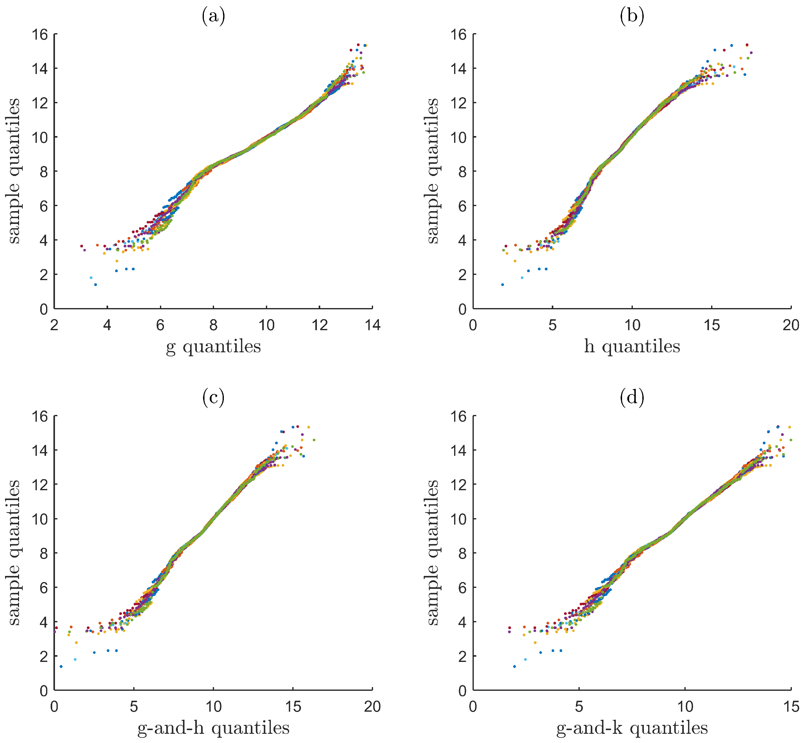
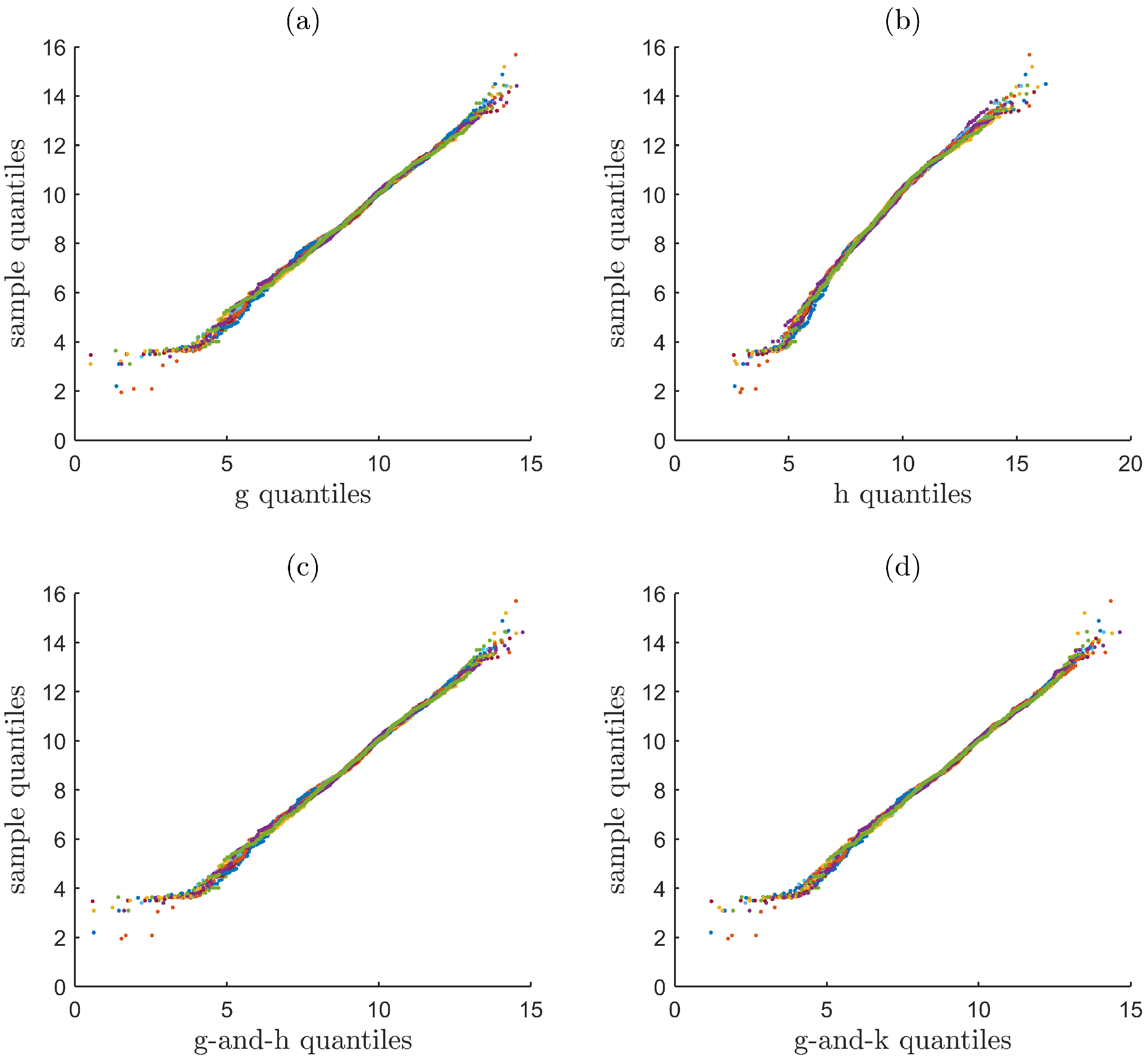
As an example, Figure 1 and Figure 2 show the Q-Q plots of the sample quantiles plotted against the quantiles of the models that are fitted to the monthly blocks of 1998 and 2003, respectively. In each panel (a, b ,c, or d), twelve Q-Q plots are shown, corresponding to the monthly blocks of a year. For year 1998, the g distribution (a) is unable to adequately model both tails of the data, as the data suggests a heavier-tailed distribution than the g distribution. The h distribution (b) also shows a lack of fit for both tails, primarily due to its inability to account for the asymmetry in the data. The g-and-h and g-and-k distributions (c and d) appear to be adequate for the right tail while showing a better fit for the left tail, as they are able to model both the asymmetry and the heavy tails. For year 2003, the fact that the g distribution fits most of the data well and that the h distribution fails to do so indicates that the primary feature of the data is asymmetry rather than possessing heavy tails. All of the models except for the h distribution are able to adequately describe most part of the data. Notice that for both years, all of the models struggle to fit the far left tail of the data. The data suggests that a distribution whose far left tail is lighter than that of our models is appropriate.

From studying the individual Q-Q plots, we know that it is important to model both the asymmetry and the heavy tails, and that the parameters may not be constant over time. Next, we study how the parameters of the g-and-h and g-and-k distributions evolve over the years. To achieve this, we construct a time series plot (against the years $\left\{t\right\}$) of each parameter estimate for each month s. 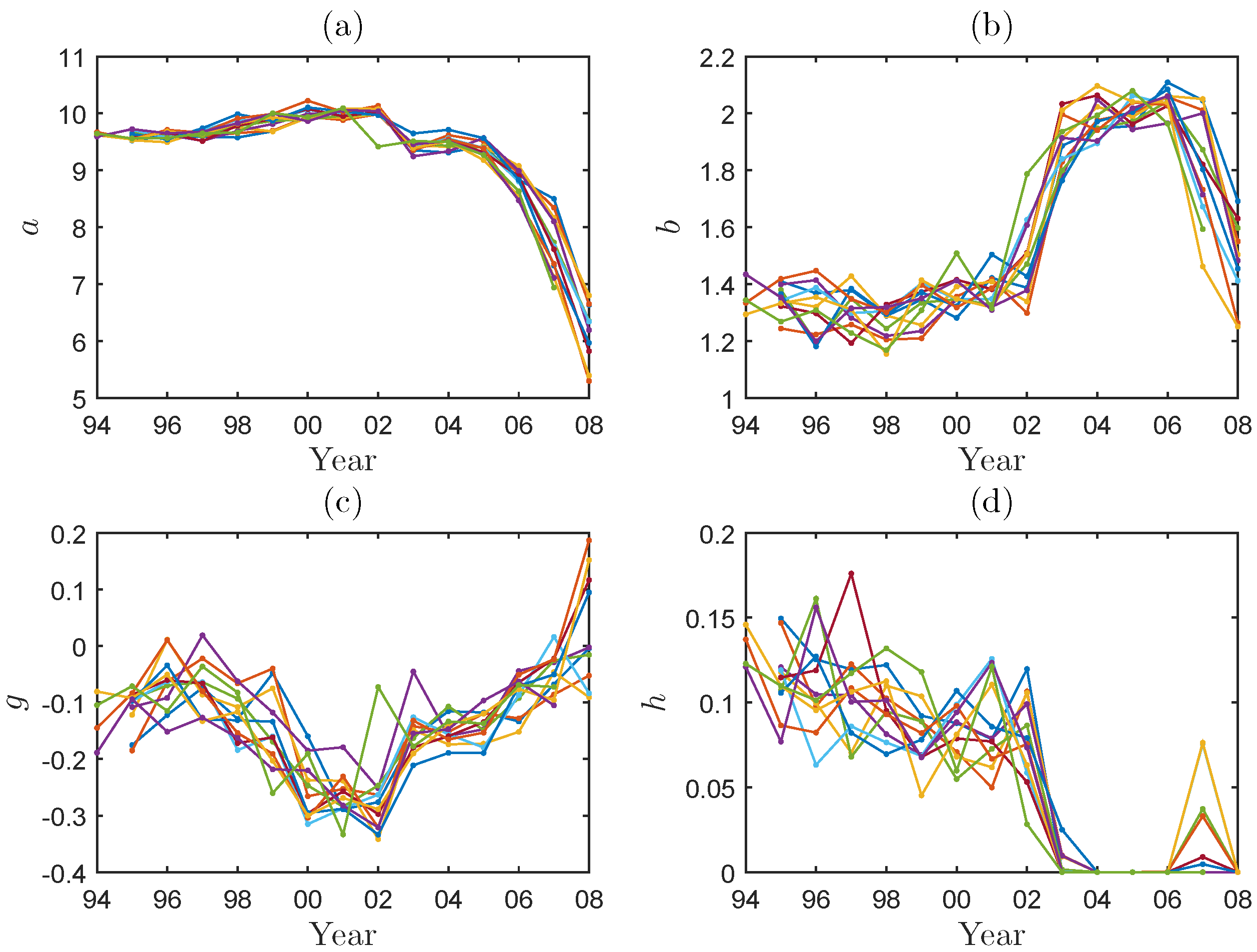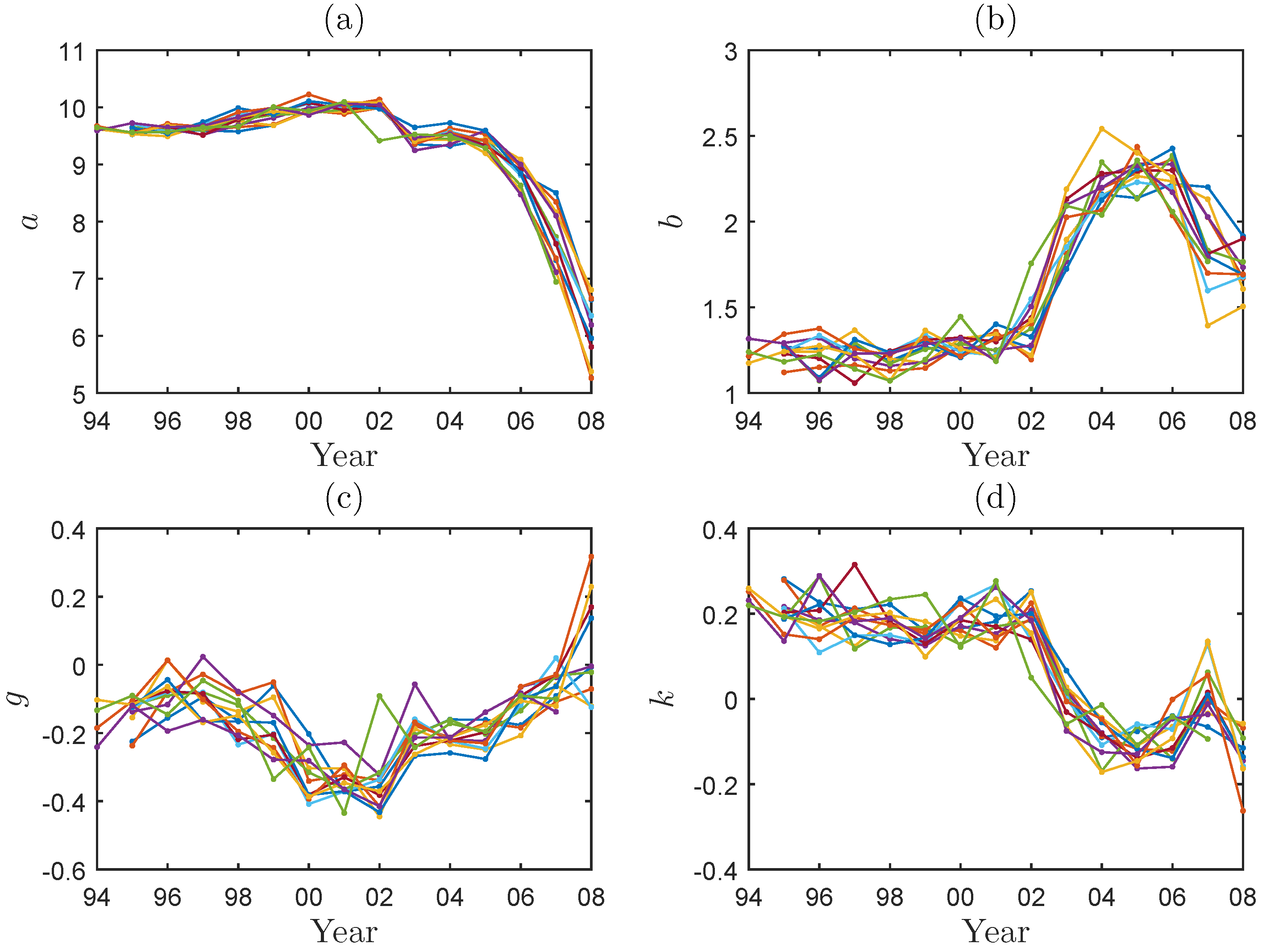Such time series plots are shown in Figure 3 and Figure 4 for the g-and-h and the g-and-k models, receptively. For a given parameter, there are twelve observations plotted for each year, corresponding to the calendar months, except for 1994 and 2008. The missing observations in those years is due to the fact that our dataset starts in September and ends in November and that we have excluded November, 2008 from the study as there are only 37 claims in that month.

Some interesting observations can be made by examining these time series plots. It is clear from the plots that the parameters vary significantly over the years for both models. The underlying process of each parameter appears to be non-stationary. The scale parameters are negatively correlated with the tail-shape parameters; the location parameters are negatively correlated with the asymmetry parameters. It seems that there is a structural change in year 2002, where the severity distribution starts to increase in scale but become less heavy-tailed; the location of the distribution starts to shift downward while the skewness starts to move from negative to neutral or even positive. In fact, the g-and-k model reveals (in panel (d) of Figure 4) that the severity distribution switches gradually from being heavy-tailed to being light-tailed (relative to the normal distribution) after 2002.

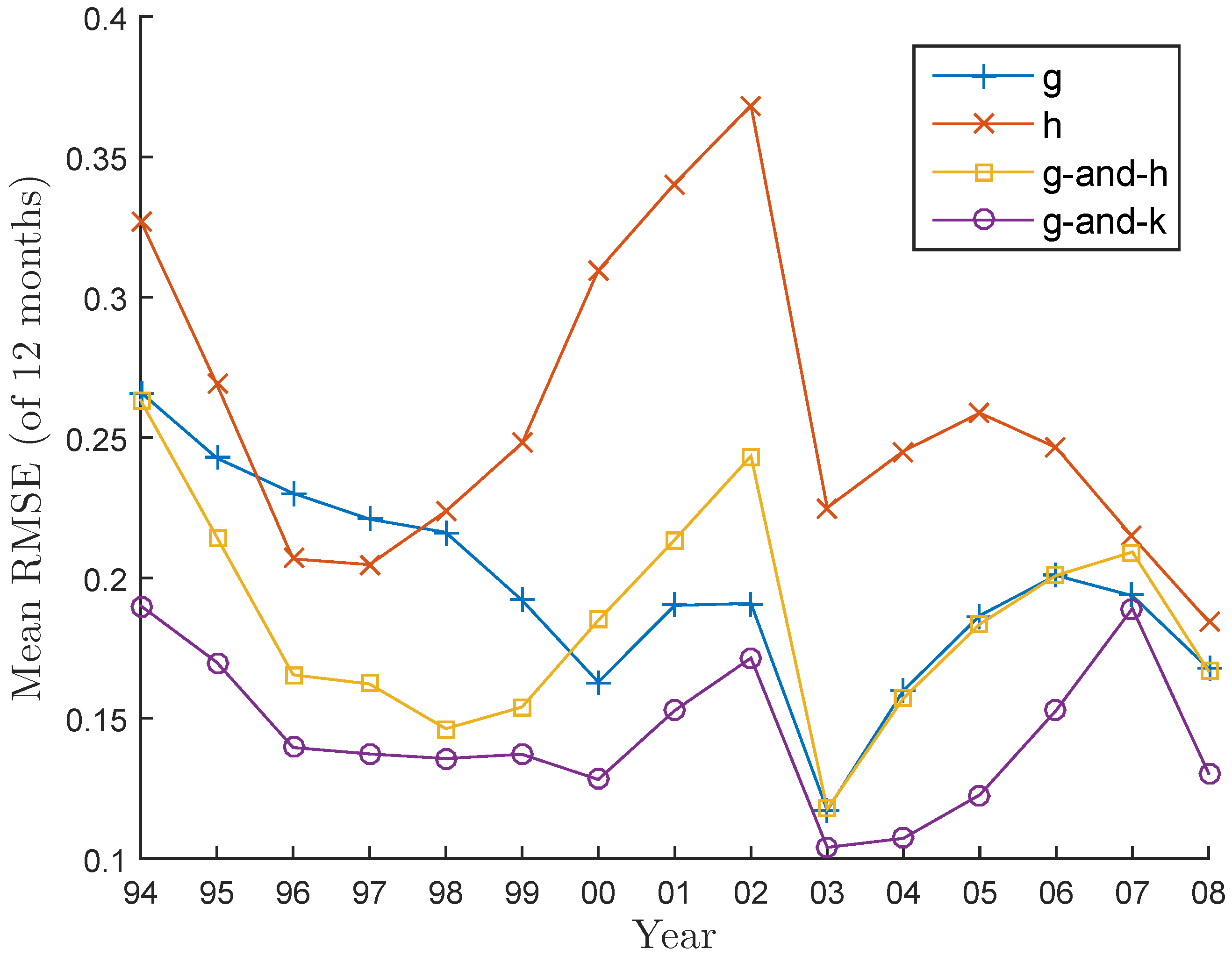
To compare the goodness-of-fit between the models for each year, we compute RMSE using Equation (122) for each monthly block and then plot the mean of the twelve monthly RMSE values for each year. The result is a time series plot of the average RMSE values for each model, shown in Figure 5. We can see that the goodness-of-fit varies both over time and across the models. It is interesting to see that the g-and-k distribution clearly provides the best fit in every year and that the h distribution is worst for most of the years.

8. Conclusions

In this paper we have proposed a new family of claims reserving models for non-life insurance severity modelling corresponding to a flexible class of Tukey elongation transform models. We have outlined the characterization of the sub-families of g, h, k, j, h-h, g-and-h, g-and-k, g-and-j and generalised g variants. Furthermore, we have studied the properties of such models, including deriving novel relationships for the tail behaviour and the population L-moments for such models. Furthermore, we have demonstrated the estimation of these claim model parameters can be performed using the method of L-moment, which can often be more accurate and efficient than alternative procedures based on moment-matching or maximum likelihood. Finally, we have applied the methods and models to calibration of claim severity models for a large insurance database based on CTP automotive claims data from Australia.