Using Climate and Weather Data to Support Regional Vulnerability Screening Assessments of Transportation Infrastructure

Abstract

Extreme weather and climate change can have a significant impact on all types of infrastructure and assets, regardless of location, with the potential for human casualties, physical damage to assets, disruption of operations, economic and community distress, and environmental degradation. This paper describes a methodology for using extreme weather and climate data to identify climate-related risks and to quantify the potential impact of extreme weather events on certain types of transportation infrastructure as part of a vulnerability screening assessment. This screening assessment can be especially useful when a large number of assets or large geographical areas are being studied, with the results enabling planners and asset managers to undertake a more detailed assessment of vulnerability on a more targeted number of assets or locations. The methodology combines climate, weather, and impact data to identify vulnerabilities to a range of weather and climate related risks over a multi-decadal planning period. The paper applies the methodology to perform an extreme weather and climate change vulnerability screening assessment on transportation infrastructure assets for the State of Tennessee. This paper represents the results of one of the first efforts at spatial vulnerability assessments of transportation infrastructure and provides important insights for any organization considering the impact of climate and weather events on transportation or other critical infrastructure systems.

1. Introduction

Growing attention is being devoted to improving our understanding of the vulnerability of critical infrastructure to extreme weather events and climate change (Pollard, 2015 [1]; Schulz, 2007 [2]). In the case of transportation, extreme weather can physically damage infrastructure and disrupt travel mobility, resulting in public health, economic, social and ecological impacts whose consequences can seriously threaten the viability of individual communities or entire regions (Savonis et al., 2008 [3]; TRB, 2008 [4])). Because a functional infrastructure system involves an integrated and substantial network of different components across a widespread area, many organizations are taking a regional perspective when assessing extreme weather and climate vulnerability. Regional approaches face significant challenges, however, because most regions are characterized by a varying topography that leads to diverse climate conditions, various forms of extreme weather, and differing stressors and impacts on infrastructure.

Given this nascent field and the challenges in assessing impacts from climate change in localized areas, in 2014, the Transportation Research Board (TRB) issued a practitioner’s guide and report aimed at assisting state Departments of Transportation (DOTs) incorporate climate change and extreme weather adaptation measures to the highway system in planning efforts, which included a multi-step framework for undertaking an adaptation assessment (TRB NCHRP, 2014 [5]). Obtaining climate data and assessing vulnerabilities were two steps in this framework, but the report noted that as recently as 2014 “the research team could find no state transportation agency that has undertaken all of the steps of the diagnostic framework—or for that matter adaptation planning in general (at least in an organized and systematic way)” (TRB NCHRP, 2014, p. 14 [5]).

To begin to address this problem in the transportation context, the U.S. Department of Transportation, Federal Highway Administration (FHWA) funded a pilot program involving five state DOTs or Metropolitan Planning Organizations (MPOs) from 2010 to 2011 to test a conceptual model for conducting climate change vulnerability assessments (FHWA, 2016 [6]). This work culminated in a refinement of the model and the publication of a Climate Change and Extreme Weather Vulnerability Assessment Framework that another 19 state DOTs and MPOs were selected to implement in a pilot study (FHWA, 2012 [7]). Tennessee was one state selected and serves as the case study for application of the methodology presented in this paper.

Defining and assessing vulnerability in a variety of contexts not solely related to climate change has been studied extensively in the transportation context. Recent efforts have focused on methods and criteria for identifying vulnerable links at the network level (Knoop, 2012 [8]; Taylor 2007 [9]; Erath, 2010 [10]), for estimating the impacts of road or link closures within networks (Jenelius, 2007 [11]; Knoop, 2008 [12]), understanding vulnerability in the context of socio-economic impacts from a loss of critical transportation assets within a network (Taylor, 2006 [13]), and defining vulnerability in the context of vulnerability assessments for specific systems, such as maritime transportation (Berle, 2011 [14]). Jenelius et al. have noted that the term “vulnerability” has multiple definitions and the meaning may depend on the context and goals of the study (Jenelius, 2006 [15]).

Much of FHWA’s work to develop a vulnerability assessment framework emanated from a major study to understand climate risk at coastal ports in the Gulf of Mexico, with a focus on Mobile, Alabama (known as the Gulf Coast Studies) (FHWA 2016 [16]). In 2015, FHWA published the Mobile, Alabama case study implementing the framework for evaluating the vulnerability of transportation assets to climate change stressors (FHWA, 2015 [17]). In these studies, FHWA defined vulnerability as a function of three indicators: (1) exposure to climate events, such as sea level or temperature rise; (2) the sensitivity of the asset or system when it is exposed to the climate impact; and (3) the adaptive capacity of the system or asset (e.g., the ability to cope or adjust in response to an impact) (FHWA, 2015 [17]). This definition and approach to vulnerability analyses with a focus on exposure, sensitivity, and adaptive capacity is consistent with the treatment of vulnerability in the literature, especially in the context of climate change (Smit and Wandel, 2006 [18]; Kelley & Adger, 2000 [19]; Xenairos, et al., 2016 [20]; Füssel, 2009 [21]; IPCC, 2007 [22]).

The screening tool set forth in this paper builds on the FHWA’s vulnerability concepts with a definition of vulnerability appropriate for use in a screening assessment. Using climate data and impact analysis, we define the term “vulnerability” to be a function of the historic frequency of an extreme weather event or climate condition, the projected change in those frequencies or conditions over the forecast period, and the potential impact of those events or conditions on selected assets or areas. Using this methodology, we derived future vulnerability scores where the data was sufficient to reasonably extrapolate potential future conditions; and where the data was not sufficient to project future conditions, we calculated current vulnerability scores. Accordingly, the “vulnerability” identified through this screening assessment does not take into consideration specific characteristics of a single asset or location that may make the asset more or less vulnerable; rather, the approach and methods are beneficial for screening a broad range of assets and locations to determine what types or categories of assets in particular areas may be more or less vulnerable to climate change and certain types of extreme weather events. This vulnerability screening assessment then enables planners and asset managers to more efficiently target scarce resources on assets or areas of most concern, and to conduct a more detailed vulnerability assessment (one that can take into account the sensitivities of individual assets) on a subset of selected assets.

As recognized in both TRB’s and FHWA’s work, one of the first steps in any effort to inform climate change adaptation and planning is a vulnerability assessment aimed at identifying where assets or communities may be most at risk in a changing world. However, obtaining and using climate and weather data in a meaningful way at localized scales to support vulnerability assessments has been a significant challenge to many planners and policy makers attempting to better understand the vulnerabilities of their infrastructure (transportation or otherwise) and direct limited resources (USAID, 2014 [23]). Accordingly, this paper focuses on the development of a methodology to assess future extreme weather events and climate conditions to which critical infrastructure may be exposed, to quantify the severity of impacts from extreme weather events, and to combine this information in order to identify vulnerabilities to transportation systems over multi-decadal planning periods.

The methods regarding climate and weather data discussed in this paper were applied to a set of transportation assets that were determined to be “critical” assets in the State of Tennessee using an approach described by Abkowitz, et al., 2016 [24]. Assets were determined to be “critical” if they met certain performance criteria (such as average daily traffic, volume of freight, or alternative route availability), were important to the functioning of a regional network, or were identified through a multi-stakeholder input process. This approach to defining critical assets was appropriate for the statewide breadth of the study, but also remained in keeping with the literature on criticality (Knoop, et al., 2012 [8]; Taylor, 2007 [9]; Jenelius, 2006 [15]; Kim & Lee, 2006 [25]; Schulz, 2007 [2]). The selection of assets to which the vulnerability screening assessment can be applied will vary depending on the planning context and goals.

Climate change vulnerability assessments are an emerging practice, so new that there “is as yet no consensus on what constitutes “best practices” in spatial (vulnerability assessments)” (USAID, 2014 [23]; Mitsakis, et al., 2013 [26]). This paper represents the results of one of the first efforts at spatial vulnerability assessments of transportation infrastructure and provides important insights for organizations considering the impact of climate and weather events. Although the methods discussed here are illustrated using the State of Tennessee as a case study, they are applicable beyond the region and beyond the transportation sector to any assets that could be impacted by extreme weather or climate change. Application of the methods to other areas (such as low income areas) warrants further exploration.

2. Materials and Methods

2.1. Obtaining and Understanding Extreme Weather and Climate Data for Use in Vulnerability Assessments

The American Society of Civil Engineers (ASCE) has recognized that designing long-lived infrastructure today presents a significant problem when there is substantial uncertainty regarding the weather and climate to which that infrastructure will be exposed in the future (ASCE, 2015 [27]). Applying engineering and design standards that were created for a climate that may not be relevant for a substantial portion of the design life of a piece of infrastructure presents particular challenges. (Meyer, 2006 [28]). Notably, there is an important difference between climate and weather. Weather is generally difficult to predict very far in advance and is subject to rapid changes. Climate, in contrast, is more predictable because it represents a type of averaging of weather events over longer time periods. In short, “weather is chaotic, but climate generally is not” (Archer, 2011 [29]).

Most transportation vulnerability assessments to date have been performed in coastal areas and have focused on storm surge and sea level rise (FHWA, 2009 [30]; FHWA, 2015 [17]), events that are not a concern for inland states such as Tennessee. In contrast, thunderstorms and rockslides represent some of the most significant threats to transportation assets in Tennessee and other mountainous inland areas. The wind, rain, and hail of a specific thunderstorm are discrete weather events, whereas overall precipitation an area can expect over a period of time is generally considered a climate variable, and is arguably the single largest predictor of the occurrence of rockslides (Chernicoff, 2007 [31]). Many modeling tools have been developed to assist with projections of sea level rise (NOAA, 2015 [32]), yet few exist to project specific storm or extreme weather events with reasonable accuracy or at reasonable cost (TRB NCHRP, 2014 [5]). Even with respect to climate, uncertainty in the global climate models increases as one reduces the geographic scale to regional and local areas, and these uncertainties are only compounded when attempting to project extreme weather events (ASCE, 2015 [27]).

Global climate models (GCMs) divide the world into large grid cells that are typically 100–300 km squares. This coarse resolution is less useful for regional or local planners and policy makers who need to make decisions and estimate impacts on much smaller scales (Wall, et al., 2014 [33]). Climate at the regional level is also impacted by local topography (such as mountains or lakes) that are not well accounted for in the GCMs. A technique known as “downscaling” provides this finer resolution data from the coarser global climate models that is more useful at a local or regional scale.

There are two types of downscaling, statistical and dynamical. Dynamical downscaling combines the conditions specified by a GCM with high resolution regional climate models (RCMs) which can often include observed data to produce much finer resolution data, often at grid sizes of 20–60 km. Statistical downscaling uses regression analyses that are designed to link the climate drivers of the GCMs with local climates, and can be quite complex (Climate Decisions, 2008 [34]). Statistical downscaling can be beneficial because a number of model outputs, rather than just one, are utilized, correcting for biases that may be present in any one model. Statistical downscaling also does not take the tremendous computing power that is required of dynamical downscaling, and is therefore frequently used in research, including both sources of the CMIP data utilized in this paper. However, one limitation with statistical downscaling is that it assumes a certain statistical relationship between the global climate drivers and local climate conditions; if that relationship shifts because of climate change, the projections may not be accurate (IPCC, 2013 [35]).

Projecting future extreme weather events presents additional uncertainties, primarily because of non-stationarity present in weather and climate data. However, there is much ongoing work in this field, and the application of non-stationary generalized extreme value (GEV) distribution can be used to allow a climate model to vary certain parameters over time. Condon has used this approach to estimate future flood risk for the Upper Truckee River Basin (Condon, et al., 2015 [36]). In the context of a network-level risk analysis, Wall et al. have applied GEV distribution to obtain insight into future exposure of drainage infrastructure (culverts) to extreme precipitation events in Washington State (Wall, et al., 2014 [33]).

Similarly, although historic extreme weather data can more easily be obtained at localized scales and is independent of model uncertainties, the data can be limited, and may vary over time in response to population shifts, improved weather monitoring technologies, and recordkeeping methods. Projecting future events based on trends of past weather events can be useful, but must be predicated on an understanding of the limits of this data (FHWA, 2011 [37]). Nevertheless, TRB has suggested including a focus on areas “where experience with extreme weather suggests future problems will exist...” (TRB, NCHRP, 2014, p. 15 [5]). As discussed below, historic extreme weather data is used in the developed methodology to allow planners to quickly assess where extreme weather has been a problem in the past, and can provide insight into areas where future problems may continue. Moreover, the methodology presented is meant to be useful to planners now, despite the continued uncertainly, especially with respect to changes in frequency or severity of extreme weather events. This methodology can be augmented and refined as developments in the climate science allow for increased certainty with respect to projections of changes in extreme weather events.

Working within the limitations of available historical extreme weather data and climate projections, the Tennessee project developed a screening tool, easily transferable to other applications, for identifying where transportation infrastructure might be most vulnerable to extreme weather in the future. This screening-level assessment can identify assets or areas where it may be advisable to focus limited resources for a more comprehensive assessment using existing TRB or FHWA frameworks for assessing vulnerability or undertaking adaptation initiatives (TRB NHCRP, 2014 [5]; FHWA, 2015 [17]). Most transportation vulnerability assessments have primarily utilized climate projections to try to understand changes in climate and the potential for extreme weather (Washington State Department of Transportation, 2011 [38]; TRB NCHRP, 2014 [5]). Notably, the Tennessee project went further, and included historic data on specific extreme weather events, as well as historic climate data where it was available and where it could reasonably provide for inferences about future exposure. This hybridized approach provides a better understanding of both climate projections in the region and the range of plausible extreme weather events, as well as insight into how these two considerations might interact in the future. Thus, both historic weather and climate data, as well as future climate projections, were crucial to the study.

2.2. Data for Historic Extreme Weather Events

The National Weather Service (NWS) has long been interested in tracking extreme weather events, beginning in the 1950s with the establishment of an information system to define extreme weather and to characterize such occurrences in the U.S. (NWS, 2007 [39]). Referred to as the Storm Events Database (NOAA, 2015 [40]), it contains the records of storms and other weather phenomena having sufficient intensity to cause loss of life, injuries, significant property damage, and/or disruption to commerce. Indeed, the NWS is the primary and only source of long term records that exist of domestic flood damages (Downton, 2005 [41]).

The Storm Events Database establishes certain thresholds of impact and weather characteristics (such as wind speed, inches of ice, etc.) that must be present in order for the event to meet a particular definition of extreme weather. The Storm Events Database also includes entries for other important meteorological events, such as record maximum or minimum temperatures, or precipitation that occurs in connection with another event.

The database contains records beginning in January 1950, catalogued according to the county where the extreme weather event was observed. Changes have occurred in the data collection protocol over time as new event types have been added and more sophisticated weather monitoring and recording methods evolved. Beginning in 1950 through 1954, only tornado events were recorded. From 1955 through 1995, in addition to tornadoes, thunderstorm wind and hail events were also included. Since 1996, 45 additional extreme weather event types have been added, bringing the total number of event types to 48. As new extreme weather event types have been included, attributes describing geographic location, event impacts, and other event specific information have remained consistent. For analysis purposes, this provides an opportunity to perform comparisons between event types over space and time, subject to normalizing the frequency of occurrence by the number of years for which the particular event type has been recorded.

One notable caveat is the intensity threshold that NWS uses for an event to be considered for database inclusion (i.e., loss of life, injuries, significant property damage, crop damage, and/or disruption to commerce). The use of a threshold based on damages implies that extreme weather events with similar characteristics are more likely to meet the intensity threshold in densely populated areas where more people and infrastructure are potentially exposed. This may result in a larger number of observations in the database from urbanized areas in comparison to rural areas. This damage and loss bias towards areas with higher wealth and population is well understood (Gall, et al., 2009 [42]).

As noted earlier, downscaled climate forecast models have been developed for projecting future temperature and precipitation conditions. However, performing a similar exercise involving other forms of extreme weather that may be particularly disastrous to certain infrastructure or assets, such as high speed winds, is more challenging. More recently, available climate data does contain variables related to surface wind speed, but these data are only beginning to be explored to identify trends in wind speed resulting from climate change (Kulkarni, 2014 [43]), and have not been downscaled sufficiently to support a project focused on a single state such as Tennessee. Accordingly, the NWS Storm Events Database was an important source of data to increase the utility of the study’s analysis and results.

2.3. Projected Climate Data from Climate Modeling

A statewide vulnerability assessment presents unique challenges in projecting future climate conditions involving temperature and precipitation. Although researchers are actively engaged in developing climate models to aid this process, making such projections involves an understanding of many complex weather and climate related variables and interactions. As a result, the confidence one can have in the predictive results diminishes when downscaling global climate models from a regional to a more local level (ASCE, 2015 [27]).

The TRB NCHRP report identified a variety of sources for climate projection data, noting that some are difficult to obtain, complex, or expensive (TRB NCHRP, 2014) [5]. In keeping with the study’s scope, we sought climate data that was reputable with respect to accuracy and could easily be obtained and utilized by planners with limited resources. Of particular interest was the work of the World Climate Research Programme (WCRP, 2015 [44]), which established the Coupled Model Intercomparison Project (CMIP) to develop climate models and improve the accuracy of their projections. CMIP has proceeded in four sequential phases, CMIP1 through CMIP5 (there is no CMIP4), involving various methods of data collection, analysis, simulations, control runs, and input variability. CMIP data comes from virtually every global climate modeling group in the world and are used to inform the formal reports of the Intergovernmental Panel on Climate Change (IPCC), the leading international organization for assessing climate change established by the United Nations Environmental Programme and the World Meteorological Organization.

We relied on two sources of climate data for this study, statistically downscaled monthly averages of CMIP3 data by county and statistically downscaled daily values of CMIP5 data by 12 km × 12 km grid cell. Both of these sources of climate data ultimately come from raw 1/8 degree downscaled CMIP climate projection data (WCRP, 2015 [44]). CMIP5 climate projections are recognized as the state of the art and most advanced projections available. However, because at the time of the study much research around the world had been initiated with CMIP3 data and it has been well tested the FHWA has recommended that CMIP5 data not be used to replace CMIP3 data, but rather to supplement it (FHWA, 2014 [45]). Accordingly, the Tennessee study made use of CMIP3 data to generate vulnerability scores and used CMIP5 data to validate the results of climate analyses for the state’s most populous areas and to provide additional, more refined climate information for those areas.

The CMIP3 data utilized in this study was compiled by researchers at the University of Georgia, who generated statistically downscaled monthly averages of both precipitation and temperature for every county in the Southeastern United States for each year through 2060 (Maurer, 2007 [46]). Given the statewide scope of the Tennessee study, the project focused on the Tennessee data generated by the University of Georgia work, which provided monthly, county-level projected climate data through the year 2060. These county-level data can be particularly useful to planners attempting to project climate variables across areas too large to make the FHWA tool practical. (The State of Tennessee covers 109,247 square kilometers, which would require over 9000 grids to be separately selected and analyzed, and would result in a minimum of approximately 2275 sets of data output to be analyzed, assuming four grid cells are analyzed together.) Accordingly, the CMIP3 data was the primary source of climate projections used in our study, and was incorporated into the spatial analysis of trends and the final vulnerability scores.

While downscaled CMIP climate projections represent some of the best science available, the data can be cumbersome to access and analyze. Accordingly, as part of its Climate Change Vulnerability Assessment Framework, FHWA published a CMIP Climate Data Processing Tool (ICF, 2015 [47]). The tool consists of an Excel spreadsheet that processes raw CMIP data into information that is easily understandable. Although it was developed with transportation planners in mind, the outputs would be useful to any assessment of the impacts of climate and weather on a broad range of assets. The tool allows users to apply downscaled CMIP3 or CMIP5 data to analyze a small geographical area (i.e., a maximum of four, 12 km × 12 km grid cells) for projected precipitation and temperature values. While the FHWA tool greatly improves the accessibility of climate data for practitioners, the small spatial extent of the output from the FHWA climate data processing tool made its application to the entire state of Tennessee impractical. Therefore, for this study we utilized the tool only to obtain CMIP5 climate projections for the major cities in the state.

2.4. Assessing Historic Extreme Weather Event Frequency and Trends

An assessment of historic extreme weather events in Tennessee was conducted to generate annual frequencies by county for each type of extreme weather event. These frequencies provide a baseline for profiling the extent to which Tennessee is exposed to extreme weather according to location and specific event types. Because the ultimate goal of this work is to understand what might occur over a 25-year planning horizon, this information needs to be considered in concert with what might be anticipated in the future. Therefore, the study evaluated trends in event frequencies.

Since the inception of the NWS Storm Events Database, 23 of the 48 extreme weather event types have been observed in Tennessee with some degree of regularity. These event types are listed in

Table 1. Tennessee Historical Extreme Weather Event Types.

Cold/Wind Chill	Frost Freeze	Lightning
Drought	Funnel cloud	Sleet
Dust devil	Hail	Strong wind
Excessive heat	Heat	Thunderstorm wind
Extreme cold/wind chill	Heavy rain	Tornado
Flash flood	Heavy snow	Winter storm
Flood	High wind	Winter weather
Freezing fog	Ice storm	-

, with their corresponding definitions provided in

Table 2. Extreme Weather Event Categories.

Weather Event Category	NWS Event Type(s) Included	NWS Extreme Weather Event Definition
Cold	Cold/wind chill	Period of low temperatures or wind chill temperatures reaching or exceeding locally/regionally defined advisory (typical value is −18° F or colder) conditions, on a widespread or localized basis. There can be situations where advisory criteria are not met, but the combination of seasonably cold temperatures and low wind chill values (roughly 15° F below normal) must result in a fatality. In these situations, a cold/wind chill event may be documented if the weather conditions were the primary cause of death as determined by a medical examiner or coroner. Normally, cold/wind chill conditions should cause human and/or economic impact. This event is only used if a fatality/injury does not occur during a Winter Precipitation event
	Extreme cold/wind chill	A period of extremely low temperatures or wind chill temperatures reaching or exceeding locally/regionally defined warning criteria (typical value around −35° F or colder), on a widespread or localized basis. Normally these conditions should cause significant human and/or economic impact. However, if fatalities occur with cold temperatures/wind chills but extreme cold/wind chill criteria are not met, the event is recorded in the database as a Cold/Wind Chill event. This event is only used if a fatality/injury does not occur during a Winter Precipitation event.
Hot	Heat	A period of heat resulting from the combination of high temperatures (above normal) and relative humidity. A Heat event occurs and is recorded whenever heat index values meet or exceed locally/regionally established advisory thresholds. Fatalities or major impacts on human health occurring when ambient weather conditions meet heat advisory criteria are reported using the Heat category. If the ambient weather conditions are below heat advisory criteria, a Heat event entry is permissible only if a directly-related fatality occurred due to unseasonably warm weather, and not man-made environments.
	Excessive heat	This results from a combination of high temperatures (well above normal) and high humidity. An Excessive Heat event is reported in the database whenever heat index values meet or exceed locally/regionally established excessive heat warning thresholds, on a widespread or localized basis. Fatalities (directly-related) or major impacts to human health occurring during excessive heat warning conditions are reported using this event category. Fatalities or impacts to human health occurring when conditions meet locally/regionally defined heat advisory criteria are reported within the Heat event category instead.
Wind	Strong wind	Non-convective winds gusting less than 50 knots (58 mph), or sustained winds less than 35 knots (40 mph), resulting in a fatality, injury, or damage. Inland counties which experience strong winds/damage associated with tropical cyclones are recorded under the Tropical Depression or Tropical Storm category, as appropriate, rather than as a Strong Wind event.
	High wind	Sustained non-convective winds of 35 knots (40 mph) or greater lasting for one hour or longer or winds (sustained or gusts) of 50 knots (58 mph) for any duration (or otherwise locally/regionally defined), on a widespread or localized basis. In some mountainous areas, the above numerical values are 43 knots (50 mph) and 65 knots (75 mph), respectively. The High Wind event name is not used for severe local storms, tropical cyclones, or winter storm events. Events with winds less than the High Wind event threshold numbers, resulting in fatalities, injuries, or significant property damage, are encoded as a Strong Wind event.
	Thunderstorm wind	Winds arising from convection (occurring within 30 min of lightning being observed or detected), with speeds of at least 50 knots (58 mph), or winds of any speed (non-severe thunderstorm winds below 50 knots) producing a fatality, injury, or damage. Maximum sustained winds or wind gusts (measured or estimated) equal to or greater than 50 knots (58 mph) are always entered. Events with maximum sustained winds or wind gusts less than 50 knots (58 mph) are entered only if they result in fatalities, injuries, or serious property damage.
Twister	Funnel cloud	A rotating, visible extension of a cloud pendant from a convective cloud with circulation not reaching the ground. This would include cold-air funnels which typically form in a shallow, cool air mass behind a cold front. The funnel cloud should be large, noteworthy, or create strong public interest to be included in the database.
	Dust devil	A ground-based, rotating column of air, not in contact with a cloud base, usually of short duration, rendered visible by dust, sand, or other debris picked up from the ground, resulting in a fatality, injury, or damage. Dust devils usually result from intense, localized heating interacting with the micro-scale wind field. Dust devils that do not produce a fatality, injury, or significant damage are also entered as an event if they are unusually large, noteworthy, or create strong public interest
	Tornado	A violently rotating column of air, extending to or from a cumuliform cloud or underneath a cumuliform cloud, to the ground, and often (but not always) visible as a condensation funnel. In order for a vortex to be classified as a tornado, it must be in contact with the ground and extend to/from the cloud base, and there should be some semblance of ground-based visual effects such as dust/dirt rotational markings/swirls, or structural or vegetative damage or disturbance. An Enhanced Fujita (EF) or Fujita (F) Damage Scale value is entered, depending on the year of occurrence.
Hydrologic	Heavy rain	An unusually large amount of rain which does not cause a Flash Flood or Flood, but causes damage or other human/economic impact. Heavy rain situations, resulting in urban and/or small stream flooding, are classified as a Heavy Rain event or another suitable event that occurred at the same time.
	Flash flood	A rapid and extreme flow of high water into a normally dry area, or a rapid water level rise in a stream or creek above a predetermined flood level, beginning within six hours of the causative event (e.g., intense rainfall, dam failure, ice jam-related), on a widespread or localized basis. Ongoing flooding can intensify to flash flooding in cases where intense rainfall results in a rapid surge of rising flood waters.
	Flood	Any high flow, overflow, or inundation by water which causes or threatens damage. In general, this would mean the inundation of a normally dry area caused by an increased water level in an established watercourse, or ponding of water, generally occurring more than six hours after the causative event, and posing a threat to life or property. This can be on a widespread or localized basis. River flooding may be included in the Flood category. However, such entries should be confined only to the effects of the river flooding, such as roads and bridges washed out, homes and businesses damaged, and the dollar estimates of such damage
Lightning	Lightning	A sudden electrical discharge from a thunderstorm, resulting in a fatality, injury, and/or damage directly related to the lightning strike. Anyone seeking or receiving medical attention following a lightning incident is counted as a lightning injury. Anyone reporting numbness, a tingling sensation, a headache, or other pain following a lightning incident, whether or not they receive treatment, is also counted as an injury.
Hail	Hail	Frozen precipitation in the form of balls or irregular lumps of ice. Hail 3/4 of an inch or larger in diameter will be entered. Hail accumulations of smaller size which cause property and/or crop damage, or casualties, are also recorded.
Drought	Drought	A deficiency of moisture that results in adverse impacts on people, animals, or vegetation over a sizeable area. Conceptually, drought is a protracted period of deficient precipitation resulting in extensive damage to crops, resulting in loss of yield. There are different kinds of drought: meteorological, agricultural, hydrological, and social-economic. Droughts are rated as D0, D1, D2, D3, or D4 based on the intensity of the moisture deficiency and other factors. A drought event is included in the database when the drought is rated as a D2 classification, or higher.
Winter	Winter weather	A winter precipitation event that causes a death, injury, or a significant impact to commerce or transportation but does not meet locally/regionally defined warning criteria. A Winter Weather event could result from one or more winter precipitation types (snow, or blowing/drifting snow, or freezing rain/drizzle), on a widespread or localized basis.
	Sleet	Sleet accumulations meeting or exceeding locally/regionally defined warning criteria (typical value is ½ inch or more).
	Freezing fog	Fog which freezes on contact with exposed objects and forms a coating of rime and/or glaze, on a widespread or localized basis, resulting in an impact on transportation, commerce, or individuals. Freezing fog can occur with any visibility of six miles or less. Even small accumulations of ice can have an impact.
	Frost/Freeze	A surface air temperature of 32 °F or lower, or the formation of ice crystals on the ground or other surfaces, over a widespread or localized area for a period of time long enough to cause human or economic impact.
	Heavy snow	Snow accumulation meeting or exceeding locally/regionally defined 12 and/or 24 h warning criteria, on a widespread or localized basis. This could mean such values as 4, 6, or 8 inches or more in 12 h or less; or 6, 8, or 10 inches in 24 h or less. In some heavy snow events, structural damage, due to the excessive weight of snow accumulations, may occur in the few days following the meteorological end of the event.
	Winter storm	A winter weather event which has more than one significant hazard (i.e., heavy snow and blowing snow; snow and ice; snow and sleet; sleet and ice; or snow, sleet and ice) and meets or exceeds locally/regionally defined 12 and/or 24 h warning criteria for at least one of the precipitation elements, on a widespread or localized basis. Normally, a Winter Storm would pose a threat to life or property.
	Ice storm	Ice accretion meeting or exceeding locally/regionally defined warning criteria (typical value is 1/4 or 1/2 inch or more), on a widespread or localized basis. This event is also recorded for a fatality/injury that results from hypothermia in a power loss situation due to an ice storm.

. (Tropical depressions, tropical storms and wildfires have also been observed in Tennessee, but so rarely recorded in the Storm Events Database that these event types were removed from consideration.) Collectively, there have been over 27,000 recorded events in the state since the Storm Events Database was established (NOAA, 2015 [40]).

From an analytical perspective, it is important to note that many of these event types categorized by NWS do not represent discrete, stand-alone weather conditions, but rather gradations of the severity of certain weather forms. For example, “excessive cold/wind chill” represents conditions that are more severe than “cold/wind chill”. Another example is the relationship between “funnel cloud”, “dust devil”, and “tornado”, all of which are characterized by circular wind rotation. Because of these relationships, and to reduce event types to a more manageable number for analysis, the aforementioned 23 event types were aggregated into nine extreme weather event categories. The weather event category, the NWS events contained within those categories, and the specific definition of those NWS extreme weather events are displayed in Table 2.

For each of the nine extreme weather event categories, the average annual number of recorded events was compiled for each of the state’s 95 counties. Figure 1 shows an example of one of these calculations—for wind events—by county (see Figure 1). Displaying the data in this way quickly conveys that counties with major urban areas experience higher frequencies of damage-inducing extreme wind events (Figure 1). Analysis of the frequency of different wind event types indicates that straight-line winds and wind funnels have been a frequent occurrence in Tennessee. Considering the particularly destructive nature of these wind events to the transportation system, understanding the current frequencies of such events in a spatially defined manner provides value to infrastructure managers (Camp et al., 2016 [48]).

2.5. Assessing Future Projected Climate

The CMIP3 county data for the period of 2035–2045 (the end of the long range planning horizon for the Tennessee Department of Transportation) was taken as the basis for projecting future precipitation and temperature conditions. For comparison with the recent past, historical (observed) data from the same dataset were utilized to obtain monthly precipitation and temperature data for each county in Tennessee for the period of 2000–2010 (most recent complete decade). In both cases, this provided 120 observations (10 years times 12 data points per year) of average daily precipitation by month and average daily temperature by month for each county for each analysis period.

From these data points, the top 90th percentile and the bottom 10th percentile values were selected from each county in order to establish the wettest/driest and hottest/coldest data points (for both average daily precipitation by month and average daily temperature by month) that have been observed (during 2000–2010) and that are projected for the future (2035–2045). This approach provided insight into the net change in temperature and precipitation highs and lows that each county might experience in the future as compared to what is being observed now. As two examples, the results of this approach with respect to projected low temperature changes and projected high precipitation changes are shown in Figure 2 and Figure 3. The percentage change between observed and future projected precipitation and temperature was then used in calculating the vulnerability scores, as described in Section 3.5. Understanding that the hottest or wettest days that planners must address in the future may be significantly hotter or wetter than anything they have had to address in the past can be vital information in many ways, such as evaluating drainage capacity or making maintenance or materials decisions.

3. Results

3.1. Analyzing Climate Projections and Extreme Weather Patterns

Section 2 of this paper described the selection of the climate and extreme weather data and how they were initially compiled to gain an understanding of extreme weather events of interest in the study area (Tennessee), the event frequencies, and to identify counties that may experience significant changes in critical climate variables in the future. The following discussion describes the analysis of those data, including the identification of extreme weather event trends and the most significant areas of projected climate changes involving precipitation and temperature variables.

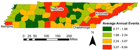
3.2. Patterns of Extreme Weather Event Frequency

Observation of county-level historic extreme weather event frequencies, as described earlier, provided insight into how often a specific event has occurred in a particular area. It was recognized that cold weather (italicized words refer to definitons listed in Table 2) has been a rare event, not recorded in many counties. By contrast, with the exception of east Tennessee, the remaining portions of the state have experienced drought conditions on several occasions, with the most prevalent areas located in the western part of the state and across a north-south swath in middle Tennessee. These droughts are rated D2 (severe drought) or higher, and represent incidences of extreme weather according to the NWS definitions. Historically, damaging hail and lightning, although frequently observed, follow a somewhat random geographical pattern in terms of the frequency of such events. Hot temperature events reflect a pattern that would be considered intuitive for Tennessee given its varied topography, with a higher reported frequency for the middle and western portions of the state than in the more mountainous east. Twister events have been experienced in every county in the state, with more of these occurrences having been reported for middle and west Tennessee, where temperatures are generally warmer and the topography more conducive to tornado destruction. Winter extreme weather events have been most prevalent in the Smoky Mountain region of east Tennessee and along portions of the Cumberland Plateau in the eastern part of middle Tennessee.

The most frequently occurring extreme weather types in Tennessee have been hydrologic, wind, and winter events, with an example of event frequencies for hydrologic events in Figure 4. Heavy precipitation and various forms of flooding have been experienced more than a dozen times in nearly every Tennessee county. Areas where such events have been most commonly observed (i.e., multiple times annually) are a region comprised of counties located in middle Tennessee and select other counties within the state, particularly Shelby County in the south-western part of the state. Various forms of damaging straight-line winds have posed a significant hazard to all counties within the state. The east and middle Tennessee regions, along with Shelby County, are most heavily represented in this regard. Although all counties in the state experience a winter event on average at least once a year, the dominant area of occurrence, as expected, is in the mountainous topograpy of east Tennessee.

By aggregating across all extreme weather categories, one can generate the average number of annual extreme weather events by county, as shown in Figure 5. Typically, storm events entered in the NWS Storm database are categorized by a single event name/type that “most accurately describes the meterological event” (National Weather Service, 2007 [39]). However, although unusual, it is possible for a single meterological event to be recorded more than once in the database under different event type names (e.g., Tornado AND Heavy Rain). This implies that some double-counting of event occurrences is possible during aggregation. While recognizing the potential for introduction of double-counting errors produced by aggregation, this problem was deemed to be minor in comparison to the value that aggregation provides in recognizing counties with moderate frequencies of multiple event types.

The results of aggregating the average annual events across all extreme weather categories as shown in Figure 5 support the obvious conclusion that every county in Tennessee experiences several extreme weather events in a typical year, a clear indication that no location in the state is immune from the hazards associated with extreme weather. However, two counties, Davidson and Shelby counties, stand out in terms of the expected number of such events. The high reported frequency of extreme weather events in these locationss are likely a reflection of the high populations and concentrations of infrastructure in these counties, which are home to the large metropolitan areas of Nashville and Memphis.

Depending on the goals of the particular screening assessment, attempts to normalize NWS event reports by population should be carefully considered before implementation, as the use of thresholds in NWS reporting implies that the relationship between population and event reporting is non-linear. In addition, in rural areas with high levels of agricultural production, a relatively high number of events, with respect to population, may also be recorded in the NWS database due to crop damages incurred. These characteristics of NWS extreme weather event data suggest that use of a simple normalization by population scheme will not correct reporting biases, but will skew results towards rural areas with high levels of agricultural production, hence no better reflecting the underlying weather event patterns than the raw NWS event data. Accordingly, we did not normalize for population in this study.

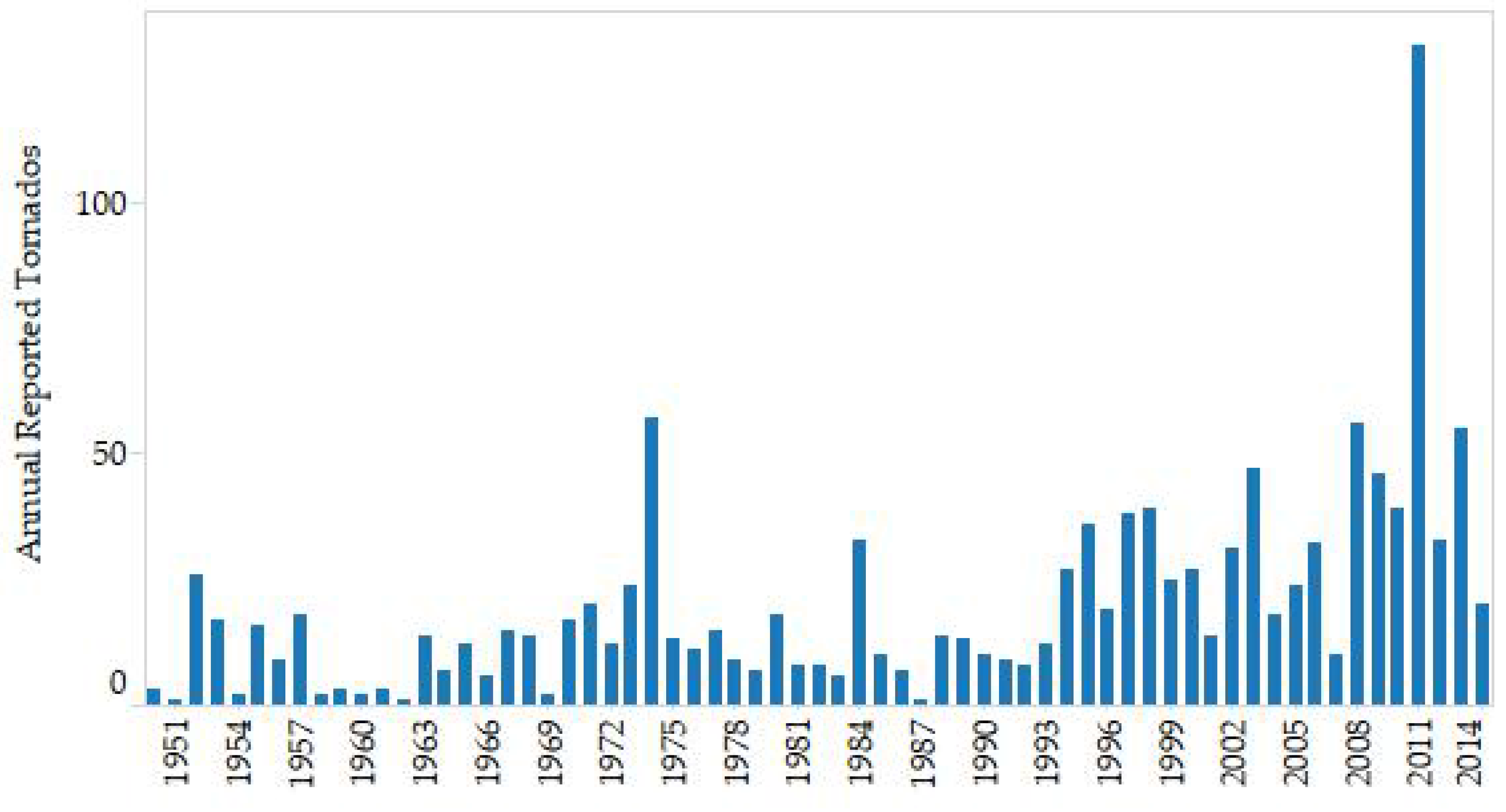
3.3. Example of Trend Analysis: Statewide Wind Event

The analysis of trends in reported extreme weather events in Tennessee provides an understanding of how the number of damaging events has changed over time and may provide insight into future trends not readily available in the CMIP climate models. The purpose of this trend analysis is to identify any potential increases or decreases in annual event frequency rate. For the Tennessee case study, trend analysis was conducted only for tornado and thunderstorm wind events due to lack of sufficient data (more than 40 years) for other extreme weather events in the NWS database. For thunderstorm winds and tornados, the annual number of reported events was plotted by year for the period ranging from 1950 through 2014. Figure 6 shows the annual number of reported tornados in Tennessee. In both cases (thunderstorm winds [not shown in Figure 6] and tornados), plots of the raw data revealed that there has been a pronounced increase in annual event frequency, particularly over the past couple of decades.

Some of these increases in reported thunderstorm wind and tornado events may be attributed to non-climate and weather related variables, such as more rigorous monitoring/recording practices (e.g., advances in recording technologies) and expansion of populous areas (increasing the number of events that trigger the NWS damage reporting threshold). While the impact of these confounding factors on climate and weather trend analyses cannot be entirely accounted for, the most significant effects attributable to changes in monitoring technologies were taken into consideration in the time series analysis. Due to non-stationarity in the datasets (the mean and the variance of the series is not stable over time), transformation of the data was necessary to reconcile data occurring before and after significant change points. Before conducting a trend analysis, non-stationarity change-points in the data were identified using a beta version of the now available US Army Corps of Engineers Nonstationarity Detection Tool with default sensitivity parameter values (U.S. Army Corps of Engineers, 2016 [49]). Three change point statistics (Bayesian Change Point (BCP), Change Point Model (CPM), and Energy Based Divisive Method (ECP)) were used to identify points in the time series where a significant shift in the mean, variance, or distribution of the data occurred (U.S. Army Corps of Engineers, 2016 [49]). One significant change point, which is most likely related to the expansion of Doppler radar-based storm detection, was identified in the data between the years 1993 and 1995 using all three methods (US Department of Commerce, 2016 [50]). The time series were then separated into two subsets at the change point (1994) and data were transformed by multiplying original values by the ratio of the means of the two subsets. The normalized time series was then checked for significant autocorrelation and partial autocorrelation to ensure that a linear least squares regression model was appropriate. The time series exhibited a weak autocorrelation structure; however, examination of the partial autocorrelation structure indicated that an autoregressive model was not appropriate, as lags greater than zero were non-significant (Natrella, 2010 [51]). Therefore, a linear regression (normalized annual reported tornados as the dependent variable and year as the independent variable) was conducted to examine the temporal trends in reported wind events, shown in Figure 7. For the purposes of screening assessments, the slope of the trend line calculated using this relatively simple method can then be used as a multiplier in calculating future vulnerability scores (Guan, 2009 [52]). Where the trend line is statistically insignificant, or the planning horizon is of a significantly long time frame, extrapolation of trends from historical data may not be representative of future trends. In these cases, historical data should be used to arrive at only current, rather than future, vulnerability scores.

While this analysis was conducted at the state rather than county level (due to lack of consistent records at county level across time), and therefore does not provide county level differentiation, in the context of a screening level vulnerability assessment, a state wide trend analysis can still provide differentiation between extreme weather event types by offering insight into whether wind events are trending towards being more or less of a problem in the future. For example, in Tennessee wind events associated with storms, including tornados, are some of the most destructive forces for the transportation system (Camp et al., 2016 [48]). As the trend analysis indicates that the positive trend in tornado events for Tennessee is not significant, planners may decide to prioritize analysis of different extreme weather events that are anticipated to change significantly in the future (e.g., extreme high temperatures).

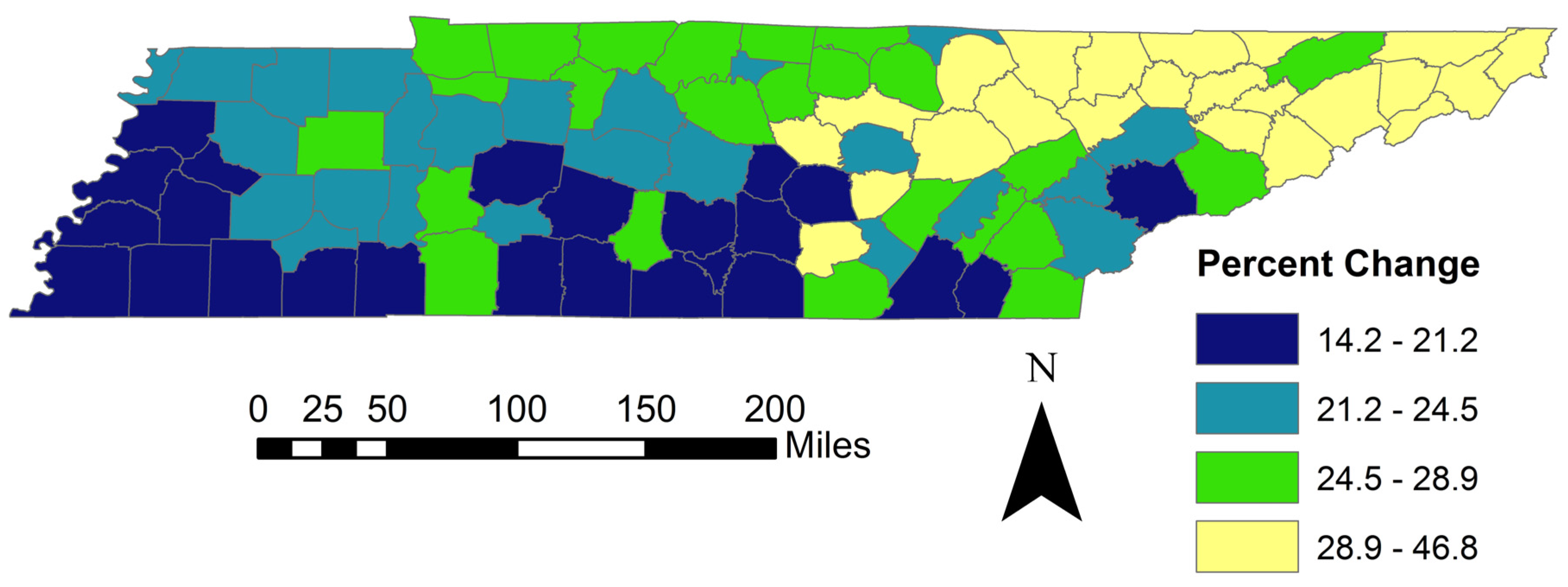
3.4. Future Climate Projections

The available climate models described earlier provide projections for precipitation and temperature. Examination of the net change in these climate variables that each county could be expected to experience in the future provides insight into how extreme weather event frequencies and/or severity are likely to change over time. For example, the frequency and/or severity of hydrologic events such as flooding might be expected to increase between the present and the planning period horizon in counties in which precipitation extremes are predicted to increase. The southern portions of Tennessee and much of the Cumberland Plateau are expected to see low precipitation periods that are even drier than today, suggesting a growing concern of future drought in these areas. Interestingly, many of these same locations are also expected to experience high precipitation periods that are wetter than today (see Figure 3). This suggests that these areas may see more short duration, intense heavy precipitation events with longer periods of dryness in between, which is consistent with observed trends across the nation (U.S. Global Change Research Program, 2014 [53]).

This combination of long dry periods interspersed with intense heavy precipitation can be particularly troublesome in terms of the ability of the ground to absorb water. During periods of drought, soils tend to dry out and harden, reducing the infiltration rate of water from the surface to the soil subsurface, and leading to increased runoff volume during precipitation events (Morin, 1977 [54]). Therefore, when heavy precipitation events follow drought conditions, flooding and flash flooding can more readily ensue, exacerbating conditions that encourage rockslides. This drought-induced reduction in the ability of the soil to quickly absorb excess water is of particular concern where soil is compacted, as compaction also reduces the capacity of the soil to absorb water. This is a concern for any infrastructure, including transportation, because compacting the soil to stabilize foundations is a common practice.

Regarding future temperature conditions, Figure 2 provides a profile of dramatic warming expected to occur across the entire state, such that the coldest periods may be much warmer than they are now. The most significant warming is expected to occur in northeastern Tennessee, which has experienced the most frequent winter weather events. This may result in less concern for winter weather vulnerability in that region. In addition, some warming will also occur throughout the state for the hottest periods of the year.

Recognizing that most critical transportation assets are located in or near highly-urbanized areas in Tennessee, the FHWA Climate Data Processing Tool was utilized to provide a more detailed assessment of future precipitation and temperature extremes in the state’s four major cities: Chattanooga (Hamilton County), Knoxville (Knox County), Memphis (Shelby County), and Nashville (Davidson County) (see Figure 1 for locations). CMIP5 data from the FHWA tool was used to run projections for these cities. All 20 available climate models in the FHWA tool were considered in obtaining the most robust current data available, and to reduce biases that may be present in any one model. Consistent with the more general county-level data, downscaled projections for these urban areas showed significant increases in temperature and precipitation. One example of an excerpt from the CMIP5 output data generated from the FHWA tool is shown in Figure 8, which displays temperature projections for the Memphis area through the middle of the century. The tool also displays end of century results, and additional data points not shown in Figure 9 such as extreme cold, including lowest 4-day average winter temperatures and information regarding the freeze-thaw cycle, which can be especially important with respect to pavement conditions.

One of the advantages of the FHWA tool output is the easily made comparisons between current observed data, mid-century, and end of century projections. These comparisons can provide important insight into not only what planners should expect in the future, but how far those conditions may vary from the current environment planners are more experienced with addressing. This type of detailed analysis facilitated by the FHWA tool can also be used to obtain a robust analysis of climate projections on a more refined scale in areas that may appear vulnerable after undertaking the screening level assessment approach.

Given the local nature of the climate projections from the FHWA tool, these results may be used by regional and local planners to further understand projected precipitation and temperature extremes on a scale not available in a statewide approach. Again, however, design or development of adaptation measures for transportation infrastructure should not rely solely on such downscaled data because of the uncertainty in its reliability at such a fine resolution. Localized high resolution climate projections obtained using the FHWA tool may contain localized errors and should be compared for consistency with coarser resolution averages of downscaled climate projections, such as the county-level dataset used in this study.

Although the climate models are consistently projecting average increases in temperature, much of the middle and eastern portion of the United States has recently experienced some of the coldest temperatures on record. Tennessee also has experienced some record breaking cold temperatures and winter weather events, leading to substantial road damage from potholes in the winter of 2015 and major water line breaks in January 2010. It has been conjectured that anthropogenic-induced warming in the Arctic and loss of sea ice may cause a shift in the jet-stream that brings colder temperatures and more extreme weather generally to the middle latitudes including the eastern and southeastern U.S. (Tang, 2013 [55] and Screen, 2015 [56]). However, this area of research is in its infancy and there is currently no scientific consensus regarding the validity of this hypothesis (Barnes, 2015 [57]). Developments in this field should continue to be watched and project results modified if consensus develops in the scientific community around these considerations.

3.5. Utilizing the Results

The approach described in this paper provides planners and infrastructure managers with a method by which to better understand what types of extreme weather events an area may experience in the future, trends associated with these events, and what climatic changes are projected with respect to precipitation and temperature. Overlaying the location of critical assets on maps displaying areas that currently experience more frequent extreme weather events and that are likely to see a significant shift in climate variables such as precipitation or temperature in the future can convey to planners the areas that may warrant a more detailed analysis. However, assessing the impact these weather events and climate changes may have on particular assets in order to better quantify vulnerability and risk is a more comprehensive task.

Assessing impacts can be one of the most difficult aspects to understanding vulnerabilities and ultimately to choosing effective and economical adaptation measures. With respect to natural disasters, it can often be difficult determine which type is the most harmful—and if so how harmful—to a particular asset or network (Sohn, 2006 [58]). If the study area is large geographically, such as an entire state, assessing impacts can be even more difficult where characteristics of individual assets (such as pavement binder used in the case of roads, historical response to hazards, or bridge elevation) cannot realistically be taken into account initially. To assess impacts at this scale, the project designed and administered a comprehensive online survey in which a broad range of transportation experts, geographically spread across the state, were enlisted to complete (Camp et al., 2016 [48]). For each asset type selected, the survey presented a series of extreme weather scenarios adapted from the National Weather Service definitions. For example, one weather event scenario included “sustained winds ≥40 mph for ≥1 h or ≥58 mph for any duration.”

The transportation experts were then asked to evaluate the impacts (the level of asset damage or system disruption caused by the selected weather event) according to a four-point qualitative scale (nominal, moderate, significant, or catastrophic). The qualitative damage/disruption rankings were then converted into a numerical score by assigning values as follows: nominal = 1, moderate = 2, significant = 3 and catastrophic = 4. The response values were aggregated into the extreme weather event categories as defined in Table 2 such that all the survey response values for multiple weather scenarios within one weather category (e.g., both sustained winds over 40 mph and sustained winds 25–39 mph with larger gusts would be aggregated to produce a single impact score for wind), and an average impact score was then generated for each asset type and weather event combination based on the number of responses that were completed (Camp et al., 2016 [48]).

Developing a method to combine the results of the impact survey with the county-level climate and weather data resulted in overall vulnerability scores that provide a valuable vulnerability screening assessment tool to determine what assets or areas to review more closely for potential vulnerability or adaptation initiatives.

Vulnerability scores were calculated on a county basis. Multiplying the impact score (for each asset/event combination) by a county’s annual event frequency for that event results in a current vulnerability score. Multiplying the current vulnerability score by the slope of the line generated by the trend analysis (for extreme weather events) or by the percent increase/decrease (for projected climate variables), depending on the relevancy of the factor to the weather event type, provides future vulnerability scores. For example, if future vulnerability scores are being calculated for hydrologic events, the current vulnerability scores should be multiplied by the percent increase in the 90th percentile (high) precipitation values.

In applying this method, a vulnerability score by asset/weather event combination for each county was derived. An additional vulnerability score was generated as the sum of vulnerability scores taken across all weather/climate events. This added step provides an opportunity to identify those counties that may not have high vulnerability for any one asset/event combination, but may be vulnerable across a wide range of weather event/asset combinations, potentially warranting a more detailed examination. A more detailed summary of the methodology utilized to calculate vulnerability scores appears in

Table 3. Summary of methodology for calculating county level vulnerability scores derived from impact scores, weather event frequencies, and climate/weather data trends.

1	Obtain “impact value” for each infrastructure/weather event combination. For each infrastructure type, average the survey results regarding impact (range from 1–4) for that particular hazard (weather event) and infrastructure type (e.g., locks). This produces a numerical value—the “impact value” for each hazard/asset type combination indicating the impact to each infrastructure type when exposed to the particular weather event type (column two from Table 2).
2	Obtain current vulnerability scores (impact value x frequency). For each county, multiply the average annual frequency of each aggregated weather event (column one from Table 2) times the aggregated weather event impact score for that infrastructure/weather event combination.
3	Obtain future vulnerability scores. Take the current vulnerability scores and apply percent increase/decrease for precipitation and temperature, and/or regression slope for future straight-line wind and tornado frequencies where these factors are relevant to the weather event type.
4	Rank counties by future vulnerability scores. Assign each spatial unit (e.g., county) a vulnerability score ranking by asset/weather event combination based on the value of a units vulnerability score relative to other units. Add an additional category ranking the sum of future vulnerability scores across all aggregate extreme weather event types to account for those counties that may not have high vulnerability rankings in any one infrastructure/weather event combination, but where infrastructure is likely to be exposed and damaged from a significant number of different weather events.

.

The process outlined in Table 3 results in vulnerability scores with a county-based spatial resolution for each unique weather/asset combination. Once the vulnerability information is spatially displayed, overlaying the locations of the assets of concern will identify where these assets may have the greatest potential vulnerability. Unlike a more detailed approach to obtaining vulnerability scores that is often described in the literature (Smit & Wandel, 2006 [18]), this approach is a screening tool, enabling planners to identify where it might be appropriate to undertake a more comprehensive analysis. Those more refined vulnerability assessments are often better suited to understanding the vulnerabilities of a few select assets because they can include very specific information about the asset that may make it more or less vulnerable to a chosen impact (such as pavement binder, age, current condition, elevation, etc.), and include sophisticated analyses in which different aspects related to vulnerability may be weighted to produce vulnerability scores and rankings within a group of selected assets (such as road segments or bridges). The FHWA Vulnerability Assessment Scoring Tool (VAST) is one such tool that could be used to more precisely score and rank vulnerability information about assets that show potential vulnerability through the screening approach discussed herein (FHWA, 2015) [59]). The promise of the method described in this paper is that planners responsible for a large number of assets can readily locate the assets that may warrant a more detailed study.

As an example, Figure 9 displays a map showing the vulnerability scores by county for locks exposed to an extreme hydrologic event—the counties in red are those with the highest vulnerability scores. Adding the actual location of the critical lock assets to this map quickly conveys important information regarding vulnerabilities—only the counties in red (which indicate an area of potential exposure and high impact) that actually have locks within their boundaries may warrant a further assessment of vulnerabilities. Depending on resources and goals, the locks appearing in counties in orange may also be targeted for further analysis. The same approach can be taken for each asset and weather event combination, communicating visually which assets may warrant a more detailed review.

4. Conclusions

The methods for applying climate and weather data to vulnerability screening assessments developed in this study are easily transferable to other organizations that are interested in understanding the potential impact of extreme weather and climate change on assets over the course of the next two decades. The NWS historic weather data is available for locations across the country and can be used to better understand historic weather patterns, often going back 65 years. Although the downscaled CMIP3 climate projections compiled by the University of Georgia researchers are only available for counties in the southeastern United States, some agencies may not want county level data and there are other available approaches to obtaining downscaled climate data. For example, the FHWA CMIP Climate Data Processing Tool was developed with transportation planners in mind but provides meaningful and easily understandable data likely to be useful well beyond the transportation context and also may be valuable for work done on a smaller scale than a statewide study. The tool includes the raw daily CMIP data (both observed and projections) for the location analyzed which can be manipulated to support the goals of the particular study (e.g., if the identification of certain trends, such as percentage increase or decrease, are desired). Additionally, because counties in some areas, especially in the Western United States, may be too large to obtain data that can be compared at the county level, the North American Regional Climate Change Assessment Program (NARCCAP) provides downscaled data at 50 kilometer resolution, a size conducive for use with the screening approach presented in this paper (NARCCAP, 2016 [60]). Finally, the National Center for Atmospheric Research (NCAR) and others are currently developing tools to better assist decision makers in understanding the climate risks they may face (NCAR, 2016 [61]). For example, the Global Risk, Resilience, and Impacts Toolbox (GRITT) is currently under development at NCAR to assist extreme weather and climate change risk management and adaptation decision making, and is intended to be useful across a variety of sectors. Also, Schweikert has detailed the benefits of the Infrastructure Planning Support System (IPSS) that can be used to help quantify the climate change impacts to specific roads using input by local planners and improve adaptation decisions (Schweikert, 2014 [62]).

These tools and approaches are particularly important as vulnerability assessments are in their infancy and many planners have found it difficult to obtain and use climate data in a meaningful way when attempting to understand impacts. As planners are faced with the need to address more severe, and ever increasing, climate and weather-related risks to public and private assets, techniques such as the one described herein can help facilitate the optimal allocation of limited resources to mitigate risks.

References

1. T. Pollard. “Damage Control: Adapting Transportation to a Changing Climate.” William Mary Environ. Law Policy Rev. 365 (2015): 370–377. [Google Scholar]
2. C. Schulz. “Identification of Critical Transport Infrastructures, Climate Change and Vulnerability: Challenges for Spatial Planning and Civil Protection.” Available online: http://www.cedim.de/download/14_Schulz.pdf (accessed 28 July 2016).
3. M. Savonis, S.V. Burkett, and J. Potter. “Impacts of Climate Change and Variability on Transportation Systems and Infrastructure: Gulf Coast Study, Phase I. ” Available online: http://climate.dot.gov/documents/gulf_coast_study.pdf (accessed on 28 July 2016).
4. TRB. Transportation Research Board Special Report 290, Potential Impacts of Climate Change on U.S. Transportation. Washington, DC, USA: TRB, 2008. [Google Scholar]
5. TRB NCHRP. Transportation Research Board, National Cooperative Highway Research Program, Report 750, Volume 2—Climate Change, Extreme Weather Events, and the Highway System: Practitioner’s Guide and Research Report. Washington, DC, USA: TRB, 2014. [Google Scholar]
6. FHWA. “Federal Highways Administration, Climate Change Resilience Pilots. ” Available online: http://www.fhwa.dot.gov/environment/climate_change/adaptation/resilience_pilots/index.cfm (accessed on 6 June 2016).
7. FHWA. “Federal Highway Administration, Climate Change and Extreme Weather Vulnerability Assessment Framework, No. FHWA-HEP-13-005. ” Available online: http://www.fhwa.dot.gov/environment/climate_change/adaptation/publications/vulnerability_assessment_framework/fhwahep13005.pdf (accessed on 28 July 2016).
8. V.L. Knoop, M. Snelder, H.J. Van Zuylen, and S.P. Hoogendoorn. “Link-level Vulnerability Indicators for Real-World Network.” Transp. Res. Part A 46 (2012): 843–854. [Google Scholar] [CrossRef]
9. M. Taylor, and G. D’Este. Transport Network Vulnerability: A Method for Diagnosis of Critical Locations in Transport Infrastructure Systems. Heidelberg, Germany: Springer, 2007. [Google Scholar]
10. A. Erath, J. Birdsall, K.W. Axhausen, and R. Hajdin. “Vulnerability assessment methodology for Swiss road network.” Transp. Res. Rec. 2137 (2010): 118–126. [Google Scholar] [CrossRef]
11. J.E. Jenelius. “Incorporating dynamics and information in a consequence model for road network vulnerability analysis.” In Proceedings of the Third International Symposium on Transport Network Reliability, The Hague, The Netherlands, 19–20 July 2007.
12. V.L. Knoop, S.P. Hoogendoorn, and H.J. Van Zuylen. “The influence of spillback modeling when assessing consequences of blockings in a road network.” Eur. J. Transp. Infrastruct. Res. 8 (2008): 287–300. [Google Scholar]
13. M.A.P. Taylor, S.V.C. Sehkar, and G.M. D’Este. “Application of accessibility based methods for vulnerability analysis of strategic road networks.” Netw. Spatial Econ. 6 (2006): 267–291. [Google Scholar] [CrossRef]
14. O. Berle, B. Asbjornslett, and J. Rice. “Formal Vulnerability Assessment of a maritime transportation system.” Reliab. Eng. Syst. Saf. 96 (2011): 696–705. [Google Scholar] [CrossRef] [Green Version]
15. E. Jenelius, T. Petersen, and L.-G. Mattsson. “Importance and exposure in road network vulnerability analysis.” Transp. Res. Part A Policy Pract. 40 (2006): 537–560. [Google Scholar] [CrossRef]
16. FHWA. “Federal Highway Administration, Impacts of Climate Change and Variability on Transportation Systems and Infrastructure: The Gulf Coast Study, No. FHWA-HEP-11–019. ” Available online: http://www.fhwa.dot.gov/environment/climate_change/adaptation/ongoing_and_current_research/gulf_coast_study/gcs.cfm (accessed on 6 June 2016).
17. FHWA. “Federal Highway Administration, Gulf Coast Study, Phase 2 Case Study, FHWA-HEP-14–053. ” Available online: https://www.fhwa.dot.gov/environment/climate_change/adaptation/case_studies/gulf_coast_study/ (accessed on 23 May 2016).
18. S. Wandel. “Adaptation, Adaptive Capacity and Vulnerability.” Glob. Environ. Chang. 16 (2006): 282–292. [Google Scholar]
19. P.M. Kelley, and W.N. Adger. “Theory and practice in assessing vulnerability to climate change and facilitating adaptation.” Clim. Chang. 47 (2000): 325–352. [Google Scholar] [CrossRef]
20. S. Xenarios, S. Xenarios, A. Nemes, G. Sarker, and N. Sekhar. “Assessing vulnerability to climate change: Are communities in flood-prone areas in Bangledesh more vulnerable than those in drought-prone areas? ” Water Resour. Rural Dev. 7 (2016): 1–19. [Google Scholar] [CrossRef]
21. H. Füssel. “Review and Quantitative Analysis of Indices of Climate Change Exposure, Adaptive Capacity, Sensitivity, and Impacts.” World Development Report: Development and Climate Change. 17 August 2009. Available online: http://lacer.lacea.org/handle/10986/9193 (accessed on 3 June 2016).
22. IPCC. Intergovernmental Panel on Climate Change. Climate Change 2007: Climate Change Impacts, Adaptation, and Vulnerability. Cambridge, UK: Cambridge University Press, 2007. [Google Scholar]
23. United States Agency for International Development (USAID). Spatial Climate Change Vulnerability Assessments: A Review of Data, Methods, and Issues; Washington, DC, USA: USAID, 2014.
24. M. Abkowitz. “Identifying Critical Transportation Assets in Performing Extreme Weather Vulnerability Assessments: The Tennessee Experience.” Case Stud. Transp. Policy, 2016, under review. [Google Scholar]
25. T.J. Kim, and J.S. Lee. “Development of Index for Identifying Critical Transportation Links.” In Symposium: Entrepreneurship and Development-Local Processes and Global Patterns. Edited by I. Johansson. Trollhättan, Sweden: University West, 2006. [Google Scholar]
26. E. Mistakis, A. Papanikolaou, G. Ayfadopoulou, J. Salanova, C. Doll, G. Giannopolous, and C. Zerefos. “An integrated framework for linking climate change impacts to emergency adaptation strategies for transport networks.” Eur. Transport Res. Rev. 6 (2014): 103–111. [Google Scholar]
27. ACSE. “American Society of Civil Engineers, Committee on Adapting to a Changing Climate: Adapting Infrastructure and Civil Engineering Practice to a Changing Climate, 2015.” Available online: http://ascelibrary.org/doi/pdf/10.1061/9780784479193 (accessed on 12 June 2016).
28. M. Meyer. “Design Standards for U.S. Transportation Infrastructure: The Implications of Climate Change, Georgia Institute of Technology, 18 December 2006; Commissioned Paper for Transportation Research Board Special Report 290, Potential Impacts of Climate Change on U.S. Transportation, 2008.” Available online: http://onlinepubs.trb.org/onlinepubs/sr/sr290Meyer.pdf (accessed on 28 July 2016).
29. D. Archer. Global Warming: Understanding the Forecast, 2nd ed. Hoboken, NJ, USA: John Wiley & Sons, 2011, p. 57. [Google Scholar]
30. FHWA. “Federal Highway Administration; Literature Review: Climate Change Vulnerability Assessment, Risk Assessment, and Adaptation Approaches, Prepared for FHWA by ICF International, 24 July 2009. ” Available online: https://www.fhwa.dot.gov/environment/climate_change/adaptation/publications/vulnerability_assessment/ (accessed on 28 July 2016).
31. S. Chernicoff, and D. Whitney. Geology, 4th ed. Upper Saddle River, NJ, USA: Prentice Hall, 2007. [Google Scholar]
32. National Oceanic and Atmospheric Administration (NOAA). “Sea Level Rise Modeling, 2015. ” Available online: http://www.nauticalcharts.noaa.gov/csdl/sealevelrise.html (accessed on 12 June 2015).
33. T. Wall, M. Rodgers, and A. Amekudzi. “Projecting Climate Change impacts on the Transportation System: A GIS based approach for network-level culvert infrastructure management.” In Proceedings of the Transportation Research Board 2014 Annual Meeting, Washington, DC, USA, 15 January 2014.
34. “Downscaling Climate Data, University of British Columbia, 2008.” Available online: http://www.climate-decisions.org/2_Downscaling%20Climate%20Data.htm (accessed on 18 November 2015).
35. Intergovernmental Panel on Climate Change (IPCC). “Climate Change 2013: The physical science basis.” In Working Group I Contribution to the Fifth Assessment Report of the IPCC. Geneva, Switzerland: IPCC, 2013. [Google Scholar]
36. L. Condon, L. Condon, S. Gangopadhyay, and T. Pruitt. “Climate Change and non-stationary flood risk for the upper Truckee River Basin, 12 January 2015.” Hydrol. Earth Syst. Sci. 19 (2015): 159–175. [Google Scholar] [CrossRef]
37. Federal Highway Administration (FHWA). The Use of Climate Information in Vulnerability Assessments, FHWA-HEP-12–010; Washington, DC, USA: FHWA, 2011.
38. “Washington State Department of Transportation, Climate Impacts Vulnerability Assessment. ” Available online: http://www.wsdot.wa.gov/NR/rdonlyres/B290651B-24FD-40EC-BEC3-EE5097ED0618/0/WSDOTClimateImpactsVulnerabilityAssessmentforFHWAFinal.pdf (accessed on 12 June 2016).
39. National Weather Service (NWS). Storm Data Preparation, Instruction 10–1605, NWSPD 10–16. Silver Spring, MD, USA: National Weather Service, 2007. [Google Scholar]
40. NOAA. “National Oceanic and Atmospheric Administration, Storm Events Database. ” Available online: http://www.ncdc.noaa.gov/stormevents/ (accessed on 31 May 2015).
41. M. Downton, J. Miller, and R. Pielke. “Reanalysis of U.S. National Weather Service Flood Loss Database.” Nat. Hazards Rev. 6 (2005): 13–22. [Google Scholar] [CrossRef]
42. M. Gall, K.A. Borden, and S.L. Cutter. “When Do Losses Count? Six Fallacies of Natural Hazards Loss Data.” Am. Meteorol. Soc. 90 (2009): 799–809. [Google Scholar] [CrossRef]
43. S. Kulkarni, and H. Huang. “Changes in Surface Wind Speed over North America from CMIP5 Model Projections and Implications for Wind Energy.” Adv. Meteorol. 2014 (2014): 292768. [Google Scholar] [CrossRef]
44. WCRP. “World Climate Research Programme, Working Group on Coupled Modeling, Coupled Model Intercomparison Project (CMIP3 and CMIP5), Information.” Available online: http://www.wcrp-climate.org/wgcm/ (accessed on 12 June 2016).
45. Federal Highway Administration (FHWA). U.S. DOT CMIP Climate Data Processing Tool, User’s Guide; Washington, DC, USA: FHWA, 2014.
46. E. Maurer, L. Brekke, T. Pruitt, and P. Duffy. “Fine-Resolution Climate Projections Enhance Regional Climate Change Impact Studies.” Eos Trans. AGU 88 (2007): 504, Data Creator: Thomas L. Mote, Department of Geography, University of Georgia, Athens, GA, USA, 2007. [Google Scholar] [CrossRef]
47. ICF International. “CMIP Climate Data Processing Tool and Sensitivity Matrix, developed as part of the Gulf Coast Study, Phase 2 for the U.S. Department of Transportation, Center for Climate Change and Environmental Forecasting. ” Available online: http://www.fhwa.dot.gov/environment/climate_change/adaptation/publications_and_tools/ (accessed on 12 June 2016).
48. J. Camp. “Assessing the Impacts of Extreme Weather on Critical Transportation Assets: An Expert Elicitation Approach; forthcoming paper on expert elicitation in climate change and extreme weather impact analysis.” Transp. Res. Part D Transp. Environ. 2016, under review. [Google Scholar]
49. U.S. Army Corps of Engineers. “Nonstationarity Detection Tool, User Guide.” Available online: http://corpsmapu.usace.army.mil/rcc/nsd/docs/Nonstationarity_Detection_Tool_User_Guide.pdf (accessed on 26 April 2016).
50. US Department of Commerce. “History of the National Weather Service in Nashville, Tennessee. ” Available online: http://www.srh.noaa.gov/ohx/?n=nwshistory (accessed on 15 June 2016).
51. M. Natrella. “NIST/SEMATECH e-handbook of statistical methods, 2010. ” Available online: http://www.itl.nist.gov/div898/handbook/index.htm (accessed on 12 June 2016).
52. L. Guan. “Preparation of future weather data to study the impact of climate change on buildings.” Build. Environ. 44 (2009): 793–800. [Google Scholar] [CrossRef]
53. “United States Global Change Research Program.” In Proceedings of the Third National Climate Assessment, Washington, DC, USA, 6 May 2014.
54. J. Morin, and Y. Benyamini. “Rainfall Infiltration into Bare Soils.” Water Resour. Res. 13 (1977): 813–817. [Google Scholar] [CrossRef]
55. Q. Tang, X. Zhang, X. Yang, and J. Francis. “Cold Weather Extremes in Northern Continents Linked to Arctic Sea Ice Loss.” Environ. Res. Lett. 8 (2013): 014036. [Google Scholar] [CrossRef]
56. J. Screen, C. Deser, and L. Sun. Projected Changes in Regional Climate Extremes Arising from Arctic Sea Ice Loss. Manuscript submitted to Environmental Research Letters. 7 May 2015. Available online: http://www.cgd.ucar.edu/staff/cdeser/docs/submitted.screen.reg_climate_extremes.may15.pdf (accessed on 12 June 2016).
57. E. Barnes, and J. Screen. “The Impact of Arctic Warming on the Midlatitude Jet-Stream: Can it? Has it? Will it? ” Wiley Interdiscip. Rev.: Clim. Chang. 6 (2015): 277–286. [Google Scholar] [CrossRef] [Green Version]
58. J. Sohn. “Evaluating the significance of highway network links under the flood damage: An accessibility approach.” Transp. Res. Part A Policy Pract. 40 (2006): 491–506. [Google Scholar] [CrossRef]
59. FHWA. “Federal Highway Administration, U.S. DOT Vulnerability Assessment Scoring Tool, User’s Guide, 2015. ” Available online: https://www.fhwa.dot.gov/environment/climate_change/adaptation/adaptation_framework/modules/scoring_tools_guide/vast_users_guide.pdf (accessed on 24 May 2016).
60. NARCCAP. “North American Regional Climate Change Assessment Program, 2016.” Available online: http://www.narccap.ucar.edu/ (accessed on 22 June 2016).
61. NCAR. “National Center for Atmospheric Research, 2016.” Available online: https://ncar.ucar.edu/about-ncar (accessed on 22 June 2016).
62. A. Schweikert, P. Chinowsky, K. Kwiatkowski, and E. Xavier. “The Infrastructure Planning Support System: Analyzing the impact of climate change on road infrastructure and development.” Transp. Policy 35 (2014): 146–153. [Google Scholar] [CrossRef]
Figure 1. Average annual wind events by county. Frequencies are mapped by quartiles where red indicates realtively high event frequency and dark green relatively low event frequency.
Risks 04 00028 g001
Figure 2. Percentage change between observed (2000–2010) and projected (2035–2045) 10th percentile (low) temperature values. Percentage change is mapped in quartiles, where yellow indicates a relatively large increase and dark blue indicates a relatively small increase, in the temperature during colder months.
Risks 04 00028 g002
Figure 3. Percentage change between observed (2000–2010) and projected (2035–2045) 90th percentile (high) precipitation values. Percentage change is mapped in quartiles, where dark purple indicates a relatively high increase and light purple indicates a slight decrease or small increase, in precipitation during wetter months.
Risks 04 00028 g003
Figure 4. Average annual hydrologic events. Frequencies are mapped by quartiles where red indicates a relatively high frequency and dark green indicates a relatively low frequency.
Risks 04 00028 g004
Figure 5. Average annual extreme weather events (mapped by quantiles).
Risks 04 00028 g005
Figure 6. Annual reported tornado events in Tennessee between 1950 and 2014.
Risks 04 00028 g006
Figure 7. Trend analysis of normalized annual reported tornados in Tennessee. The trend line (non-significant for this example) is displayed as a thick gray line and thin, curved, gray lines represent 95% confidence bands.
Risks 04 00028 g007
Figure 8. Excerpt of CMIP5 downscaled projected climate data analysis using the FWHA Climate Data Processing Tool for Memphis, Tennessee, through mid-century.
Risks 04 00028 g008
Figure 9. Future vulnerability of lock assets to hydrologic events (mapped by quartiles).
Risks 04 00028 g009