
Choosing Markovian Credit Migration Matrices by Nonlinear Optimization


1
Fakultät für Informatik und Mathematik, Hochschule München, Lothstrasse 64, 80335 München, Germany
2
Institut für Mathematik, Universität Augsburg, Universitätsstrasse 2, 86159 Augsburg, Germany
*
Author to whom correspondence should be addressed.
Risks 2016, 4(3), 31; https://doi.org/10.3390/risks4030031
Submission received: 4 July 2016
/
Revised: 12 August 2016
/
Accepted: 22 August 2016
/
Published: 30 August 2016
(This article belongs to the Special Issue Applying Stochastic Models in Practice: Empirics and Numerics)
Abstract
:Transition matrices, containing credit risk information in the form of ratings based on discrete observations, are published annually by rating agencies. A substantial issue arises, as for higher rating classes practically no defaults are observed yielding default probabilities of zero. This does not always reflect reality. To circumvent this shortcoming, estimation techniques in continuous-time can be applied. However, raw default data may not be available at all or not in the desired granularity, leaving the practitioner to rely on given one-year transition matrices. Then, it becomes necessary to transform the one-year transition matrix to a generator matrix. This is known as the embedding problem and can be formulated as a nonlinear optimization problem, minimizing the distance between the exponential of a potential generator matrix and the annual transition matrix. So far, in credit risk-related literature, solving this problem directly has been avoided, but approximations have been preferred instead. In this paper, we show that this problem can be solved numerically with sufficient accuracy, thus rendering approximations unnecessary. Our direct approach via nonlinear optimization allows one to consider further credit risk-relevant constraints. We demonstrate that it is thus possible to choose a proper generator matrix with additional structural properties.
1. Introduction
Numerous methods exist for embedding a given discrete-time (in most cases, one-year) transition matrix into continuous-time, i.e., for finding the (infinitesimal) generator matrix. Simply computing the matrix logarithm does not necessarily result in a valid solution for the generator matrix. This seems especially to be the case for transition matrices in credit risk, where often, the matrix logarithm yields candidates for a generator, but with negative off-diagonal entries. Consequently, one needs to find procedures where, on the one hand, valid generators are produced and, on the other hand, the distance (for the moment using any matrix norm) of its exponential to the given transition matrix is minimal.
Our research mainly follows the work of [1], where the proposed method is also based on optimization. They suggest to avoid solving the true problem of interest, the best approximation of the annual transition matrix (BAM), but instead solving an approximation only, called quasi-optimization of the generator (QOG). For the solution of QOG, they propose the DMPG algorithm (somewhat confusingly called the distance minimization problem for the generator matrix). The DPMG algorithm solves QOG by viewing each row of the transition matrix separately1. Based on a surprising close connection between BAM and QOG, proven by [2], we suggest to solve BAM directly by methods of nonlinear programming based on a starting point obtained by the solution of QOG. To deal with the non-convex structure of BAM, we apply an iterative homogenization procedure to obtain more reliable solutions. This procedure yields quite robust solutions, as accuracy is gained step by step. Although our numerical experiments show no superiority compared to a direct solution of BAM for the considered problem instances, it gives the latter more credibility of being the best solution. Further, we provide a comparison to the diagonal (DA) and weighted adjustment (WA) techniques, which are quite popular techniques in current credit risk applications. In general, the optimization technique allows a more flexible interpretation and various additional applications, as opposed to non-optimization methods (e.g., DA or WA). For instance, constraints enforced by regulators, for example one-year default probabilities, need to be greater or equal to a given threshold or bank internal requirements may be incorporated. More precisely, one further main novelty of our approach lies with the adjustment of default and migration probabilities/rates during the optimization procedure to a specific desired outcome. These extensions are thoroughly investigated in our study.
In this context, it needs to be mentioned that several research papers also exist solely addressing computing the roots of transition matrices, e.g., [3,4,5]. Here, Lin, L. [6] proceeds in her dissertation similarly as in our work by solving the minimization problem as a whole for obtaining an optimal solution of BAM by utilizing MATLAB’s2 inbuilt optimization routines. There, analytic formulas for the gradient and the Hessian matrix of the objective function are derived. Further attention is paid to the choice of the nonlinear optimization method and the choice of the starting point. However, the focus there is on local methods only, with almost no discussion of the global aspects of the problem. More importantly, Lin does not exploit this formulation by adding further highly-relevant credit risk-related constraints.
The remainder of this paper is organized as follows: First, we briefly review existing results on whether the logarithm of a given transition matrix exists and whether the one-year matrix can be embedded into continuous time, which is given in Section 2. These checks are conducted on commonly-used one-year transition matrices in credit risk-relevant assessments, which are published on a regular basis by rating agencies. Section 3 introduces sufficient conditions and additional constraints, as well as the underlying optimization problems. An extensive application in Section 4 compares the underlying techniques and addresses the impact of the additional constraints imposed specifically on present and future default probabilities. Again, transition matrices estimated from real data are utilized for an extensive analysis. In Section 5, a brief summary is given.
2. Transition Matrix Analysis
The common approach, in the context of embedding a transition matrix3 in continuous time, is based on the notion of the generator of a continuous-time Markov process. A generator (or intensity matrix) of a Markov process is a matrix , for which:
and for which the entries are rates at which the Markov process jumps from state i to j, with:
These necessary and sufficient properties of (1) for being a generator matrix can be derived in three different ways, as can be seen in [9]. A formal proof of (1) is given in [10]. In Reference [11], Bielecki, T. and Rutkowski, M. provide this compact definition of the embedding problem:
Definition 1 (Embedding problem).
Find a matrix satisfying (1) (non-negative off-diagonal entries and all rows summing to zero), such that .
As from Definition 1 needs to hold, a feasible candidate may be the matrix logarithm of a given transition matrix. The work in [12] gives two necessary and sufficient conditions on the existence and uniqueness of the matrix logarithm. The existence is given for , and , resulting in a real-valued solution, but not in a valid generator according to (1), as negative off-diagonal values arise. Moreover, in general, the issue of multiple solutions may occur. For example, when computing the eigenvalues of , a complex conjugate eigenvalue pair exists, so that one needs to search in every existing branch of the matrix logarithm for a valid generator. Applying the search algorithm proposed by [13,14], three real-valued solutions of the matrix logarithm exist, yet no valid generator can be found for this particular matrix due to the corresponding smallest off-diagonal entries , and of branches , 0 and 1. At this point, many publications addressing the matter resort to the adjustment techniques (DA and WA) for eliminating negative off-diagonal entries. Both methods are thoroughly described, for example, in [14].
The embedding problem itself relies on more restrictive conditions for obtaining valid generators which consists of the existence of an embeddable matrix in continuous time and its uniqueness (also referred to as identification), reaching back as far as [15]. Thus far, necessary and sufficient conditions have only been formulated for (see [16], attributed to D. G. Kendall, and [17]) and matrices (see [18,19,20,21,22]). For higher dimensions, the issue still remains vague. The work in [6] states a rather complete list of nine necessary conditions in her dissertation, where we only list the most important conditions according to [14]:
Condition 1
(Necessary conditions for the existence of a generator with )
While Conditions (b) and (c) of Condition 1 are satisfied by all given matrices in Table A1, Condition (a) is not. For example, in , it is possible to migrate from Class AAA to CCC-C via Class A ( and ), but not directly, as . This violation is a frequently-observed phenomenon when examining credit risk transition matrices (due to non-observable defaults for high ratings in historical data, as also pointed out in [14]). Therefore, [14] established a more quantitative version of (a), being the most recent condition added to the list, (d). However, the newly-computed lower bounds for the zero entries are not sufficiently large in order to obtain a valid generator, as still negative off-diagonals remain. This finding applies to all three example transition matrices.
It can be concluded that specifically credit risk transition matrices have problems fulfilling conditions on matrix entries, while eigenvalue conditions are usually satisfied. Thus far, we can conclude that typically, no valid generator for transition matrices exist.
3. Optimization Problems
To this end, numerically solving the embedding problem has been investigated in several research papers. A brief chronological listing of regularization-based methods is outlined, before formalizing the optimization problems proposed by [1]. First, regularization techniques of adjusting negative off-diagonal entries, arising when computing the matrix logarithm, can be found in [3,4], where DA and WA are described. A similar procedure is given in the seminal work of [26]. These are further investigated for example in [1,8,14]. The aim of [1] was to solve the optimization problem of the best approximation of the annual transition matrix. BAM is the actual problem to solve; however, it represents a high-dimensional non-convex optimization problem. Thus, [1] replaced the problem by an approximation, now minimizing the sum of squared deviations between and , referred to as quasi-optimization of the generator (QOG). The approximation allowed [1] to solve the problem almost analytically, considering the rows of the input matrix separately (they refer to this algorithm as the distance minimization problem for the generator matrix (DMPG)). Until 2010, it remained open if there were a (weak/strong) relation between BAM and its approximation QOG. Then, [2] derived Condition 2, which gives the distance of any solution of a generator matrix to the matrix logarithm . In the context of optimization, it follows that should be close to , then so is to .
Condition 2.
Let be a transition matrix such that all eigenvalues are strictly positive, and put . If lies within the set of Equation (1) and , then:
where the used norm is .
The first attempt of solving QOG and BAM (the actual problem) as a whole, hence nonlinearly, was conducted by [6] in her dissertation. This has one great advantage over all other methods so far, namely additional credit risk-relevant constraints can be incorporated, which are introduced in the following.
3.1. Constraints
For the optimization problems, we need to define the set of all valid generators; hence, Definition 2 is derived from: (1).
Definition 2 (Generator matrix constraints).
As the main novel idea, we suggest to additionally impose constraints4 specifically addressing credit risk-relevant characteristics. The first constraint (D1) reflects Basel II regulation requirements demanding that one-year default probabilities need to be larger or equal to 3 basis points (bp). Constraint (D2) is a logical continuation and a realistic internal banking requirement stating that default probabilities should be monotonic increasing with decreasing rating classes. Thus, abnormal behaviors as observed in Moody’s transition matrix in Table A1 where can be corrected. While both constraints are optional, (D1) can be seen as necessary from a regulator’s point of view, whereas (D2) can be considered as completely optional.
Definition 3 (Default probability constraints).
Continuing the idea of including additional constraints, we define a constraint specifically for the migration rates from one state to another. Similarly to (D2), we impose a monotonic behavior. For example, it is more probable to migrate from, for example, AAA to AA than from AAA to C, and vice versa. (M1) handles the upper triangular matrix and (M2) the lower triangular matrix, both excluding the main diagonal. Also not included is the default state ‘D’, as it is absorbing; thus, the last column and the last row are omitted from (M1) and (M2), respectively. Taking the rates into consideration has the advantage of being linear constraints, and “jumping too far” is less likely. The migration rate constraints of Definition 4 are again purely optional.
Definition 4 (Migration rate constraints).
Lastly, in our selection of additional constraints, we consider a general monotonic behavior of the rating concept in credit risk. The first state is associated with AAA, being the best rating class and having the least risk. With decreasing ratings, the risk increases. Following [26] (also found in [14]; the corresponding proof is given in [27]), this requirement can be ensured by one of the following two conditions of Condition 3.
Condition 3.
Let be a valid generator for . Then, the following statements are equivalent:
- 1
- is a nondecreasing function of i for every fixed k and
- 2
- for all i, k such that .
An example where the first condition does not apply, we find that with and , the condition is violated for , as and . In [14], Israel, R. B. et al. point out that this violation is frequently observed with given transition matrices. With both conditions being equivalent, the less cumbersome choice for the upcoming optimizations is the second condition because of its linear nature.
Definition 5 (Rate constraints).
Remark 1.
Definition 5 can be regarded as a combination of Definition 4 and (D2), with the difference that (D2) is applied to each column and where the rates are considered instead of probabilities.
3.2. Best Approximation of the Annual Transition Matrix
Problem 1 (Best approximation of the annual transition matrix (BAM)).
Find a generator matrix that, when exponentiated (by the matrix exponential), most closely matches a given annual transition matrix , with:
where denotes the Frobenius norm.
The above Problem 1 is a high-dimensional and nonlinear optimization problem, thus from a computational perspective, not an easy undertaking. Therefore, [1] suggest modifying the nonlinear problem to QOG.
3.3. Quasi-Optimization of the Generator
Problem 2 (Quasi-optimization of the generator (QOG)).
Find a generator matrix that most closely matches the unique matrix logarithm of the annual transition matrix , with:
where denotes the Frobenius norm.
Problem 2 is an approximation to Problem 1, which is a convex quadratic problem with linear constraints, if is omitted. Further, it can be simplified to a row-by-row linear problem if and are also left out, leading to a simple algorithm, referred to as the distance minimization problem for the generator matrix (DMPG); see [1] for details.
4. Optimization Application
Here, the above problems in Section 3 are investigated for the given one-year transition matrices provided by Moody in Table A1, specifically , and . is omitted at this stage, as it has a similar structure and the same properties (see Section 2) as , thus yielding similar results. Additionally, for reasons of reproducibility and validation of the results (any kind of credit risk transition matrix getting thrown at the above optimization techniques should yield stable and valid solutions), a five-year forecasted transition matrix5 is included, denoted by . For the computations, MATLAB’s inbuilt nonlinear optimization routine fmincon() with the ‘sqp’ algorithm is utilized. The default optimization options defined by MATLAB are not changed, except for raising the maximum number of function evaluations and iterations, allowing the algorithm more computation time for the complex underlying task (64 variables need to be calibrated for the and 441 variables for the matrices). All computations were executed on a MacBook Pro with a 2.4-GHz Intel Core i5 processor and 8 GB 1333 MHz DDR3 memory.
4.1. Regularization Comparison
In this analysis, we solve the problems QOG and BAM w.r.t. and compare with DA, WA and DMPG (see [1] for details), based on the (G1) and (G2) constraints only. An example of a valid generator matrix is given in Table A2, which is in this case obtained with BAM. Throughout Table 1, the optimization approaches (including DMPG) show overall better results than DA and WA w.r.t. to the averaged Frobenius norm (). This is in line with the results from [8] where a more elaborate comparison of the regularization methods can be found. The related methods DMPG and QOG obviously reveal the same outcome. The best results are achieved by BAM. It is also noteworthy that the differences between methods increase the larger the input matrix is. This is especially the case for .
Additionally, different start matrices are inserted for QOG and BAM. One obvious choice is the principal logarithm6 (), which is computed by MATLAB’s logm() function. An improved starting point would be to eliminate the negative off-diagonal entries a priori. Therefore, at no noteworthy additional computational cost, we compute WA (this is the preferred choice as the starting matrix of [6]) and DMPG. For BAM, additionally, the solution of QOG () is considered. Remarkable is the fact that the start matrix does not have an effect on the overall outcome. Eventually, regardless of the inserted start matrix, the optimization routine will find the same optimal solution. The only influence can be observed in the computation times. However, this seems to only apply to QOG, whereas BAM is relatively indifferent (with for being an exception) to the choice. For these reasons and assuring comparable and consistent results, all of the following outcomes are based on .
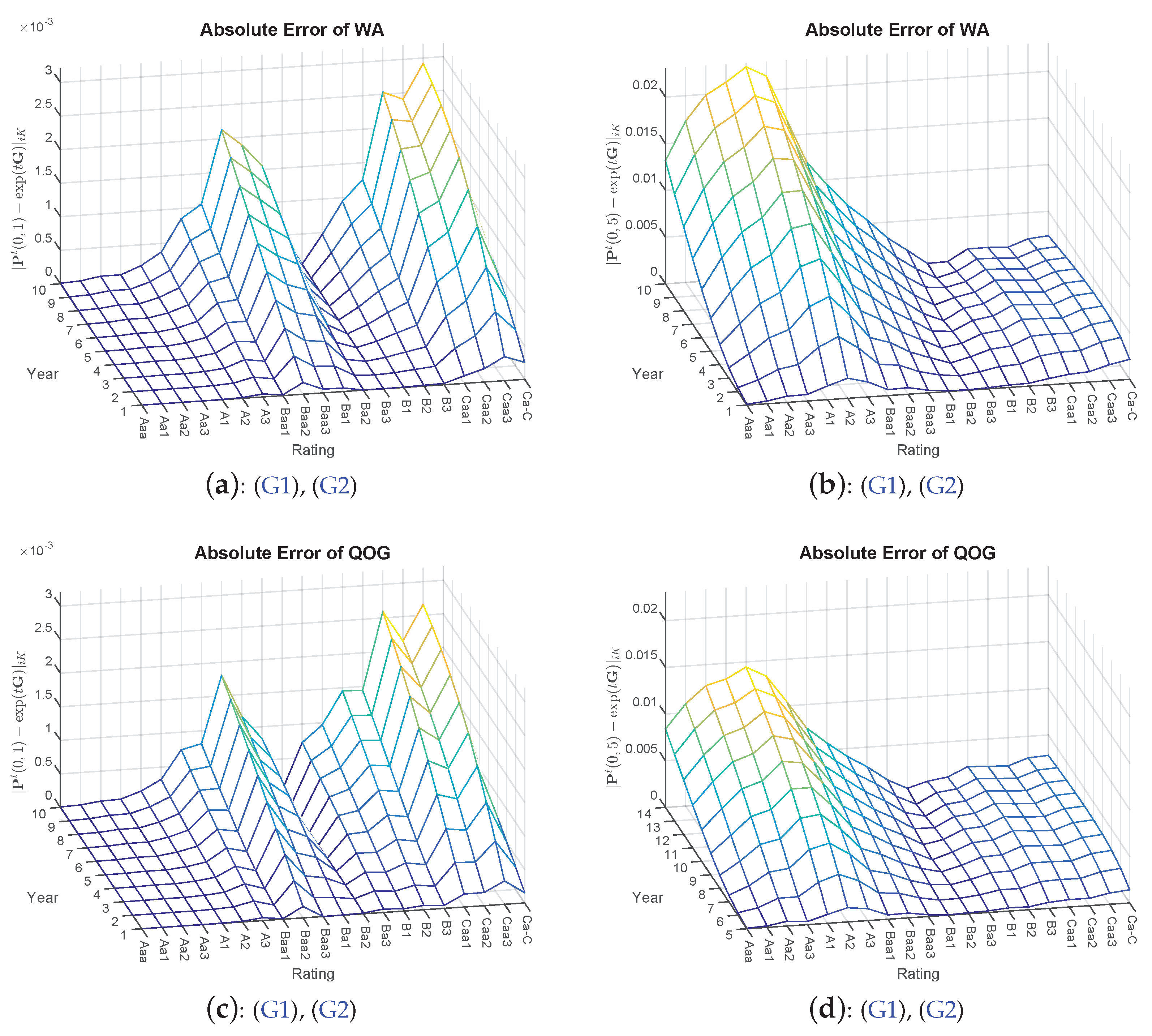
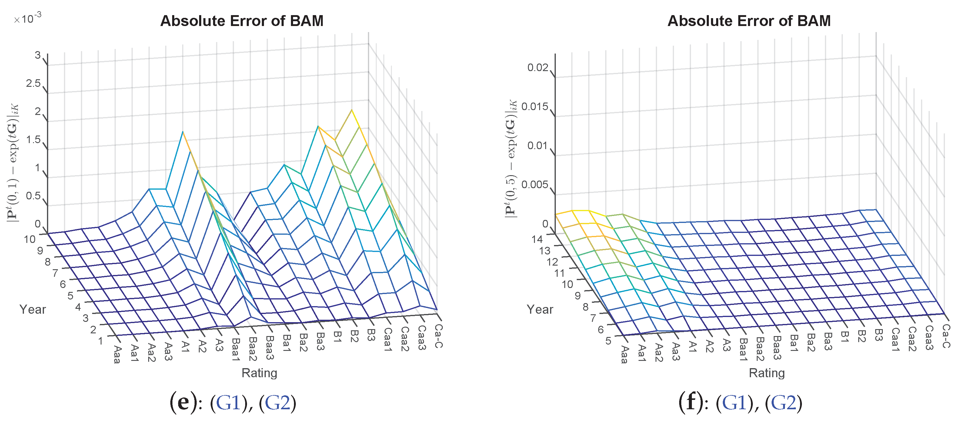
The results from Table 1 are further supported by taking a closer look at the default probabilities. Here, the absolute differences are compared with each other7. Therefore, in addition, we compute the future default probabilities of ten years. Visually, it can be inferred that a certain hierarchical order of the applied approaches can be observed in Figure 1, with QOG being superior to WA and BAM again being superior to QOG (and WA).
4.2. Towards Global Optimization
Global optimization approaches are introduced for potentially further improving the results from Section 4.1 benchmarked by BAM. Therefore, the following methods are applied:
- A homogenization approach is solved iteratively, where and the interval is discretized, for example, into steps of , thus moving from Problem 2 to Problem 1, where in each step, the start matrix is replaced by the optimal solution of the previous step. This way, a more robust procedure is obtained as the simpler (as convex problem) QOG is utilized for generating better start matrices, accordingly gaining accuracy in each iteration. More precisely, we find a generator matrix that, when exponentiated (by the matrix exponential), most closely matches the annual transition matrix , with:where denotes the Frobenius norm. Equivalently, as in Problems 2 and 1, the sets (Definition 4) and (Definition 5) can easily be included. Set (Definition 3), on the other hand, also needs to be homogenized, as well.
- Global solutions in combination with MATLAB’s local solver fmincon() with multiple start points.
- -
- ‘MultiStart’ (MS)
- -
- ‘GlobalSearch’ (GS)
Table 2 shows the results of the global optimization in comparison to BAM. No global technique is thereby superior to BAM; thus, the local solver is sufficient for obtaining a valid generator. From a computational perspective, it is also advisable to use BAM, as the durations are significantly shorter. Concluding, this outcome can also be interpreted as the confirmation of BAM delivering overall reliable results, although being a high-dimensional and nonlinear problem.
4.3. Constraints Analysis
We now extend the already conducted comparison of the default probabilities from Section 4.1 to the additional constraints. First of all, the averaged Frobenius norm of the complete resulting generator matrix is compared w.r.t. the optimization approaches with their corresponding constraints (Section 3). By adding the additional Constraints ((D1), (D2), (M1), (M2) and (R1)), the overall fit deteriorates as one deliberately moves away from the ‘true’ given transition matrix. Larger discrepancies are therefore to be expected when incorporating (M1) and (M2), as well as (R1), potentially effecting the whole matrix. Clearly, all additional constraints also depend on the state of the given transition matrix itself. Monotonically sorting w.r.t. migration probabilities, default probabilities and ratings and default probabilities larger or equal to 3 bp will have the same optimization result when only using (G1) and (G2). Overall better results can again be obtained with BAM as opposed to QOG. Similarly to Section 4.1, the improvement is smaller for the one-year transition matrices, while the difference in the distance decrease becomes more significant for the five-year forecast.
By increasing the constraints imposed to the optimization, the computation durations also increase. When looking at the two approaches more closely, the results show that for , BAM and QOG are approximately equally fast. For , BAM is consistently faster than QOG, while for , the opposite seems to be the case for some constraints. Albeit, the computations are overall in acceptable ranges from a modeling perspective, even for larger transition matrices. All results of the comparison based on the Frobenius norm and corresponding computation times can be viewed in Table 3.
Next, the impact of the additional constraints on the default probabilities is analyzed. Table 4 displays the post optimization default probabilities of the top four investment grade Classes Aaa, Aa, A and Baa of the transition matrix . Evidently, (D1) corrects and to 3 bp, and is affected by (D2), where the hierarchical order of ratings is restored. Subsequently, combining (D1) and (D2) will yield probabilities equal or larger to 3 bp. (M1) and (M2) do not show a major impact on the default probabilities, at least not on the higher ratings. However, a slight change can be registered compared to the (G1) and (G2) case. This may be attributed to the minor correction of being smaller than its right neighbor and, thus, also affecting the default probabilities to some extent. This will become more obvious when analyzing below. (R1), in turn, has a similar effect as (D2) with and . No major changes could be detected for Baa, all within a deviance of bp to the original probabilities at . Overall, the probabilities of BAM compared to QOG do resemble the original values of more accurately.
A visual depiction8 is given specifically of , as one can easily trace which constraint is responsible for its corresponding impact on the default probabilities. First, Constraint (D1) is added where in (a) and (b) of Figure 2, the ratings Aaa to A3 are adjusted to 3 bp. Not surprisingly, the errors grow accordingly, while all other rating classes remain unaffected (compare Figure 1c,e). Continuing with (c) and (d) of Figure 2, larger errors seem to occur for the rating Class Baa2. Indeed when looking at the matrix entry and its previous neighbor , it violates Constraint (D2). Thus, the post-optimization entry is then adjusted to causing higher errors. The effect of combining (D1) and (D2) can then be seen in (e) and (f), where the errors accumulate accordingly. A different picture than one may expect is presented in (g) and (h) of Figure 3, as (M1) and (M2) do not influence the default probabilities directly. Yet, we see a rise in discrepancy in rating Class Caa2.
For the following computations, we pretend that is a potential generator of the original given transition matrix for the sake of comparability of the pre- and post-optimization values. Indeed, , whereas , almost doubling the amount of its left neighbor, so that a larger correction is required for . This can be seen in Table 5, where for both optimizations QOG and BAM, the values are adjusted, so that is enforced. However, one can see that QOG already fails to maintain the original default probability of . In the long run, it is obvious that manipulated pre-default stages (here, Caa2 and Caa3) will then have an impact on the future default probabilities, which explains the offset in (g) and (h). Between Rows 17 and 18, several violations of (R1) can be detected. Exemplary for all, the largest discrepancy is picked with and . Table 6 shows that the original < (again, simply is computed of the original transition matrix), but is adjusted by QOG and BAM as required. Simultaneously, BAM can maintain the cumulative sum more closely to the original. The rectification of the rating Caa1 comes at a cost of loosing accuracy in the default probability. However, it can be observed (similarly to the (M1) and the (M2) case) that BAM is still closest to the original PDs. A summary of all effects can then be found in (k) and (l). Noteworthy is the positive effect when combining (M1) and (M2) with (R1), resulting in lower absolute errors in Caa1 compared to (R1) by itself.
5. Conclusions
Embedding a discrete transition matrix in continuous time is not an easy undertaking, as pre-conditions need to be met beforehand. The analysis of given annual transition matrices has revealed that it is often the case that theoretically, a valid generator does not exist, due to non-observed defaults in historical data for high rating classes. However, optimization problems can deal with this shortcoming and provide the closest solutions.
Three related optimization techniques have been considered in the literature. While QOG can be solved via a linear row-by-row approach, it has been shown that it can be solved similarly easily with additional linear constraints by linear programming. Analogous observations apply to BAM, which is the actual optimization problem of interest. The results are interesting for several reasons. Firstly, the non-convex and non-linear problem BAM is not only solvable, but, as expected, also yields (slightly) better results than QOG. Secondly, BAM has additionally gained more credibility of being the best optimal solution by introducing a robust homogenization approach.
The most noteworthy additional value however is the fact that credit risk-relevant constraints can be incorporated (and easily extended) into the optimization problems. It is up to the practitioner to decide which constraints are necessary or even additionally needed. In doing so, crude pre-manipulation of the transition matrix can be avoided, but instead be directly incorporated into the optimization, yielding a more elegant approach.
Acknowledgments
This research paper is part of the project regarding the modeling of the Pfandbriefe (German covered bonds), financially supported by the Bayerische Staatsministerium für Wissenschaft, Forschung und Kunst and backed by the corporate partners Allianz Deutschland AG, Deutsche Pfandbriefbank AG and DEVnet GmbH. Special thanks to Dirk Banholzer and Georg Schlüchtermann and participants of the annual OR2015 conference for their valuable input.
Author Contributions
The authors, Maximilian Hughes and Ralf Werner, contributed equally to this research paper.
Conflicts of Interest
The authors declare no conflict of interest.
Abbreviations
The following abbreviations are used in this manuscript:
| BAM | best approximation of the transition matrix |
| DA | diagonal adjustment |
| DMPG | distance minimization problem for the generator matrix |
| GS | global search |
| Homogen | homogenization |
| MCMC | Markov chain Monte Carlo |
| MS | multi-start |
| QOG | quasi-optimization of the generator |
| WA | weighted adjustment |
Appendix

| AAA | AA | A | BBB | BB | B | CCC-C | D | |
|---|---|---|---|---|---|---|---|---|
| AAA | 0.9193 | 0.0746 | 0.0048 | 0.0008 | 0.0004 | 0.0000 | 0.0000 | 0.0000 |
| AA | 0.0064 | 0.9180 | 0.0676 | 0.0060 | 0.0006 | 0.0011 | 0.0003 | 0.0000 |
| A | 0.0007 | 0.0227 | 0.9168 | 0.0512 | 0.0056 | 0.0025 | 0.0001 | 0.0004 |
| BBB | 0.0004 | 0.0027 | 0.0556 | 0.8789 | 0.0483 | 0.0102 | 0.0017 | 0.0023 |
| BB | 0.0004 | 0.0010 | 0.0061 | 0.0775 | 0.8148 | 0.0789 | 0.0111 | 0.0101 |
| B | 0.0000 | 0.0010 | 0.0028 | 0.0046 | 0.0695 | 0.8280 | 0.0396 | 0.0546 |
| CCC-C | 0.0019 | 0.0000 | 0.0037 | 0.0074 | 0.0243 | 0.1212 | 0.6046 | 0.2370 |
| D | 0.0000 | 0.0000 | 0.0000 | 0.0000 | 0.0000 | 0.0000 | 0.0000 | 1.0000 |
| Aaa | Aa | A | Baa | Ba | B | Caa-C | D | |
| Aaa | 0.8866 | 0.1030 | 0.0102 | 0.0000 | 0.0003 | 0.0000 | 0.0000 | 0.0000 |
| Aa | 0.0108 | 0.8870 | 0.0955 | 0.0034 | 0.0015 | 0.0015 | 0.0000 | 0.0003 |
| A | 0.0006 | 0.0288 | 0.9021 | 0.0592 | 0.0074 | 0.0018 | 0.0001 | 0.0001 |
| Baa | 0.0005 | 0.0034 | 0.0707 | 0.8523 | 0.0605 | 0.0101 | 0.0008 | 0.0016 |
| Ba | 0.0003 | 0.0008 | 0.0056 | 0.0568 | 0.8358 | 0.0808 | 0.0053 | 0.0146 |
| B | 0.0001 | 0.0004 | 0.0017 | 0.0065 | 0.0660 | 0.8270 | 0.0276 | 0.0706 |
| Caa-C | 0.0000 | 0.0000 | 0.0066 | 0.0105 | 0.0305 | 0.0611 | 0.6297 | 0.2616 |
| D | 0.0000 | 0.0000 | 0.0000 | 0.0000 | 0.0000 | 0.0000 | 0.0000 | 1.0000 |

| Aaa | Aa | A | Baa | Ba | B | Caa-C | D | |
|---|---|---|---|---|---|---|---|---|
| Aaa | −0.1212 | 0.1160 | 0.0051 | 0.0000 | 0.0001 | 0.0000 | 0.0000 | 0.0000 |
| Aa | 0.0121 | −0.1223 | 0.1069 | 0.0002 | 0.0012 | 0.0015 | 0.0000 | 0.0003 |
| A | 0.0005 | 0.0321 | −0.1075 | 0.0674 | 0.0061 | 0.0014 | 0.0000 | 0.0000 |
| Baa | 0.0006 | 0.0025 | 0.0805 | −0.1650 | 0.0713 | 0.0085 | 0.0008 | 0.0008 |
| Ba | 0.0003 | 0.0007 | 0.0036 | 0.0671 | −0.1857 | 0.0970 | 0.0054 | 0.0116 |
| B | 0.0001 | 0.0004 | 0.0014 | 0.0049 | 0.0787 | −0.1952 | 0.0380 | 0.0717 |
| Caa-C | 0.0000 | 0.0000 | 0.0080 | 0.0124 | 0.0380 | 0.0825 | −0.4644 | 0.3236 |
| D | 0.0000 | 0.0000 | 0.0000 | 0.0000 | 0.0000 | 0.0000 | 0.0000 | 0.0000 |
References
- A. Kreinin, and M. Sidelnikova. “Regularization Algorithms for Transition Matrices.” Algo Res. Q. 4 (2001): 23–40. [Google Scholar]
- E. Davies. “Embeddable Markov Matrices.” Electron. J. Probab. 15 (2010): 1474–1486. [Google Scholar] [CrossRef]
- W. Stromquist. Roots of Transition Matrices. Practical Paper; Exton, PA, USA: Daniel H. Wagner Associates, 1996. [Google Scholar]
- M. Araten, and L. Angbazo. Roots of Transition Matrices: Application to Settlement Risk. Practical Paper; New York, NY, USA: Chase Manhattan Bank (JPMorgan Chase & Co.), 1997. [Google Scholar]
- N.J. Higham, and L. Lin. “On pth Roots of Stochastic Matrices.” Linear Algebra Appl. 435 (2011): 448–463. [Google Scholar] [CrossRef]
- L. Lin. “Roots of Stochastic Matrices and Fractional Matrix Powers.” Ph.D. Thesis, University of Manchester, Manchester, UK, 2011. [Google Scholar]
- T. Charitos, P.R. de Waal, and L.C. van der Gaag. “Computing Short-Interval Transition Matrices of a Discrete-Time Markov Chain from Partially Observed Data.” Stat. Med. 27 (2008): 905–921. [Google Scholar] [CrossRef] [PubMed]
- Y. Inamura. Estimating Continuous Time Transition Matrices from Discretely Observed Data. Working Paper; Financial Systems and Bank Examination Department: Tokyo, Japan: Bank of Japan, 2006. [Google Scholar]
- J.R. Norris. Markov Chains. Number 2008 in Cambridge Series in Statistical and Probabilistic Mathematics; Cambridge, United Kingdom: Cambridge University Press, 1998. [Google Scholar]
- S. Asmussen. “Stochastic Modelling and Applied Probability.” In Applied Probability and Queues. New York, NY, USA: Springer, 2008. [Google Scholar]
- T. Bielecki, and M. Rutkowski. Credit Risk: Modeling, Valuation and Hedging. Berlin, Germany: Springer Finance; Springer, 2013. [Google Scholar]
- W.J. Culver. “On the Existence and Uniqueness of the Real Logarithm of a Matrix.” Proc. Am. Math. Soc. 17 (1966): 1146–1151. [Google Scholar] [CrossRef]
- B. Singer, and S. Spilerman. “The Representation of Social Processes by Markov Models.” Am. J. Sociol. 82 (1976): 1–54. [Google Scholar] [CrossRef]
- R.B. Israel, J.S. Rosenthal, and J.Z. Wei. “Finding Generators for Markov Chains via Empirical Transition Matrices, with Applications to Credit Ratings.” Math. Financ. 11 (2001): 245–265. [Google Scholar] [CrossRef]
- G. Elfving. “Zur Theorie der Markoffschen Ketten.” Acta Soc. Sci. Fenn. 8 (1937): 1–17. [Google Scholar]
- J.F.C. Kingman. “The Imbedding Problem for Finite Markov Chains.” Z. Wahrscheinlichkeitstheorie Verwandte Geb. 1 (1962): 14–24. [Google Scholar] [CrossRef]
- M.A. Guerry. “On the Embedding Problem for Discrete-Time Markov Chains.” J. Appl. Probab. 50 (2013): 918–930. [Google Scholar] [CrossRef]
- J. Cuthbert. “The Logarithmic Function for Finite-State Markov Semi-Groups.” J. Lond. Math. Soc. 6 (1973): 524–532. [Google Scholar] [CrossRef]
- S. Johansen. “Some Results on the Imbedding Problem for Finite Markov Chains.” J. Lond. Math. Soc. 2 (1974): 345–351. [Google Scholar] [CrossRef]
- H. Frydman. “The Embedding Problem for Markov Chains with Three States.” Math. Proc. Camb. Philos. Soc. 87 (1980): 285–294. [Google Scholar] [CrossRef]
- P. Carette. “Characterizations of Embeddable 3 × 3 Stochastic Matrices with a Negative Eigenvalue.” N. Y. J. Math. 1 (1995): 120–129. [Google Scholar]
- M.A. Guerry. “On the Embedding Problem for Three-State Markov Chains.” In Proceedings of the World Congress on Engineering 2014, London, UK, 2–4 July 2014; Volume II.
- K. Chung. Markov Chains with Stationary Transition Probabilities. Die Grundlehren der mathematischen Wissenschaften; Berlin, Germany: Springer, 1960. [Google Scholar]
- G. Grimmett, and D. Stirzaker. “Probability and random processes.” In Probability and Random Processes. Oxford, UK: OUP Oxford, 2001. [Google Scholar]
- G.S. Goodman. “An Intrinsic Time for Non-Stationary Finite Markov Chains.” Z. Wahrscheinlichkeitstheorie Verwandte Geb. 16 (1970): 165–180. [Google Scholar] [CrossRef]
- R.A. Jarrow, D. Lando, and S.M. Turnbull. “A Markov Model for the Term Structure of Credit Risk Spreads.” Rev. Financ. Stud. 10 (1997): 481–523. [Google Scholar] [CrossRef]
- W. Anderson. Continuous-Time Markov Chains: An Applications-Oriented Approach. New York, NY, USA: Springer, 2012. [Google Scholar]
- A. Metz, and R. Cantor. “Moody’s Credit Policy—Introducing Moody’s Credit Transition Model.” Available online: http://www.moodysanalytics.com/ /media/Brochures/Credit-Research-Risk-Measurement/Quantative-Insight/Credit-Transition-Model/Introductory-Article-Credit-Transition-Model.pdf (accessed on 29 August 2016).
Figure 1.
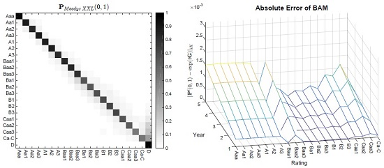
Absolute errors of the methods WA, QOG and BAM (QOG and BAM optimizations based on Constraints (G1) and (G2)) with starting point . Left side: (a, c,e) transition matrix ; right side: (b,d,f) transition matrix .
Figure 1.
Absolute errors of the methods WA, QOG and BAM (QOG and BAM optimizations based on Constraints (G1) and (G2)) with starting point . Left side: (a, c,e) transition matrix ; right side: (b,d,f) transition matrix .


Figure 2.
Absolute errors of Problems QOG and BAM based on various additional constraints with starting point , for transition matrix in Table A1. Left side: (a,c,e) QOG; right side: (b,d,f) BAM.
Figure 2.
Absolute errors of Problems QOG and BAM based on various additional constraints with starting point , for transition matrix in Table A1. Left side: (a,c,e) QOG; right side: (b,d,f) BAM.
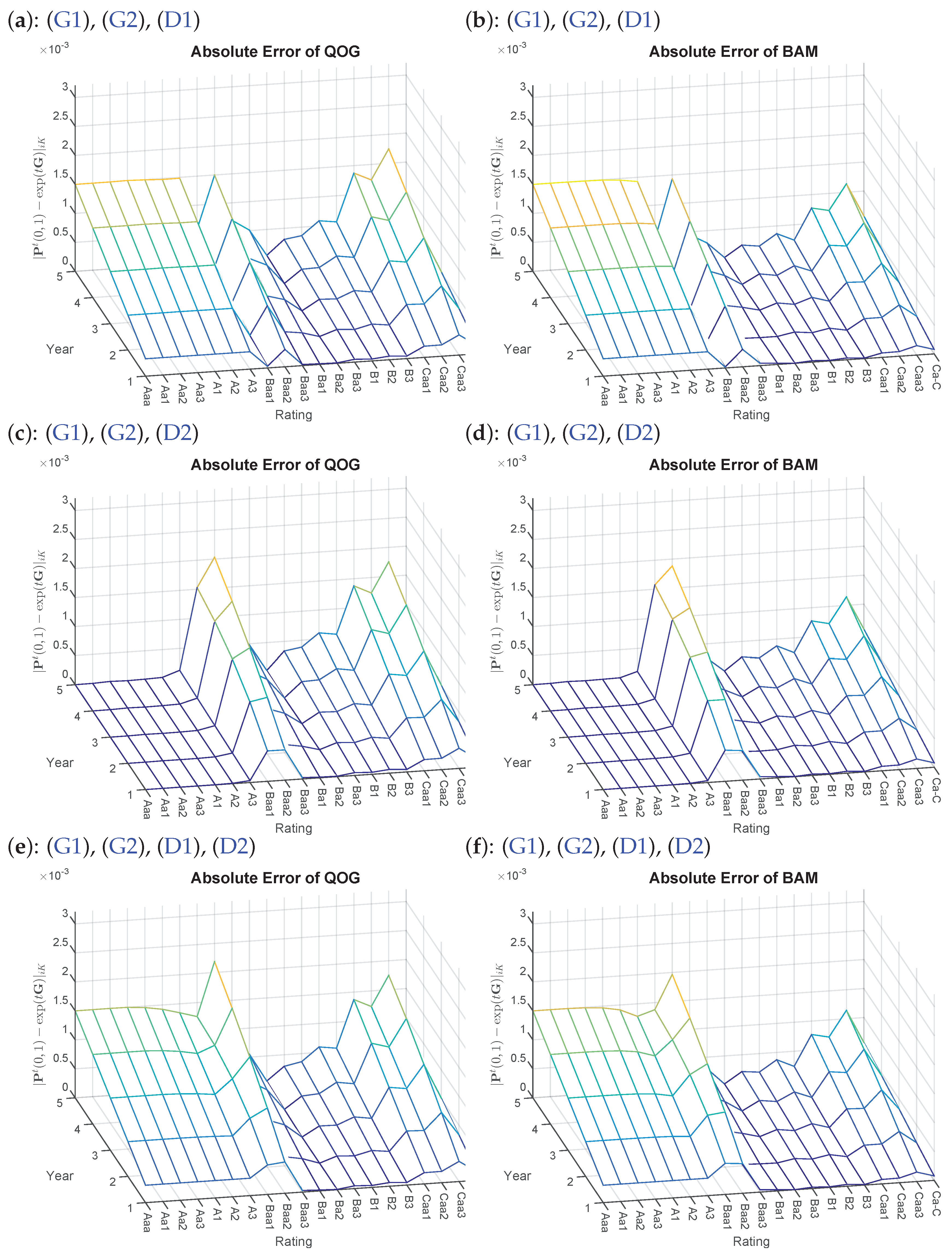
Figure 3.
Absolute errors of Problems QOG and BAM based on various additional constraints with starting point , for transition matrix in Table A1. Left side: (g,i,k) QOG; right side: (h,j,l) BAM.
Figure 3.
Absolute errors of Problems QOG and BAM based on various additional constraints with starting point , for transition matrix in Table A1. Left side: (g,i,k) QOG; right side: (h,j,l) BAM.
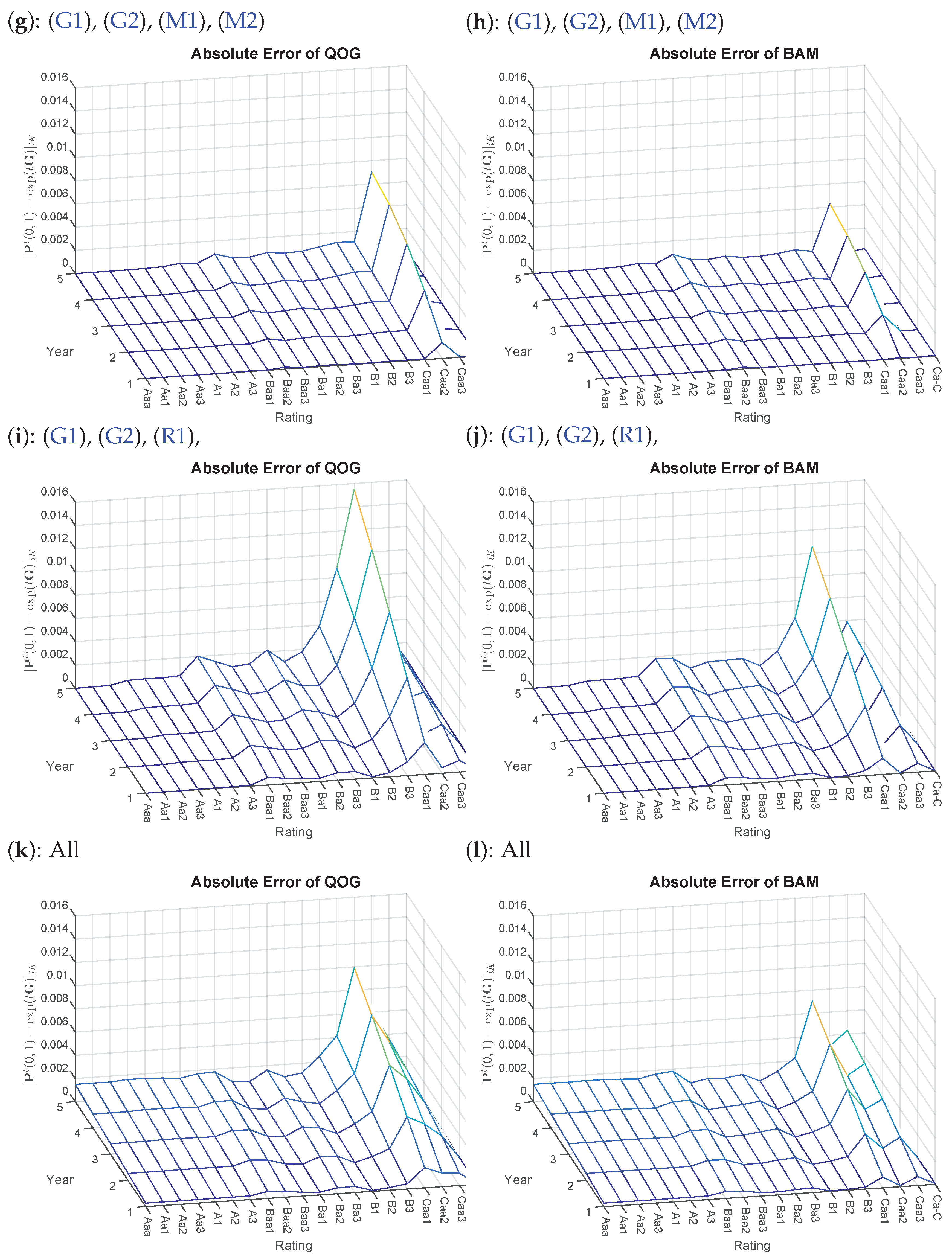
Table 1.
Comparison of the regularization methods based on averaged Frobenius norm (QOG and BAM optimizations based on Constraints (G1) and (G2)), for given transition matrices from Moodys in Table A1.
| Constraints | Method | Start Matrix | |||
|---|---|---|---|---|---|
| (G1), (G2) | DA | ||||
| WA | |||||
| DMPG | |||||
| QOG | |||||
| (0.21 s) | (7.18 s) | (10.70 s) | |||
| (0.38 s) | (9.91 s) | (21.06 s) | |||
| (0.14 s) | (4.02 s) | (4.60 s) | |||
| BAM | |||||
| (0.16 s) | (1.92 s) | (17.33 s) | |||
| (0.17 s) | (2.22 s) | (27.07 s) | |||
| (0.16 s) | (3.41 s) | (18.26 s) | |||
| (0.20 s) | (4.24 s) | (23.72 s) |
Table 2.
Comparison of global solutions based on the averaged Frobenius norm and Constraints (G1), (G2) with starting point , for given transition matrices from Moodys in Table A1 (* the MS method uses a set of 100 different start points, which are parallelized).
| Constraints | Method | |||
|---|---|---|---|---|
| (G1), (G2) | Homogen | |||
| (24.95 s) | (718.74 s) | (1938.16 s) | ||
| MS | ||||
| (32.67 s) | (1353.93 s) | (12509.95 s) | ||
| GS | ||||
| (2.77 s) | (18.01 s) | (9447.82 s) |
Table 3.
Comparison of the additional constraints of QOG and BAM based on the averaged Frobenius norm with starting point , for given transition matrices from Moodys in Table A1.
| Constraints | Method | |||
|---|---|---|---|---|
| (G1), (G2), (D1) | QOG | |||
| (0.62 s) | (11.13 s) | (22.70 s) | ||
| BAM | ||||
| (0.31 s) | (3.31 s) | (26.25 s) | ||
| (G1), (G2), (D2) | QOG | |||
| (0.66 s) | (18.21 s) | (4.65 s) | ||
| BAM | ||||
| (0.31 s) | (6.32 s) | (26.36 s) | ||
| (G1), (G2), (D1), (D2) | QOG | |||
| (0.49 s) | (16.07 s) | (22.44 s) | ||
| BAM | ||||
| (0.31 s) | (3.93 s) | (27.44 s) | ||
| (G1), (G2), (M1), (M2) | QOG | |||
| (0.22 s) | (13.97 s) | (22.26 s) | ||
| BAM | ||||
| (0.28 s) | (5.46 s) | (114.72 s) | ||
| (G1), (G2), (R1) | QOG | |||
| (0.42 s) | (14.91 s) | (78.80 s) | ||
| BAM | ||||
| (0.33 s) | (4.30 s) | (32.88 s) | ||
| All | QOG | |||
| (0.42 s) | (15.95 s) | (38.06 s) | ||
| BAM | ||||
| (0.51 s) | (6.41 s) | (51.18 s) |
Table 4.
Comparison of one- and five-year default probabilities in the basis points (bp) of QOG and BAM, for given transition matrix in Table A1.
| One Year () | Five Year () | ||||||||
|---|---|---|---|---|---|---|---|---|---|
| Constraints | Method | Aaa | Aa | A | Baa | Aaa | Aa | A | Baa |
| Original | 0.00 | 3.11 | 1.04 | 15.87 | 5.01 | 28.85 | 47.69 | 231.67 | |
| (G1), (D2) | QOG | 0.17 | 3.12 | 1.42 | 15.89 | 6.35 | 29.69 | 49.17 | 231.92 |
| BAM | 0.17 | 3.05 | 1.40 | 15.86 | 6.20 | 29.32 | 48.94 | 231.82 | |
| (G1), (G2), (D1) | QOG | 3.00 | 3.49 | 3.00 | 16.01 | 18.04 | 32.56 | 55.81 | 233.29 |
| BAM | 3.00 | 3.12 | 3.00 | 15.87 | 17.65 | 30.99 | 55.19 | 232.73 | |
| (G1), (G2), (D2) | QOG | 0.12 | 2.08 | 2.08 | 15.95 | 5.39 | 26.11 | 51.73 | 232.46 |
| BAM | 0.12 | 2.06 | 2.06 | 15.87 | 5.29 | 25.96 | 51.35 | 232.17 | |
| (G1), (G2), (D1), (D2) | QOG | 3.00 | 3.00 | 3.00 | 16.01 | 17.65 | 30.66 | 55.70 | 233.26 |
| BAM | 3.00 | 3.00 | 3.00 | 15.87 | 17.55 | 30.52 | 55.16 | 232.73 | |
| (G1), (G2), (M1), (M2) | QOG | 0.16 | 2.93 | 1.41 | 15.89 | 5.36 | 25.88 | 48.97 | 231.88 |
| BAM | 0.17 | 3.08 | 1.41 | 15.86 | 5.52 | 26.51 | 49.06 | 231.82 | |
| (G1), (G2), (R1) | QOG | 0.07 | 1.28 | 1.99 | 15.09 | 4.36 | 21.77 | 49.44 | 222.44 |
| BAM | 0.08 | 1.47 | 2.19 | 15.57 | 4.59 | 22.98 | 51.09 | 227.43 | |
| All | QOG | 3.00 | 3.41 | 4.08 | 15.17 | 17.41 | 29.36 | 56.96 | 223.86 |
| BAM | 3.00 | 3.42 | 4.12 | 15.50 | 17.46 | 29.70 | 58.22 | 228.29 | |
Table 5.
Corrections of the additional Constraints (M1) and (M2) and their impact on the default probabilities of QOG and BAM, for transition matrix in Table A1.
| Constraints | Method | |||
|---|---|---|---|---|
| (G1), (G2), (M1), (M2) | Original | 0.0440 | 0.0838 | 0.1735 |
| QOG | 0.0638 | 0.0638 | 0.1721 | |
| BAM | 0.0641 | 0.0641 | 0.1734 |
Table 6.
Corrections of the additional Constraint (R1) and its impact on the default probabilities of QOG and BAM, for transition matrix in Table A1.
| Constraints | Method | |||
|---|---|---|---|---|
| (G1), (G2), (R1) | Original | −0.0059 | −0.0173 | 0.0931 |
| QOG | −0.0189 | −0.0189 | 0.0904 | |
| BAM | −0.0163 | −0.0163 | 0.0917 |
- 2.Version 8.4.0 (R2014b), The MathWorks Inc., Natick, MA, USA.
- 3.We distinguish between general transition matrices in theory, denoted by , and given transition matrices by rating agencies, denoted by , if not stated otherwise.
- 4.Each single additional constraint can be switched on or off according to the user’s preferences. Further extensions are conceivable.
- 5.As can be seen on the right picture of Table A1, the majority of probability mass for lower ratings is shifted from the main diagonal to the default column, revealing a rather atypical transition matrix.
- 6.The principal logarithm of has the nearest negative off-diagonal entry to zero. This also applies to .
- 7.DA and DMPG are deliberately omitted at this point due to the results in Table 1. Furthermore, the visual depiction of is spared due to too small differences.
- 8.Again, is omitted, yielding too close results where detecting differences visually is not feasible. Furthermore, is not included, as some of the probability mass has already migrated to the default state; thus, visually, there is not much insight to gain.
© 2016 by the authors; licensee MDPI, Basel, Switzerland. This article is an open access article distributed under the terms and conditions of the Creative Commons Attribution (CC-BY) license (http://creativecommons.org/licenses/by/4.0/).
Share and Cite
MDPI and ACS Style
Hughes, M.; Werner, R. Choosing Markovian Credit Migration Matrices by Nonlinear Optimization. Risks 2016, 4, 31. https://doi.org/10.3390/risks4030031
AMA Style
Hughes M, Werner R. Choosing Markovian Credit Migration Matrices by Nonlinear Optimization. Risks. 2016; 4(3):31. https://doi.org/10.3390/risks4030031
Chicago/Turabian StyleHughes, Maximilian, and Ralf Werner. 2016. "Choosing Markovian Credit Migration Matrices by Nonlinear Optimization" Risks 4, no. 3: 31. https://doi.org/10.3390/risks4030031
Note that from the first issue of 2016, this journal uses article numbers instead of page numbers. See further details here.