Multivariate TVaR-Based Risk Decomposition for Vector-Valued Portfolios

Abstract

In order to protect stakeholders of insurance companies and financial institutions against adverse outcomes of risky businesses, regulators and senior management use capital allocation techniques. For enterprise-wide risk management, it has become important to calculate the contribution of each risk within a portfolio. For that purpose, bivariate lower and upper orthant tail value-at-risk can be used for capital allocation. In this paper, we present multivariate value-at-risk and tail-value-at-risk for $d\ge 2$, and we focus on three different methods to calculate optimal values for the contribution of each risk within the sums of random vectors to the overall portfolio, which could particularly apply to insurance and financial portfolios.

1. Introduction

For insurance companies and financial institutions, regulations are established for solvency capital requirements. Internal targets and supervisory requirements are in constant evolution, following the progress in measurement techniques. For example, since recent financial events, regulators aim at protecting stakeholders against large unexpected losses using conservative measures. In this paper, we provide new ways to compute the contribution of each component of a portfolio composed of dependent classes of risks. We consider multivariate risk measures, represented by sets of curves, that can be used for risk comparison. We also provide methods to select optimal sets from these curves, in order to obtain vector-valued sets the same dimension as the total number of risks. Our approach allows a conservative risk protection, which is in line with desirable changes, as a consequence of the recent financial crisis and catastrophic events. Sherris [1] studies how to distribute the expected policyholder deficit to each business line under a complete market condition. Kim and Hardy [2] study the allocation principle on policyholders’ deficit. In this paper, we calculate the capital allocation for each class, following optimal capital allocation principles as presented in Dhaene et al. [3], which consider diversification within each line of business, presented as the unified principle in Dhaene et al. [4]. We calculate the contribution for each risk within a business unit using the top-down risk decomposition technique (see, e.g., Cossette et al. [5]), based on multivariate risk measures. Therefore, our approach considers both the dependence between each risk within a class and the dependence between classes of risks.

For univariate random variables representing aggregate portfolios, Value-at-Risk (VaR) and Tail Value-at-Risk (TVaR), are useful tools that fulfil desirable risk measure properties when one studies tail distributions. For instance, the univariate VaR provides a quantile at a determined probability level and is always homogeneous, invariant in translation and monotonic. The TVaR has the advantage of providing information on the tail of the distribution and is always coherent, unlike the VaR. Note that TVaR and Conditional Tail Expectation (CTE) are equal for continuous random variables. We choose to work with TVaR, since CTE is not coherent for discrete random variables. In this paper, we do not use univariate risk decomposition techniques, since we consider portfolios where groups of homogeneous risks are heterogeneous and cannot be aggregated. We choose to base the risk decomposition on multivariate TVaR and focus on continuous random variables. As stated in Aziz and Rosen [6], the aggregation of risks is still at an early stage, and for historical and business reasons, one might want more conservative methods, to ensure every business line to be covered up to a chosen level. For example, conglomerates cannot use dedicated capital from business operations to mitigate other risks. The Basel Committee on Banking Supervision (BCBS) and the Office of the Superintendent of Financial Institutions (OSFI) have also published discussions on the risks concerning aggregation techniques for capital allocation (e.g., BCBS [7], BCBS [8] and OSFI [9]) and suggest considering capital allocation to protect every unique branch of activities to a defined level, instead of their aggregation, which is exactly in line with the multivariate TVaR-based risk decomposition technique presented in this paper. Under the terms of Basel and OSFI Own Risk and Solvency Assessment (ORSA), banks and insurance companies often measure the risk associated with a portfolio $X=(X_1,\cdots ,X_n)$ in terms of ${\mathrm{VaR}}_{\alpha }(X_1+\cdots +X_n)$, ${\mathrm{TVaR}}_{\alpha }(X_1+\cdots +X_n)$, the risk measure being calculated for the sum of its marginal components. This is for example the case for operational risk; see Embrechts and Puccetti [10]. However, OSFI [11] states that “No diversification between risk categories is permitted until evidence confirms diversification will hold in a stress situation”. In this paper, we suggest the multivariate TVaR-based risk decomposition technique to consider that there might be heterogeneous risks or risks that cannot be diversified by their aggregation. The contribution of each risk is expressed in terms of a curve. Then, we present three different methods to select specific sets from the curves, which can be useful for practical purposes. The latter situation legitimates the use of multivariate risk measures on which to base capital allocation, as presented in the next sections. See Cossette et al. ( [12,13]) for a review of multivariate risk measures.

We denote the truncated expectation of X, truncated from below at b, by $\mathbb{E}\left[X\times 1_{\left\{X>b\right\}}\right]$, where $1_A$ is the indicator function, such that $1_A\left(X\right)=1$, if $X\in A$, and $1_A\left(X\right)=0$, if $X\notin A$. Then, as introduced in Acerbi and Tasche [14], for $S={\sum }_{i=1}^n{X}_i$, the univariate TVaR of X at level α, $0\le \alpha <1$,

$$\begin{array}{ccc}\hfill {\mathrm{TVaR}}_{\alpha }\left(S\right)& =& \frac{1}{1-\alpha }{\int }_{\alpha }^1{\mathrm{VaR}}_u\left(S\right)du\hfill \\ & =& \frac{E\left[S\times 1_{\left\{S>{\mathrm{VaR}}_{\alpha }\left(S\right)\right\}}\right]+{\mathrm{VaR}}_{\alpha }\left(S\right)\left(F_S\left({\mathrm{VaR}}_{\alpha }\left(S\right)\right)-\alpha \right)}{1-\alpha }\hfill \\ & =& \frac{E\left[S\right]-E\left[S\times 1_{\left\{S\le {\mathrm{VaR}}_{\alpha }\left(S\right)\right\}}\right]+{\mathrm{VaR}}_{\alpha }\left(S\right)\left(F_S\left({\mathrm{VaR}}_{\alpha }\left(S\right)\right)-\alpha \right)}{1-\alpha },\hfill \end{array}$$

where:

$${\mathrm{VaR}}_{\alpha }\left(S\right)=inf\left\{s\in \mathbb{R},F_S\left(s\right)\ge \alpha \right\}.$$

Insurance and reinsurance companies take responsibility not only to allocate capital for a portfolio, but most of the time, also to its individual components. This consideration is also useful for pricing and comparison purposes. Furthermore, the computation of the contributions of each risk to the overall portfolio allows the identification of riskier assets or classes of risks and to prevent from catastrophic events, in addition to fulfilling regulation requirements. Capital allocation techniques are mostly split into two different approaches. A top-down approach is presented in Tasche [15], Panjer [16] and Goovaerts et al. [17], where the capital is first allocated to the aggregate portfolio and then split into its internal business lines, using different techniques. The other general method consists of optimization functions, as in Dhaene et al. [3] and Kim and Hardy [2]. It is desirable to share equitably the risk capital between the portfolio’s risky components, considering their dependence level. In this paper, we will focus on the top-down risk decomposition technique.

However, aggregating a portfolio implies that if a risk reaches a high probability level, the other risks will compensate, to preserve a portfolio risk level. This is still being considered and accepted by recent regulatory frameworks and guidelines, but only within each line of business. For cases where business units aggregation is not an option, multivariate risk measures are used to allocate capital for components or classes of aggregate risks of the overall portfolio. This conservative allocation reflects the uncertainty of our economy and attempts to find a balance between making expected losses and preserving capital for the extreme events. For example, we find its purpose for an insurance company with multivariate business lines, represented as follows:

$$\begin{array}{c}\begin{array}{ccc}\mathrm{Business}\mathrm{line}1& \dots & \mathrm{Business}\mathrm{line}k\end{array}\hfill \\ \begin{array}{c}\left(\begin{array}{ccc}\left[\begin{array}{c}{X}_{1,1}\\ ⋮\\ X_{1,n}\end{array}\right]& ,\dots ,& \left[\begin{array}{c}{X}_{k,1}\\ ⋮\\ X_{k,n}\end{array}\right]\end{array}\right)\end{array}\begin{array}{c}\to \mathrm{Policy}1\\ ⋮\\ \to \mathrm{Policy}n.\end{array}\hfill \end{array}$$

From an insurance point of view, business lines can represent the capital allocated for losses and dependent allocation expenses, and the policies are the insureds. From a financial point of view, business lines can be interpreted as portfolios, and the policies would represent dependent positions. This framework is also considered in Izraylevich and Tsudikman [18].

In Section 2, desirable properties of risk contributions are set, the univariate TVaR-based allocation principle is described and multivariate extensions, lower and upper orthant VaR and TVaR, discussed in Cossette et al. ( [12,13]), are presented. Section 3 defines lower and upper orthant risk decomposition methods for each risk and group of aggregated risks. We also present the multivariate extension of desirable properties for risk decomposition in a multivariate setting. In Section 4, we select sets using optimization functions, in order to calculate the risk decomposition sets. Three different techniques to select allocation sets from the curves resulting from the contributions are presented. Section 5 contains illustrative applications of our results. They illustrate different values obtained when changing the dependence structures within and between the lines of business of a portfolio composed of two aggregate classes.

2. Preliminaries

In this section, we introduce basic notions and useful notation for the continuation.

2.1. Desirable Properties of Contributions

Let us first recall the properties for coherent allocation, based on univariate risk measures, as suggested in Denault [19] and Kalkbrener [20]. Let $X_1,\cdots ,X_n$ be a sequence of risks, and put $S=X_1+\cdots +X_n$. Consider a univariate risk measure $\rho \left(S\right)$ and the contribution function $\rho (X_i;S)$ that satisfies $\rho (S;S)=\rho \left(S\right)$. One wishes to fulfil the following axioms.

A1. Full allocation:

The capital allocation for the overall portfolio is split into all of its sub-portfolios, that is:

$$\rho (a_1{X}_1+\cdots +a_n{X}_n)=\sum _{i=1}^n{a}_i\rho (X_i;S),a_i\in \mathbb{R}.$$

In particular, the capital allocated to the aggregate portfolio is entirely split into its components. Indeed, for $a_i=1$, $i=1,\cdots ,n$, one has:

$$\rho \left(S\right)=\sum _{i=1}^n\rho (X_i;S).$$

A2. No undercut:

For any subset (decomposition of the total risk) $T\subset \{1,\cdots ,n\}$,

$$\sum _{i\in T}\rho (X_i;S)\le \rho \left(\sum _{i\in T}{X}_i;S\right).$$

No portfolio can undercut the proposed allocation, that is an undercut occurs when a portfolio’s allocation is higher than the amount of risk capital it would face as an entity separate from the firm.

A3. Diversification:

Each contribution does not exceed the value of capital allocated to this risk, considered as a stand-alone portfolio:

$$\rho (X_i;S)\le \rho (X_i;X_i)=\rho \left(X_i\right).$$

A4. Symmetry:

The substitution of one risk $X_i$ by another identical risk $X_j$ will result in no change in the allocations, that is,

$$\rho (X_i;S)=\rho (X_j;S),i\ne j.$$

This axiom ensures that a portfolio’s allocation depends only on its contribution to risk within the firm, no matter how the overall remaining portfolio is constituted.

A5. Consistency:

For any scalar $k\in \mathbb{R}$, $\rho \left(k\right)=k$. This means that, all other things being equal, the capital allocated to a risk that has no uncertainty should not affect the initial cash position.

A6. Continuity:

Small changes to the portfolio only have a limited effect on the risk capital of its sub-portfolios.

$$\underset{ϵ\to 0}{lim}\rho (X_i;S+ϵX_i)=\rho (X_i;S).$$

2.2. Univariate TVaR-Based Allocation Rule

For an aggregate portfolio of continuous risks, based on the univariate TVaR risk measure, the contributions of each risk are obtained by the following:

$${\mathrm{TVaR}}_{\alpha }(X_i;S)=\frac{1}{1-\alpha }\mathbb{E}\left[X_i{1}_{\left\{S>{\mathrm{VaR}}_{\alpha }\left(S\right)\right\}}\right].$$

(1)

This allocation method fulfils the desirable properties stated in Section 2.1.

It can be easily shown that the sum of TVaR contributions is equal to the TVaR of the aggregate claim amount, i.e.,

$${\mathrm{TVaR}}_{\alpha }\left(S\right)=\sum _{i=1}^n{\mathrm{TVaR}}_{\alpha }(X_i;S).$$

We refer the reader to McNeil et al. [21] for more details on the TVaR-based allocation rule.

2.3. Multivariate Lower and Upper Orthant TVaR

In Cossette et al. [12], definitions of the lower and upper orthant VaR, in the bivariate case, are provided. These definitions can be extended to a multivariate setting. To this end, let $\mathbf{X}=(X_1,\cdots ,X_n)$ be a random vector with continuous cumulative distribution function (cdf) F and survival function $\overline{F}$. For $\mathbf{x}=(x_1,\cdots ,x_n)\in {\mathbb{R}}^n$, denote ${\mathbf{x}}_{\backslash i}=(x_1,\cdots ,x_{i-1},x_{i+1},\cdots ,x_n)$. For fixed ${\mathbf{x}}_{\backslash i}$, define the functions $F_{{\mathbf{x}}_{\backslash i}}:x_i\to F\left(\mathbf{x}\right)$ and ${\overline{F}}_{{\mathbf{x}}_{\backslash i}}:x_i\to \overline{F}\left(\mathbf{x}\right)$. The components of multivariate lower and upper orthant VaR at level α are then defined as the inverse of the function $F_{{\mathbf{x}}_{\backslash i}}$ and ${\overline{F}}_{{\mathbf{x}}_{\backslash i}}$ at α and $1-\alpha$, respectively. Then, the components of the multivariate lower and upper orthant VaRs are represented by:

$${\underline{\mathrm{VaR}}}_{{}_{\alpha ,{\mathbf{x}}_{\backslash i}}}\left(\mathbf{X}\right)=F_{{\mathbf{x}}_{\backslash i}}^{-1}\left(\alpha \right)\mathrm{and}{\overline{\mathrm{VaR}}}_{{}_{\alpha ,{\mathbf{x}}_{\backslash i}}}\left(\mathbf{X}\right)={\overline{F}}_{{\mathbf{x}}_{\backslash i}}^{-1}(1-\alpha ),i=1,\cdots ,n.$$

The multivariate lower and upper orthant VaRs at level α are given by:

$${\underline{\mathrm{VaR}}}_{\alpha ,\mathbf{x}}\left(\mathbf{X}\right)=\left({\underline{\mathrm{VaR}}}_{{}_{\alpha ,{\mathbf{x}}_{\backslash 1}}}\left(\mathbf{X}\right),\cdots ,{\underline{\mathrm{VaR}}}_{{}_{\alpha ,{\mathbf{x}}_{\backslash n}}}\left(\mathbf{X}\right)\right),$$

and:

$${\overline{\mathrm{VaR}}}_{\alpha ,\mathbf{x}}\left(\mathbf{X}\right)=\left({\overline{\mathrm{VaR}}}_{{}_{\alpha ,{\mathbf{x}}_{\backslash 1}}}\left(\mathbf{X}\right),\cdots ,{\overline{\mathrm{VaR}}}_{{}_{\alpha ,{\mathbf{x}}_{\backslash n}}}\left(\mathbf{X}\right)\right),$$

respectively. Let $F_{\backslash i}$ and ${\overline{F}}_{\backslash i}$ be the distribution and survival function of the random vector ${\mathbf{X}}_{\backslash i}=(X_1,\cdots ,X_{i-1},X_{i+1},\cdots ,X_n)$. These distributions take into consideration all of the random variables on which $X_i$ depends when calculating the joint distribution function and survival function at level α for $X_i$, therefore incorporating the dependence in the calculation of the risk measure. We observe that ${\underline{\mathrm{VaR}}}_{\alpha ,{\mathbf{x}}_{\backslash i}}\left(\mathbf{X}\right)$ represents the VaR of the conditional random variable $X_i|{\mathbf{X}}_{\backslash i}\le {\mathbf{x}}_{\backslash i}$ at level $\frac{\alpha }{F_{\backslash i}\left({\mathbf{x}}_{\backslash i}\right)}$. Furthermore, ${\overline{\mathrm{VaR}}}_{\alpha ,{\mathbf{x}}_{\backslash i}}\left(\mathbf{X}\right)$ is the VaR of the conditional random variable $X_i|{\mathbf{X}}_i\ge {\mathbf{x}}_i$ at level $\frac{\alpha -F_{\backslash i}\left({\mathbf{x}}_{\backslash i}\right)}{{\overline{F}}_{\backslash i}\left({\mathbf{x}}_{\backslash i}\right)}$.

The multivariate lower orthant VaR can be interpreted as the threshold that ensures each set of random variables to be protected at level α, so that sets above this curve would be considered as being tail events. The multivariate upper orthant VaR can be interpreted as being the curve above which events provide a smaller joint survival probability.

Definition 1.

Consider $\mathbf{X}$ to be continuous. The multivariate lower and upper orthant TVaR are defined as follows.

(i) 

For all ${\mathbf{x}}_{\backslash i}\ge (F_{X_1}^{-1}\left(\alpha \right),\cdots ,F_{X_{i-1}}^{-1}\left(\alpha \right),F_{X_{i+1}}^{-1}\left(\alpha \right),\cdots ,F_{X_k}^{-1}\left(\alpha \right))$, one has:

$$\begin{array}{ccc}\hfill {\underline{TVaR}}_{{}_{\alpha ,{\mathbf{x}}_{\backslash i}}}\left(\mathbf{X}\right)& =& \mathbb{E}[X_i|X_i>{\underline{VaR}}_{{}_{\alpha ,{\mathbf{x}}_{\backslash i}}}\left(\mathbf{X}\right),{\mathbf{X}}_{\backslash i}\le {\mathbf{x}}_{\backslash i}]\hfill \\ & =& \frac{1}{F_{\backslash i}\left({\mathbf{x}}_{\backslash i}\right)-\alpha }{\int }_{\alpha }^{F_{\backslash i}\left({\mathbf{x}}_{\backslash i}\right)}{\underline{VaR}}_{u,{\mathbf{x}}_{\backslash i}}\left(\mathbf{X}\right)du.\hfill \end{array}$$

(ii) 

For all ${\mathbf{x}}_{\backslash i}\le (F_{X_1}^{-1}\left(\alpha \right),\cdots ,F_{X_{i-1}}^{-1}\left(\alpha \right),F_{X_{i+1}}^{-1}\left(\alpha \right),\cdots ,F_{X_k}^{-1}\left(\alpha \right))$, one has:

$$\begin{array}{ccc}\hfill {\overline{TVaR}}_{{}_{\alpha ,{\mathbf{x}}_{\backslash i}}}\left(\mathbf{X}\right)& =& \mathbb{E}[X_i|X_i>{\overline{VaR}}_{{}_{\alpha ,{\mathbf{x}}_i}}\left(\mathbf{X}\right),{\mathbf{X}}_{\backslash i}\ge {\mathbf{x}}_{\backslash i}]\hfill \\ & =& \frac{1}{1-\alpha }{\int }_{\alpha }^1{\overline{VaR}}_{u,{\mathbf{x}}_{\backslash i}}\left(\mathbf{X}\right)du.\hfill \end{array}$$

Then, we define the multivariate lower and upper orthant TVaR by:

$${\underline{TVaR}}_{\alpha ,\mathbf{x}}\left(\mathbf{X}\right)=\left({\underline{TVaR}}_{{}_{\alpha ,{\mathbf{x}}_{\backslash 1}}}\left(\mathbf{X}\right),\cdots ,{\underline{TVaR}}_{{}_{\alpha ,{\mathbf{x}}_{\backslash n}}}\left(\mathbf{X}\right)\right)$$

and:

$${\overline{TVaR}}_{\alpha ,\mathbf{x}}\left(\mathbf{X}\right)=\left({\overline{TVaR}}_{{}_{\alpha ,{\mathbf{x}}_{\backslash 1}}}\left(\mathbf{X}\right),\cdots ,{\overline{TVaR}}_{{}_{\alpha ,{\mathbf{x}}_{\backslash n}}}\left(\mathbf{X}\right)\right),$$

respectively.

In this article, we aim at investigating the contribution curves and sets. Therefore, we refer the reader to Cossette et al. [12] and Cossette et al. [13] for more details, graphical illustrations and demonstrations related to bivariate lower and upper orthant TVaR.

3. Multivariate Contributions

We consider multivariate sums of random vectors. These can represent insurance products, business lines or financial positions. This section presents the multivariate lower and upper orthant TVaR-based contributions of each risk of the overall portfolio. Capital allocation values are calculated considering the dependence between heterogeneous classes of aggregated homogeneous risks.

3.1. Multivariate Lower Orthant TVaR-Based Contributions

In this section, we introduce the multivariate lower orthant TVaR-based contributions in the multi-class model represented by k dependent random vectors ${\mathbf{X}}_j=(X_{1j},\cdots ,X_{nj})$, $j=1,\cdots ,k$. Define the random vector $\mathbf{S}=(S_1,\cdots ,S_k)$ with $S_j=X_{1j}+\cdots +X_{nj}$.

Definition 2.

The multivariate lower TVaR-based contribution of $X_{ij}$ in the sector $S_j$, given the information ${\mathbf{S}}_{\backslash j}$, $i=1,\cdots ,n$, $j=1,\cdots ,k$, is defined, for all:

$${\mathbf{s}}_{\backslash j}\ge \left(F_{S_1}^{-1}\left(\alpha \right),\cdots ,F_{S_{j-1}}^{-1}\left(\alpha \right),F_{S_{j+1}}^{-1}\left(\alpha \right),\cdots ,F_{S_k}^{-1}\left(\alpha \right)\right),$$

by:

$${\underline{TVaR}}_{{}_{\alpha ,{\mathbf{s}}_{\backslash j}}}(X_{ij};\mathbf{S})=\mathbb{E}\left[X_{ij}|S_j>{\underline{VaR}}_{{}_{\alpha ,{\mathbf{s}}_{\backslash j}}}\left(\mathbf{S}\right),{\mathbf{S}}_{\backslash j}\le {\mathbf{s}}_{\backslash j}\right]$$

where ${\mathbf{S}}_{\backslash j}=(S_1,\cdots ,S_{j-1},S_{j+1},\cdots ,S_k)$.

The multivariate lower orthant TVaR-based contribution represents the expectation of a single risk $X_{i,j}$, being part of a business line j of aggregated risks, knowing that its business unit takes higher values than its multivariate lower orthant VaR, leading to a higher joint cdf value.

Proposition 1.

The multivariate lower orthant TVaR-based contributions, ${\underline{TVaR}}_{{}_{\alpha ,{\mathbf{s}}_{\backslash j}}}(X_{ij};\mathbf{S})$, $i=1,\cdots ,n$ and $j=1,\cdots ,k$, are given for all:

$${\mathbf{s}}_{\backslash j}\ge \left(F_{S_1}^{-1}\left(\alpha \right),\cdots ,F_{S_{j-1}}^{-1}\left(\alpha \right),F_{S_{j+1}}^{-1}\left(\alpha \right),\cdots ,F_{S_k}^{-1}\left(\alpha \right)\right),$$

by:

$$\begin{array}{c}\hfill \frac{1}{F_{{\mathbf{S}}_{\backslash j}}\left({\mathbf{s}}_{\backslash j}\right)-\alpha }{\int }_{{\underline{VaR}}_{\alpha ,{\mathbf{s}}_{\backslash j}}\left(\mathbf{S}\right)}^{\infty }{\int }_0^u{\int }_{\mathbf{0}\le {\mathbf{t}}_{\backslash j}\le {\mathbf{s}}_{\backslash j},}x{f}_{(X_{ij},S_{j\backslash i},{\mathbf{S}}_{\backslash j})}(x,u-x,{\mathbf{t}}_{\backslash j})d{\mathbf{t}}_{\backslash j}dxdu,\end{array}$$

(2)

where $f_{(X_{ij},S_{j\backslash i},{\mathbf{S}}_{\backslash j})}$ denotes the density function of the random vector $(X_{ij},S_{j\backslash i},{\mathbf{S}}_{\backslash j})$, with $S_{j\backslash i}=S_j-X_{ij}$.

Proof. First we have that:

$$\begin{array}{ccc}\hfill P(S_j>{\underline{\mathrm{VaR}}}_{\alpha ,{\mathbf{s}}_{\backslash i}}\left(\mathbf{S}\right),{\mathbf{S}}_{\backslash j}\le {\mathbf{s}}_{\backslash j})& =& F_{{\mathbf{S}}_{\backslash j}}\left({\mathbf{s}}_{\backslash j}\right)\left[1-P(S_j\le {\underline{\mathrm{VaR}}}_{\alpha ,{\mathbf{s}}_{\backslash j}}\left(\mathbf{S}\right)|{\mathbf{S}}_{\backslash j}\le {\mathbf{s}}_{\backslash j})\right]\hfill \\ & =& F_{{\mathbf{S}}_{\backslash j}}\left({\mathbf{s}}_{\backslash j}\right)\left[1-\alpha /F_{{\mathbf{S}}_{\backslash j}}\left({\mathbf{s}}_{\backslash j}\right)\right]\hfill \\ & =& F_{{\mathbf{S}}_{\backslash j}}\left({\mathbf{s}}_{\backslash j}\right)-\alpha .\hfill \end{array}$$

By definition of the multivariate lower TVaR-based contributions, one has:

$$\begin{array}{ccc}& & \mathbb{E}\left[X_{ij}|S_j>{\underline{\mathrm{VaR}}}_{\alpha ,{\mathbf{s}}_{\backslash j}}\left(\mathbf{S}\right),{\mathbf{S}}_{\backslash j}\le {\mathbf{s}}_{\backslash j}\right]\hfill \\ & =& \frac{1}{P(S_j>{\underline{\mathrm{VaR}}}_{\alpha ,{\mathbf{s}}_{\backslash j}}\left(\mathbf{S}\right),{\mathbf{S}}_{\backslash i}\le {\mathbf{s}}_{\backslash j})}\mathbb{E}\left[X_{ij}{1}_{\left\{S_j\ge {\underline{\mathrm{VaR}}}_{\alpha ,{\mathbf{s}}_{\backslash j}}\left(\mathbf{S}\right),{\mathbf{S}}_{\backslash j}\le {\mathbf{s}}_{\backslash j}\right\}}\right]\hfill \\ & =& \frac{1}{F_{{\mathbf{S}}_{\backslash j}}\left({\mathbf{s}}_{\backslash j}\right)-\alpha }{\int }_{{\underline{\mathrm{VaR}}}_{\alpha ,{\mathbf{s}}_{\backslash j}}\left(\mathbf{S}\right)}^{\infty }\mathbb{E}\left[X_{ij}{1}_{\left\{S_j=u,{\mathbf{S}}_{\backslash j}\le {\mathbf{s}}_{\backslash j}\right\}}\right]du,\hfill \end{array}$$

which leads to Equation (2), because:

$$\begin{array}{ccc}& & \mathbb{E}\left[X_{ij}{1}_{\left\{S_j=u,{\mathbf{S}}_{\backslash j}\le {\mathbf{s}}_{\backslash j}\right\}}\right]\hfill \\ & =& \mathbb{E}\left[X_{ij}{1}_{\left\{S_{j\backslash i}=u-X_{ij},{\mathbf{S}}_{\backslash j}\le {\mathbf{s}}_{\backslash j}\right\}}\right]\hfill \\ & =& {\int }_0^u{\int }_{\mathbf{0}\le {\mathbf{t}}_{\backslash j}\le {\mathbf{s}}_{\backslash j},}x{f}_{(X_{ij},S_{j\backslash i},{\mathbf{S}}_{\backslash j})}(x,u-x,{\mathbf{t}}_{\backslash j})d{\mathbf{t}}_{\backslash j}dx.\hfill \end{array}$$

The limits of the level curve representing the multivariate lower orthant TVaR-based contributions ${\underline{\mathrm{TVaR}}}_{\alpha ,{\mathbf{s}}_{\backslash j}}(X_{ij};\mathbf{S})$, $i=1,\cdots ,n$ and $j=1,\cdots ,k$ are given below. They are represented by the upper support of the fixed variables and the contribution based on the univariate TVaR.

Proposition 2.

For ${\mathbf{u}}_{{\mathbf{S}}_{\backslash j}}=\left(u_{S_1},\cdots ,u_{S_{j-1}},u_{S_{j+1}},\cdots ,u_{S_k}\right)$ and ${\mathbf{l}}_{\alpha ,j}=\left(F_{S_1}^{-1}\left(\alpha \right),\cdots ,F_{S_{j-1}}^{-1}\left(\alpha \right),F_{S_{j+1}}^{-1}\left(\alpha \right),\cdots ,F_{S_k}^{-1}\left(\alpha \right)\right),$ where $u_{S_j}$ and $F_{S_j}^{-1}\left(\alpha \right)$ represent respectively the upper support and the inverse cdf of the random variable $S_j$, $j=1,\cdots ,k$ and $i=1,\cdots ,n$; we have the following limits.

$$\begin{array}{c}\hfill \underset{{\mathbf{s}}_{\backslash j}\to {\mathbf{u}}_{{\mathbf{S}}_{\backslash j}}}{lim}{\underline{TVaR}}_{{}_{\alpha ,{\mathbf{s}}_{\backslash j}}}(X_{ij};\mathbf{S})={TVaR}_{\alpha }(X_{ij};S_j)\end{array}$$

and:

$$\begin{array}{c}\hfill \underset{{\mathbf{s}}_{\backslash j}\to {\mathbf{l}}_{\alpha ,j}}{lim}{\underline{TVaR}}_{{}_{\alpha ,{\mathbf{s}}_{\backslash j}}}(X_{ij};\mathbf{S})={\mathbf{u}}_{{\mathbf{S}}_{\backslash j}}.\end{array}$$

3.2. Multivariate Upper Orthant TVaR-Based Contributions

In this section, we find results analogous to the ones obtained for the multivariate lower orthant TVaR-based contributions. The main difference lies in the consideration of the multivariate survival distribution instead of the multivariate distribution function used to calculate the multivariate lower orthant TVaR.

Definition 3.

The multivariate upper orthant TVaR-based contributions, denoted ${\overline{TVaR}}_{{}_{\alpha ,{\mathbf{s}}_{\backslash j}}}(X_{ij};\mathbf{S})$, $i=1,\cdots ,n$ and $j=1,\cdots ,k$, are given for all:

$${\mathbf{s}}_{\backslash j}\le \left({\overline{F}}_{S_1}^{-1}\left(\alpha \right),\cdots ,{\overline{F}}_{S_{j-1}}^{-1}\left(\alpha \right),{\overline{F}}_{S_{j+1}}^{-1}\left(\alpha \right),\cdots ,{\overline{F}}_{S_k}^{-1}\left(\alpha \right)\right)$$

by:

$$\begin{array}{c}\hfill {\overline{TVaR}}_{{}_{\alpha ,{\mathbf{s}}_{\backslash j}}}(X_{ij};\mathbf{S})=\mathbb{E}\left[X_{ij}|S_j>{\overline{VaR}}_{{}_{\alpha ,{\mathbf{s}}_{\backslash j}}}\left(\mathbf{S}\right),{\mathbf{S}}_{\backslash j}\ge {\mathbf{s}}_{\backslash j}\right].\end{array}$$

(3)

The multivariate upper orthant TVaR-based contributions can be interpreted as the expected values of a risk $X_{i,j}$ knowing that its aggregate business unit takes higher values (resulting in a smaller survival probability) than the aggregate business unit’s upper orthant VaR.

Proposition 3.

Multivariate upper orthant TVaR-based contributions, ${\overline{TVaR}}_{{}_{\alpha ,{\mathbf{s}}_{\backslash j}}}(X_{ij};\mathbf{S})$, $i=1,\cdots ,n$, $j=1,\cdots ,k$, can be expressed for all:

$${\mathbf{s}}_{\backslash j}\le \left(F_{S_1}^{-1}\left(\alpha \right),\cdots ,F_{S_{j-1}}^{-1}\left(\alpha \right),F_{S_{j+1}}^{-1}\left(\alpha \right),\cdots ,F_{S_k}^{-1}\left(\alpha \right)\right)$$

by:

$$\begin{array}{c}\hfill \frac{1}{1-\alpha }{\int }_{{\overline{VaR}}_{\alpha ,{\mathbf{s}}_{\backslash j}}\left(\mathbf{S}\right)}^{\infty }{\int }_0^u{\int }_{{\mathbf{t}}_{\backslash j}\ge {\mathbf{s}}_{\backslash j}\ge \mathbf{0}}x{f}_{(X_{ij},S_{j\backslash i},{\mathbf{S}}_{\backslash j})}(x,u-x,{\mathbf{t}}_{\backslash j})dudxd{\mathbf{t}}_{\backslash j}.\end{array}$$

(4)

Proof. 

It is easily seen from the definition of ${\overline{\mathrm{VaR}}}_{\alpha ,{\mathbf{s}}_{\backslash j}}\left(\mathbf{S}\right)$ that:

$$\begin{array}{c}\hfill P(S_j>{\overline{\mathrm{VaR}}}_{\alpha ,{\mathbf{s}}_{\backslash j}}\left(\mathbf{S}\right),{\mathbf{S}}_{\backslash j}\ge {\mathbf{s}}_{\backslash j})={\overline{F}}_{{\mathbf{s}}_{\backslash j}}\left({\overline{\mathrm{VaR}}}_{\alpha ,{\mathbf{s}}_{\backslash j}}\left(\mathbf{S}\right)\right)=1-\alpha .\end{array}$$

Upper TVaR-based contributions are given by:

$$\begin{array}{ccc}\hfill & & \mathbb{E}\left[X_{ij}|S_j>{\overline{\mathrm{VaR}}}_{\alpha ,{\mathbf{s}}_{\backslash j}}\left(\mathbf{S}\right),{\mathbf{S}}_{\backslash j}\ge {\mathbf{s}}_{\backslash j}\right]\hfill \\ & =& \frac{1}{1-\alpha }\mathbb{E}\left[X_{ij}{1}_{\left\{S_j\ge {\overline{\mathrm{VaR}}}_{\alpha ,{\mathbf{s}}_{\backslash j}}\left(\mathbf{S}\right),{\mathbf{S}}_{\backslash j}\ge {\mathbf{s}}_{\backslash j}\right\}}\right]\hfill \\ & =& \frac{1}{1-\alpha }{\int }_{{\overline{\mathrm{VaR}}}_{\alpha ,{\mathbf{s}}_{\backslash j}}\left(\mathbf{S}\right)}^{\infty }\mathbb{E}\left[X_{ij}{1}_{\left\{S_j=u,{\mathbf{S}}_{\backslash j}\ge {\mathbf{s}}_{\backslash j}\right\}}\right]du\hfill \\ & =& \frac{1}{1-\alpha }{\int }_{{\overline{\mathrm{VaR}}}_{\alpha ,{\mathbf{s}}_{\backslash j}}\left(\mathbf{S}\right)}^{\infty }\mathbb{E}\left[X_{ij}{1}_{\left\{S_{j\backslash i}=u-X_{ij},{\mathbf{S}}_{\backslash j}\ge {\mathbf{s}}_{\backslash j}\right\}}\right]du,\hfill \end{array}$$

which is equivalent to (4).

3.3. Properties

Since we are not interested in aggregating heterogeneous business lines, but only the risks within homogeneous classes, and because the multivariate TVaR risk decomposition technique relies on a conditional expectation, it is trivial that the contribution function $\rho (X_{ij};{\mathbf{S}}_j)={\underline{\mathrm{TVaR}}}_{\alpha ,{\mathbf{s}}_{\backslash j}}(X_{ij};\mathbf{S})$ that satisfies $\rho ({\mathbf{S}}_j;{\mathbf{S}}_j)={\underline{\mathrm{TVaR}}}_{\alpha ,{\mathbf{s}}_{\backslash j}}\left(\mathbf{S}\right)$, $i=1,\cdots ,n$ and $j=1,\cdots ,k$, respects axioms A1–A6 presented in Section 2.1. This means that the axioms are respected in terms of individual risks within each business line of an entity composed of k dependent lines of business.

3.4. Approximation of the Multivariate Lower and Upper Orthant TVaR-Based Contributions

In this section, we show how to approximate the multivariate lower and upper orthant TVaR-based contributions, using the importance sampling method. The aim of this paper being to provide a multivariate TVaR-based risk decomposition technique to obtain allocation curves and finite sets, we do not emphasize the importance sampling method. We refer the reader to Targino et al. [22] and Arbenz et al. [23] for more insightful information applied to capital allocation based on univariate risk measures and tail events approximation using importance sampling methods, respectively, and to McLeish [24] for information on how to obtain an exponential family of distributions with bounded relative error for rare events, which allows one to use the importance sampling method. The first step consists of expressing the multivariate lower and upper orthant TVaR-based contributions using expectations of random variables, as presented in the next proposition.

Proposition 4.

Let $F_{(X_{ij},S_{j\backslash i},{\mathbf{S}}_{\backslash j})}$ and ${\overline{F}}_{(X_{ij},S_{j\backslash i},{\mathbf{S}}_{\backslash j})}$, $i=1,\cdots ,n$ and $j=1,\cdots ,k$, be the distribution and the survival functions of the random vector $(X_{ij},S_{j\backslash i},{\mathbf{S}}_{\backslash j})$, and let ${\ddot{F}}_{ij}$ and ${\ddot{\overline{F}}}_{ij}$ be the functions defined for all $\mathbf{x}\in {\mathbb{R}}^{k+1}$, by:

$${\ddot{F}}_{ij}\left(\mathbf{x}\right)=\frac{{\partial }^2{F}_{(X_{ij},S_{j\backslash i},{\mathbf{S}}_{\backslash j})}}{\partial x_{ij}\partial s_{j\backslash i}}\left(\mathbf{x}\right)\mathit{and}{\ddot{\overline{F}}}_{ij}\left(\mathbf{x}\right)=\frac{{\partial }^2{\overline{F}}_{(X_{ij},S_{j\backslash i},{\mathbf{S}}_{\backslash j})}}{\partial x_{ij}\partial s_{j\backslash i}}\left(\mathbf{x}\right).$$

Then, the multivariate lower orthant TVaR-based contribution is expressed, for all:

$${\mathbf{s}}_{\backslash j}\ge \left(F_{S_1}^{-1}\left(\alpha \right),\cdots ,F_{S_{j-1}}^{-1}\left(\alpha \right),F_{S_{j+1}}^{-1}\left(\alpha \right),\cdots ,F_{S_k}^{-1}\left(\alpha \right)\right),$$

by:

$$\begin{array}{c}\hfill {\underline{TVaR}}_{{}_{\alpha ,{\mathbf{s}}_{\backslash j}}}(X_{ij};\mathbf{S})=\frac{1}{F_{{\mathbf{S}}_{\backslash j}}\left({\mathbf{s}}_{\backslash j}\right)-\alpha }E\left[\frac{U{X}_U{\ddot{F}}_{ij}(X_U,U-X_U,{\mathbf{s}}_{\backslash j})}{\underline{k}\left(U\right)}\right].\end{array}$$

(5)

Similarly, the multivariate upper orthant TVaR-based contributions is given, for all:

$${\mathbf{s}}_{\backslash j}\le \left(F_{S_1}^{-1}\left(\alpha \right),\cdots ,F_{S_{j-1}}^{-1}\left(\alpha \right),F_{S_{j+1}}^{-1}\left(\alpha \right),\cdots ,F_{S_k}^{-1}\left(\alpha \right)\right),$$

by:

$$\begin{array}{c}\hfill {\overline{TVaR}}_{{}_{\alpha ,{\mathbf{s}}_{\backslash j}}}(X_{ij};\mathbf{S})=\frac{1}{1-\alpha }E\left[\frac{V{X}_V{\ddot{\overline{F}}}_{ij}(X_V,V-X_V,{\mathbf{s}}_{\backslash j})}{\overline{k}\left(V\right)}\right]\end{array}$$

(6)

where U and V are continuous random variables with supports $[{\underline{VaR}}_{\alpha ,{\mathbf{s}}_{\backslash j}}\left(\mathbf{S}\right),\infty )$ and $[{\overline{VaR}}_{\alpha ,{\mathbf{s}}_{\backslash j}}\left(\mathbf{S}\right),\infty )$, and density function $\underline{k}$ and $\overline{k}$, respectively. Let $X_U$ and $X_V$ be random variables, such that $X_U|U=u$ and $X_V|V=v$ are uniformly distributed over the interval $[0,u]$ and $[0,v]$, respectively. Assume further that $X_u$ and $X_v$ are independent of U and V, for all $u\ge {\underline{VaR}}_{\alpha ,{\mathbf{s}}_{\backslash j}}\left(\mathbf{S}\right)$ and $v\ge {\overline{VaR}}_{\alpha ,{\mathbf{s}}_{\backslash j}}\left(\mathbf{S}\right)$, respectively.

Proof. 

For all ${\mathbf{s}}_{\backslash j}\ge \left(F_{S_1}^{-1}\left(\alpha \right),\cdots ,F_{S_{j-1}}^{-1}\left(\alpha \right),F_{S_{j+1}}^{-1}\left(\alpha \right),\cdots ,F_{S_k}^{-1}\left(\alpha \right)\right)$, we have:

$$\begin{array}{ccc}& & \frac{1}{F_{{\mathbf{S}}_{\backslash j}}\left({\mathbf{s}}_{\backslash j}\right)-\alpha }E\left[\frac{U{X}_U{\ddot{F}}_{ij}(X_U,U-X_U,{\mathbf{s}}_{\backslash j})}{\underline{k}\left(U\right)}\right]\hfill \\ & =& \frac{1}{F_{{\mathbf{S}}_{\backslash j}}\left({\mathbf{s}}_{\backslash j}\right)-\alpha }{\int }_{{\underline{\mathrm{VaR}}}_{\alpha ,{\mathbf{s}}_{\backslash j}}\left(\mathbf{S}\right)}^{\infty }E\left[\frac{U{X}_U{\ddot{F}}_{ij}(X_U,U-X_U,{\mathbf{s}}_{\backslash j})}{\underline{k}\left(U\right)}|U=u\right]\underline{k}\left(u\right)du\hfill \\ & =& \frac{1}{F_{{\mathbf{S}}_{\backslash j}}\left({\mathbf{s}}_{\backslash j}\right)-\alpha }{\int }_{{\underline{\mathrm{VaR}}}_{\alpha ,{\mathbf{s}}_{\backslash j}}\left(\mathbf{S}\right)}^{\infty }uE\left[X_u{\ddot{F}}_{ij}(X_u,u-X_u,{\mathbf{s}}_{\backslash j})\right]du\hfill \\ & =& \frac{1}{F_{{\mathbf{S}}_{\backslash j}}\left({\mathbf{s}}_{\backslash j}\right)-\alpha }{\int }_{{\underline{\mathrm{VaR}}}_{\alpha ,{\mathbf{s}}_{\backslash j}}\left(\mathbf{S}\right)}^{\infty }{\int }_0^{u}x{\ddot{F}}_{ij}(x,u-x,{\mathbf{s}}_{\backslash j})dudx\hfill \\ & =& \frac{1}{F_{{\mathbf{S}}_{\backslash j}}\left({\mathbf{s}}_{\backslash j}\right)-\alpha }{\int }_{{\underline{\mathrm{VaR}}}_{\alpha ,{\mathbf{s}}_{\backslash j}}\left(\mathbf{S}\right)}^{\infty }{\int }_0^u{\int }_{\mathbf{0}\le {\mathbf{t}}_{\backslash j}\le {\mathbf{s}}_{\backslash j},}x{f}_{(X_{ij},S_{j\backslash i},{\mathbf{S}}_{\backslash j})}(x,u-x,{\mathbf{t}}_{\backslash j})dudxd{\mathbf{t}}_{\backslash j}\hfill \\ & =& {\underline{\mathrm{TVaR}}}_{{}_{\alpha ,{\mathbf{s}}_{\backslash j}}}(X_{ij};\mathbf{S})\hfill \end{array}$$

which is equivalent to (5). Similar arguments lead to (6).

Note that the previous result is valid for every continuous random variables U and V defined over the intervals $[{\underline{\mathrm{VaR}}}_{\alpha ,{\mathbf{s}}_{\backslash j}}\left(\mathbf{S}\right),\infty )$ and $[{\overline{\mathrm{VaR}}}_{\alpha ,{\mathbf{s}}_{\backslash j}}\left(\mathbf{S}\right),\infty )$, respectively. For simplicity, these random variables can be chosen as a shifted exponential random variables with density functions $\underline{k}\left(u\right)=exp\left({\underline{\mathrm{VaR}}}_{\alpha ,{\mathbf{s}}_{\backslash j}}\left(\mathbf{S}\right)-u\right)$, $u\ge {\underline{\mathrm{VaR}}}_{\alpha ,{\mathbf{s}}_{\backslash j}}\left(\mathbf{S}\right)$ and $\overline{k}\left(v\right)=exp\left({\overline{\mathrm{VaR}}}_{\alpha ,{\mathbf{s}}_{\backslash j}}\left(\mathbf{S}\right)-v\right)$, $v\ge {\overline{\mathrm{VaR}}}_{\alpha ,{\mathbf{s}}_{\backslash j}}\left(\mathbf{S}\right)$, respectively.

Based on this idea, one can compute the multivariate lower and upper orthant TVaR-based contributions using the importance sampling as described below (Algorithm).

Algorithm:

1. Compute $F_{{\mathbf{S}}_{\backslash j}}\left({\mathbf{s}}_{\backslash j}\right)$, for all ${\mathbf{s}}_{\backslash j}$.

2. Successively, compute ${\underline{\mathrm{VaR}}}_{\alpha ,{\mathbf{s}}_{\backslash j}}\left(\mathbf{S}\right)$, for all ${\mathbf{s}}_{\backslash j}\ge (F_{S_1}^{-1}\left(\alpha \right),\cdots ,F_{S_{j-1}}^{-1}\left(\alpha \right),F_{S_{j+1}}^{-1}\left(\alpha \right),\cdots ,F_{S_k}^{-1}\left(\alpha \right))$ and

${\overline{\mathrm{VaR}}}_{\alpha ,{\mathbf{s}}_{\backslash j}}\left(\mathbf{S}\right)$, for all ${\mathbf{s}}_{\backslash j}\le (F_{S_1}^{-1}\left(\alpha \right),\cdots ,F_{S_{j-1}}^{-1}\left(\alpha \right),F_{S_{j+1}}^{-1}\left(\alpha \right),\cdots ,F_{S_k}^{-1}\left(\alpha \right))$.

3. Generate independent $v_i$ from Exp$\left(1\right)$, and compute $k_i=exp(-v_i)$, $i=1,\cdots ,N$

4. Set $u_i=v_i+{\underline{\mathrm{VaR}}}_{\alpha ,{\mathbf{s}}_{\backslash j}}\left(\mathbf{S}\right)$ and $w_i=v_i+{\overline{\mathrm{VaR}}}_{\alpha ,{\mathbf{s}}_{\backslash j}}\left(\mathbf{S}\right)$, $i=1,\cdots ,N$

5. Generate independent $x_i$ and $y_i$ from ${\mathcal{U}}_{[0,u_i]}$ and ${\mathcal{U}}_{[0,w_i]}$, $i=1,\cdots ,N$, respectively.

6. Approximate ${\underline{\mathrm{TVaR}}}_{{}_{\alpha ,{\mathbf{s}}_{\backslash j}}}(X_{ij};\mathbf{S})$ and ${\overline{\mathrm{TVaR}}}_{{}_{\alpha ,{\mathbf{s}}_{\backslash j}}}(X_{ij};\mathbf{S})$ with

${\underline{\ddot{\mathrm{TVaR}}}}_{{}_{\alpha ,{\mathbf{s}}_{\backslash j}}}(X_{ij};\mathbf{S})=\frac{1}{N(F_{{\mathbf{S}}_{\backslash j}}\left({\mathbf{s}}_{\backslash j}\right)-\alpha )}{\sum }_{i=1}^N\frac{u_i{x}_i{\ddot{F}}_{ij}(x_i,u_i-x_i,{\mathbf{s}}_{\backslash j})}{k_i}$

and

${\ddot{\overline{\mathrm{TVaR}}}}_{{}_{\alpha ,{\mathbf{s}}_{\backslash j}}}(X_{ij};\mathbf{S})=\frac{1}{N(1-\alpha )}{\sum }_{i=1}^N\frac{w_i{y}_i{\ddot{\overline{F}}}_{ij}(y_i,w_i-y_i,{\mathbf{s}}_{\backslash j})}{k_i},$

respectively.

3.5. Illustration

Consider two dependent lines of business ($i=1,2$) where each risk $X_{i,j}$ corresponds to the cost associated with a policy j in line i, $j=1,2$ and $i=1,2$ and that dependence exists between and within each business line. Define $\mathbf{S}=\left(S_1,S_2\right)$ where $S_i={\sum }_{j=1}^n{X}_{i,j}$.

We assume that the dependence model is represented by a bivariate mixture of Erlang distributions (see Lee and Lin [25]). Therefore, the joint cdf is represented by:

$$\begin{array}{ccc}& & F_{X_{1,1},X_{1,2},X_{2,1},X_{2,2}}\left(x_{1,1},x_{1,2},x_{2,1},x_{2,2}\right)\hfill \\ & & =\sum _{l_1=1}^2\sum _{l_2=1}^2{p}_{1,2}\left(l_1,l_2\right)\prod _{j=1}^2\left(H\left(x_{1,j};l_1,{\beta }_1\right)H\left(x_{2,j};l_2,{\beta }_2\right)\right),\hfill \end{array}$$

with moment-generating function:

$$\begin{array}{ccc}& & M_{X_{1,1},X_{1,2},X_{2,1},X_{2,2}}\left(t_{1,1},t_{1,2},t_{2,1},t_{2,2}\right)\hfill \\ & & =\sum _{l_1=1}^2\sum _{l_2=1}^2{p}_{1,2}\left(l_1,l_2\right)\prod _{j=1}^2\left({\left(\frac{{\beta }_1}{{\beta }_1-t_{1,j}}\right)}^{l_1}{\left(\frac{{\beta }_2}{{\beta }_2-t_{2,j}}\right)}^{l_2}\right),\hfill \end{array}$$

where $H(x;a;b)$ represents the Erlang cdf evaluated at x with shape parameter a and scale parameter b. We suppose that ${\beta }_1=1$, ${\beta }_2=0.5$ and the following dependence matrix:

$$p=\left[\begin{array}{cc}0.75& 0.05\\ 0.05& 0.15\end{array}\right]$$

This model allows a closed-form expression of the multivariate lower and upper orthant TVaR-based contributions since the dependence is only represented in the dependence matrix, which leads to an easy computation of the multiple integrals.

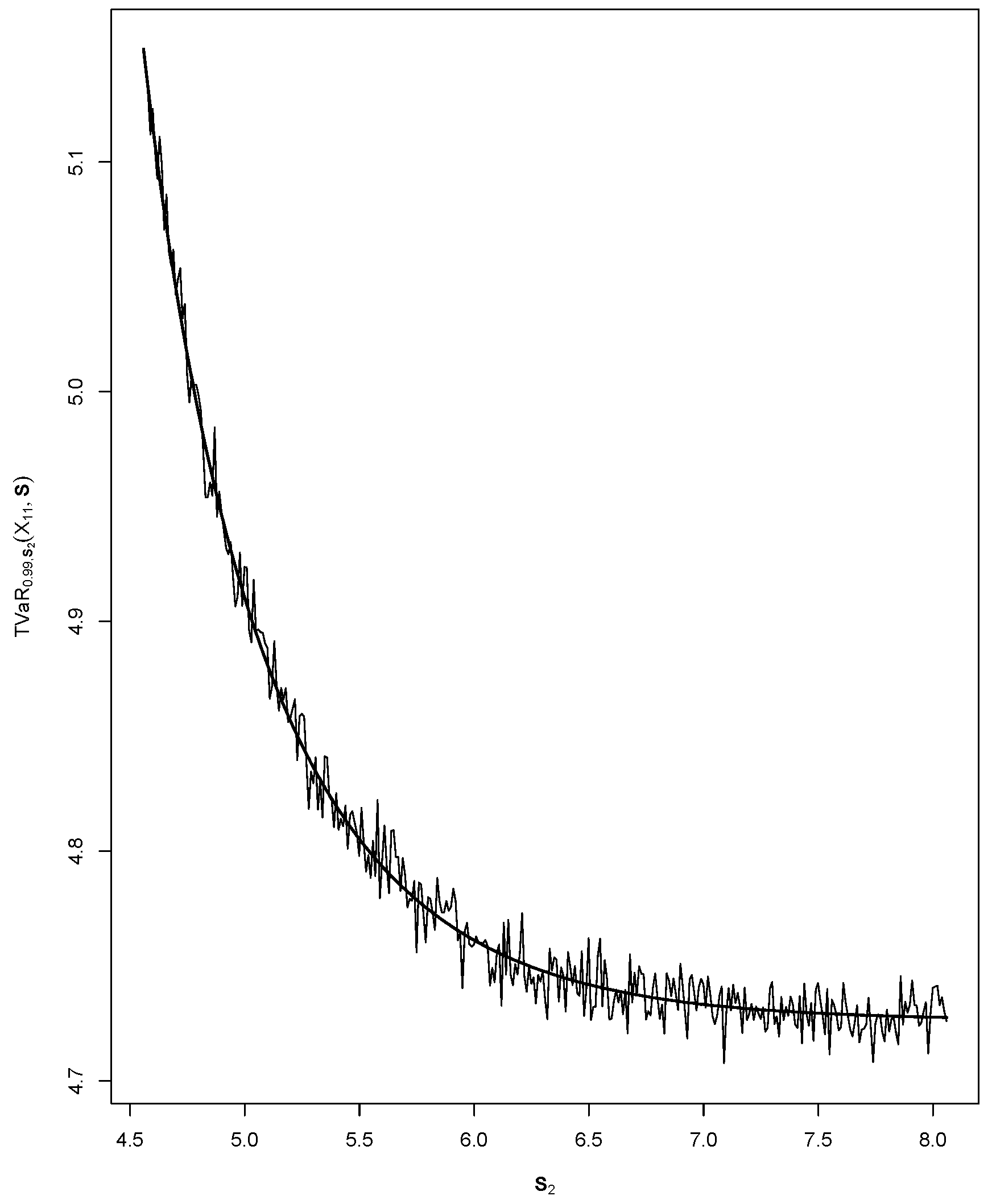
Figure 1 shows the effectiveness of our approximation using importance sampling. Note that calculations were instantaneous with $N=$ 1,000,000 and that ${\displaystyle \sum _{s_2\ge {\mathrm{VaR}}_{0.99}\left(S_2\right)}{\left({\underline{\mathrm{TVaR}}}_{\alpha ,s_2}(X_{11};\mathbf{S})-{\underline{\ddot{\mathrm{TVaR}}}}_{\alpha ,s_2}(X_{11};\mathbf{S})\right)}^2=0.0366}$.

4. Criteria for Capital Allocation Finite Sets

In this section, we present three different methods to derive the contributions of the portfolio’s risks. Each one results in solving an optimization function. Since multivariate TVaR’s are level sets, the resulting contributions are also sets. They provide an amount of capital for a level α and for each value of $x_k$. As stated in the Introduction, regulators aim to establish fixed amounts for the overall business, and the importance of the risk contributions has become essential over time, although it has always been an enterprise risk management matter. Our objective here is to evaluate the contribution of each risk $X_{ij}$ in $S_j=X_{1j}+\cdots +X_{nj}$ given ${\mathbf{S}}_{\backslash j}=(S_1,\cdots ,S_{j-1},S_{j+1},\cdots ,S_k)$, $i=1,\cdots ,n$, $j=1,\cdots ,k$.

As ${\underline{\mathrm{TVaR}}}_{\alpha ,{\mathbf{s}}_{\backslash j}}(X_{ij};\mathbf{S})$ is a function of ${\mathbf{s}}_{\backslash j}=(s_1,\cdots ,s_{j-1},s_{j+1},\cdots ,s_k)$, it will be interesting to derive procedures allowing one to find an optimal vector ${\mathbf{s}}_{\backslash j}^{*}=(s_1^{*},\cdots ,s_{j-1}^{*},s_{j+1}^{*},\cdots ,s_k^{*})$ in order to summarize the multivariate lower orthant TVaR-based contribution function ${\mathbf{s}}_{\backslash j}\to {\underline{\mathrm{TVaR}}}_{\alpha ,{\mathbf{s}}_{\backslash j}}(X_{ij};\mathbf{S})$ by a single value ${\underline{\mathrm{TVaR}}}_{\alpha ,{\mathbf{s}}_{\backslash j}^{*}}(X_{ij};\mathbf{S})$. The three methods provide us with a finite size matrix, based on optimization criteria. Hence, the lower orthant TVaR-based contributions are given by:

$$\begin{array}{c}{\underline{\mathrm{TVaR}}}_{\alpha ,\mathbf{s}}\left(\mathbf{S}\right)=\left(\begin{array}{c}{\underline{\mathrm{TVaR}}}_{\alpha ,s_{\backslash 1}^{*}}(X_{11};\mathbf{S}),\cdots ,{\underline{\mathrm{TVaR}}}_{\alpha ,s_{\backslash k}^{*}}(X_{1k};\mathbf{S})\\ \\ ⋮\\ \\ {\underline{\mathrm{TVaR}}}_{\alpha ,s_{\backslash 1}^{*}}(X_{n1};\mathbf{S}),\cdots ,{\underline{\mathrm{TVaR}}}_{\alpha ,s_{\backslash k}^{*}}(X_{nk};\mathbf{S})\end{array}\right).\end{array}$$

For each method presented, one can find analogous results for the multivariate upper orthant TVaR-based contributions.

4.1. Orthogonal Projection Based on the Multivariate Lower Orthant VaR

We start by defining the vectors:

$${\mathcal{V}}_{\alpha ,{\mathbf{s}}_{\backslash j}}=\left(s_1,\cdots ,s_{j-1},{\underline{\mathrm{VaR}}}_{\alpha ,{\mathbf{s}}_{\backslash j}}\left(\mathbf{S}\right),s_{j+1},\cdots ,s_k\right)$$

and:

$${\mathcal{V}}_{\alpha }=\left({\mathrm{VaR}}_{\alpha }\left(S_1\right),\cdots ,{\mathrm{VaR}}_{\alpha }\left(S_k\right)\right).$$

The objective of this approach is to determine for all $j=1,\cdots ,k$ the optimal solution: ${\mathbf{s}}_{\backslash j}^{*}=(s_1^{*},\cdots ,s_{j-1}^{*},s_{j+1}^{*},\cdots ,s_k^{*})$, for

$$\underset{{\mathbf{s}}_{\backslash j}\in {\mathcal{F}}_j}{min}||{\mathcal{V}}_{\alpha ,{\mathbf{s}}_{\backslash j}}-{\mathcal{V}}_{\alpha }||,$$

where $\parallel ·\parallel$ denote the the Euclidean distance and:

$${\mathcal{F}}_j=\left\{(s_1,\cdots ,s_{j-1},s_{j+1},\cdots ,s_k):s_i\ge {\mathrm{VaR}}_{\alpha }\left(S_i\right),i\ne j\right\}.$$

For fixed $j=1,\cdots ,k$, the vector of TVaR-based contributions of $X_{ij}$ in $S_j$, $i=1,\cdots ,n$ is then given by:

$$\left({\underline{\mathrm{TVaR}}}_{{}_{\alpha ,{\mathbf{s}}_{\backslash j}^{*}}}(X_{1j};\mathbf{S}),\cdots ,{\underline{\mathrm{TVaR}}}_{{}_{\alpha ,{\mathbf{s}}_{\backslash j}^{*}}}(X_{nj};\mathbf{S})\right)$$

where ${\underline{\mathrm{TVaR}}}_{\alpha ,{\mathbf{s}}_{\backslash j}^{*}}(X_{ij};\mathbf{S})$ is given by Proposition 4.

4.2. Orthogonal Projection Based on the Multivariate Lower Orthant TVaR

This method considers TVaR risk measures in order to build a criterion to obtain optimal values. First, we define:

$$T{\mathcal{V}}_{\alpha ,{\mathbf{s}}_{\backslash j}}=\left(s_1,\cdots ,s_{j-1},{\underline{\mathrm{TVaR}}}_{\alpha ,{\mathbf{s}}_{\backslash j}}\left(\mathbf{S}\right),s_{j+1},\cdots ,s_k\right)$$

and:

$$T{\mathcal{V}}_{\alpha }=\left({\mathrm{VaR}}_{\alpha }\left(S_1\right),\cdots ,{\mathrm{VaR}}_{\alpha }\left(S_{j-1}\right),{\mathrm{TVaR}}_{\alpha }\left(S_j\right),{\mathrm{VaR}}_{\alpha }\left(S_{j+1}\right),\cdots ,{\mathrm{VaR}}_{\alpha }\left(S_k\right)\right).$$

The objective is to find ${\mathbf{s}}_{\backslash j}^{*}=(s_1^{*},\cdots ,s_{j-1}^{*},s_{j+1}^{*},\cdots ,s_k^{*})$, the solution to the following minimization problem:

$$\underset{{\mathbf{s}}_{\backslash j}\in {\mathcal{F}}_j}{min}||T{\mathcal{V}}_{\alpha ,{\mathbf{s}}_j}-T{\mathcal{V}}_{\alpha }||.$$

The values of ${\mathbf{s}}_{\backslash j}^{*}$ resulting from this optimization problem are then used to compute, for fixed $j=1,\cdots ,k$, the vector of TVaR-based contributions of $X_{ij}$ in $S_j$, $i=1,\cdots ,n$ given by:

$$\left({\underline{\mathrm{TVaR}}}_{{}_{\alpha ,{\mathbf{s}}_{\backslash j}^{*}}}(X_{1j};\mathbf{S}),\cdots ,{\underline{\mathrm{TVaR}}}_{{}_{\alpha ,{\mathbf{s}}_{\backslash j}^{*}}}(X_{nj};\mathbf{S})\right).$$

4.3. Orthogonal Projection of Multivariate Lower and Upper Orthant TVaR-Based Contributions

The last criterion is based on the lower orthant TVaR-based contributions. For that method, we define the vectors:

$$T{\mathcal{VC}}_{\alpha ,{\mathbf{s}}_{\backslash j}}^{\left(i\right)}=\left({\mathrm{VaR}}_{\alpha }\left(S_1\right),\cdots ,{\mathrm{VaR}}_{\alpha }\left(S_{j-1}\right),{\underline{\mathrm{TVaR}}}_{{}_{\alpha ,{\mathbf{s}}_{\backslash j}}}(X_{ij};\mathbf{S}),{\mathrm{VaR}}_{\alpha }\left(S_{j+1}\right),\cdots ,{\mathrm{VaR}}_{\alpha }\left(S_k\right)\right)$$

and:

$$T{\mathcal{VC}}_{\alpha }^{\left(ij\right)}=\left(s_1,\cdots ,s_{j-1},{\underline{\mathrm{TVaR}}}_{{}_{\alpha }}\left(X_{ij}\right),s_{j+1},\cdots ,s_k\right).$$

For fixed $i=1,\cdots ,n$, we find ${\mathbf{s}}_{\backslash j}^{\left(i\right)}=(s_1^{\left(i\right)},\cdots ,s_{j-1}^{\left(i\right)},s_{j+1}^{\left(i\right)},\cdots ,s_k^{\left(i\right)})$ by solving:

$$\underset{{\mathbf{s}}_{\backslash j}\in {\mathcal{F}}_j}{min}||T{\mathcal{VC}}_{\alpha ,{\mathbf{s}}_j}^{\left(i\right)}-T{\mathcal{VC}}_{\alpha }^{\left(ij\right)}||,j=1,\cdots ,k.$$

The value ${\mathbf{s}}_{\backslash j}^{\left(i\right)}$ resulting from this optimization problem is then used to compute, for fixed $j=1,\cdots ,k$, the vector of TVaR-based contributions of $X_{ij}$ in $S_j$, $i=1,\cdots ,n$ given by:

$$\left({\underline{\mathrm{TVaR}}}_{{}_{\alpha ,{\mathbf{s}}_{\backslash j}^{\left(1\right)}}}(X_{1j};\mathbf{S}),\cdots ,{\underline{\mathrm{TVaR}}}_{{}_{\alpha ,{\mathbf{s}}_{\backslash j}^{\left(n\right)}}}(X_{nj};\mathbf{S})\right).$$

5. Illustrations

In this section, we illustrate the orthogonal projections sets, based on the criteria presented in Section 4. To simplify the presentation and avoid cumbersome notation, we restrict the application to the bivariate case. A more general multivariate situation can be obtained in a similar manner. Let us consider an investor having two dependent portfolios $(S_1,S_2)$, each of which representing dependent sums of random variables, such that $S_j=X_{1j}+X_{2j}$, $j=1,2$. In such a case, we have:

$$S_{1\backslash 1}=X_{21},S_{1\backslash 2}=X_{11},S_{2\backslash 1}=X_{22}\mathrm{and}{S}_{2\backslash 2}=X_{12}$$

and:

$${\mathbf{S}}_{\backslash 1}=S_2\mathrm{and}{\mathbf{S}}_{\backslash 2}=S_1$$

The investor might be interested in a hedging strategy based on the multivariate TVaR at level $\alpha =0.99$ (using negative returns), which considers the dependence between the losses within and between the portfolios. Such a strategy is therefore based on the expectation of the union of conditional events. In this case, each individual event consists of the loss taking a value above level α. Therefore, it is desirable for the investor to have vector-valued metrics in order to hedge his or her assets. Assume that the dependence structures of the random vectors $(X_{11},S_{1\backslash 1},S_2)$ and $(X_{21},S_{1\backslash 2},S_2)$ are described by Archimedean copulas with generators ${\varphi }_1$ and ${\varphi }_2$, respectively. Therefore, the copula of $(X_{11},X_{21})$ is also Archimedean with generator ϕ. Furthermore, in this specific situation, ${\varphi }_1={\varphi }_2=\varphi$, because the Archimedean copulas are symmetric. Let $F_{ij}$ and $F_{S_j}$ be the distribution functions of $X_{ij}$ and $S_j$, $i,j=1,2$, respectively. Suppose that $X_{ij}\sim \mathrm{Exp}\left({\lambda }_{ij}\right)$, $i,j=1,2$ and that $X_{21}$ and $X_{22}$ are independent, which implies that $S_2\sim \mathrm{Exp}({\lambda }_{21}+{\lambda }_{22})$. For illustration, suppose that ϕ represents the generator of a Clayton copula, expressed by $\varphi \left(t\right)=\frac{(t^{-{\theta }_j}-1)}{{\theta }_j}.$ In this context, the components of the lower orthant TVaR-based contributions of $X_{11}$ and $X_{21}$ on $S_1$ given $S_2$, are given by:

$$\begin{array}{c}\hfill \left({\underline{\mathrm{TVaR}}}_{{}_{\alpha ,s_2}}(X_{11};\mathbf{S}),{\underline{\mathrm{TVaR}}}_{{}_{\alpha ,s_2}}(X_{21};\mathbf{S})\right)\end{array}$$

(7)

obtained from Proposition 4, that is:

$$\begin{array}{c}\hfill {\underline{\mathrm{TVaR}}}_{{}_{\alpha ,s_2}}(X_{11};\mathbf{S})=\frac{1}{F_{{\mathbf{S}}_{\backslash j}}\left({\mathbf{s}}_{\backslash j}\right)-\alpha }E\left[\frac{U{X}_U{\ddot{F}}_{11}(X_U,U-X_U,s_2)}{\underline{k}\left(U\right)}\right]\end{array}$$

(8)

and:

$$\begin{array}{c}\hfill {\underline{\mathrm{TVaR}}}_{{}_{\alpha ,s_2}}(X_{21};\mathbf{S})=\frac{1}{1-\alpha }E\left[\frac{U{X}_U{\ddot{G}}_{21}(X_U,U-X_U,s_2)}{\underline{k}\left(U\right)}\right]\end{array}$$

(9)

where:

$${\ddot{F}}_{11}(x,u-x,s_2)=\frac{{\partial }^2}{\partial x_{11}\partial x_{21}}{F}_{(X_{11},X_{21},S_2)}(x,u-x,s_2)$$

and:

$${\ddot{G}}_{21}(x,u-x,s_2)=\frac{{\partial }^2}{\partial x_{21}\partial x_{11}}{F}_{(X_{21},X_{11},S_2)}(x,u-x,s_2).$$

Since the copulas of $(X_{11},X_{21},S_2)$ and $(X_{21},X_{11},S_2)$ are Archimedean with generator ϕ, then:

$$\begin{array}{ccc}\hfill {\ddot{F}}_{12}(x,u-x,s_2)& =& {\left({\varphi }^{-1}\right)}^{″}\left[\varphi \left(F_{11}\left(x\right)\right)+\varphi \left(F_{21}(u-x)\right)+\varphi \left(F_{S_2}\left(s_2\right)\right)\right]\hfill \\ & & \times {\varphi }^{\prime }\left(F_{11}\left(x\right)\right){\varphi }^{\prime }\left(F_{21}(u-x)\right)F_{11}^{\prime }\left(x\right)F_{21}^{\prime }(u-x)\hfill \end{array}$$

(10)

and:

$$\begin{array}{ccc}\hfill {\ddot{G}}_{12}(x,u-x,s_2)& =& {\left({\varphi }^{-1}\right)}^{″}\left[\varphi \left(F_{21}\left(x\right)\right)+\varphi \left(F_{11}(u-x)\right)+\varphi \left(F_{S_2}\left(s_2\right)\right)\right]\hfill \\ & & \times {\varphi }^{\prime }\left(F_{21}\left(x\right)\right){\varphi }^{\prime }\left(F_{11}(u-x)\right)F_{11}^{\prime }(u-x)F_{21}^{\prime }\left(x\right).\hfill \end{array}$$

(11)

Finally, using the projection methods developed in Section 4, we obtain optimal values $s_2^{*}$, and calculate:

$$\begin{array}{c}\hfill \left({\underline{\mathrm{TVaR}}}_{{}_{\alpha ,s_2^{*}}}(X_{11};\mathbf{S}),{\underline{\mathrm{TVaR}}}_{{}_{\alpha ,s_2^{*}}}(X_{21};\mathbf{S})\right).\end{array}$$

1. Orthogonal projection based on the multivariate lower orthant VaR:

We find the optimal $s_2^{*}$ as the solution of the following minimization:

$$\underset{s_2\ge {\mathrm{VaR}}_{\alpha }\left(S_2\right)}{min}\left\{{\left({\underline{\mathrm{VaR}}}_{{}_{\alpha ,s_2}}\left(\mathbf{S}\right)-{\mathrm{VaR}}_{\alpha }\left(S_1\right)\right)}^2+{\left(s_2-{\mathrm{VaR}}_{\alpha }\left(S_2\right)\right)}^2\right\}.$$

2. Orthogonal projection based on the multivariate lower orthant TVaR:

We compute the optimal $s_2^{*}$, as the solution of the following minimization:

$$\underset{s_2\ge {\mathrm{VaR}}_{\alpha }\left(S_2\right)}{min}\left\{{\left({\underline{\mathrm{TVaR}}}_{{}_{\alpha ,s_2}}\left(\mathbf{S}\right)-{\mathrm{TVaR}}_{\alpha }\left(S_1\right)\right)}^2+{\left(s_2-{\mathrm{VaR}}_{\alpha }\left(S_2\right)\right)}^2\right\}.$$

3. Orthogonal projection of multivariate lower and upper orthant TVaR-based contributions:

For this approach, we look for $s_2^{\left(1\right)}$ and $s_2^{\left(2\right)}$ involved in:

$$\begin{array}{c}\hfill \left({\underline{\mathrm{TVaR}}}_{{}_{\alpha ,s_2^{\left(1\right)}}}(X_{11};\mathbf{S}),{\underline{\mathrm{TVaR}}}_{{}_{\alpha ,s_2^{\left(2\right)}}}(X_{21};\mathbf{S})\right)\end{array}$$

by solving respectively the following optimization functions:

$$\underset{s_2\ge {\mathrm{VaR}}_{\alpha }\left(S_2\right)}{min}\left\{{\left({\underline{\mathrm{TVaR}}}_{{}_{\alpha ,s_2}}(X_{11};\mathbf{S})-{\mathrm{TVaR}}_{{}_{\alpha }}(X_{11};S_1)\right)}^2+{\left(s_2-{\mathrm{VaR}}_{\alpha }\left(S_2\right)\right)}^2\right\}$$

and:

$$\underset{s_2\ge {\mathrm{VaR}}_{\alpha }\left(S_2\right)}{min}\left\{{\left({\underline{\mathrm{TVaR}}}_{{}_{\alpha ,s_2}}(X_{21};\mathbf{S})-{\mathrm{TVaR}}_{{}_{\alpha }}(X_{21};S_1)\right)}^2+{\left(s_2-{\mathrm{VaR}}_{\alpha }\left(S_2\right)\right)}^2\right\}.$$

Table 1. Numerical results of the three orthogonal projection methods with varying dependence levels.

Method	${\underline{\mathbf{TVaR}}}_{{0.99,\mathbf{s}}_2}({\mathbf{X}}_{11};\mathbf{S})$	${\underline{\mathbf{TVaR}}}_{{0.99,\mathbf{s}}_2}({\mathbf{X}}_{21};\mathbf{S})$
$\tau =0.25$
VaR orthogonal projection	24.2932	14.2880
TVaR orthogonal projection	24.9778	14.5104
Contribution orthogonal projection	21.3638	13.6285
$\tau =0.50$
VaR orthogonal projection	24.7322	15.6702
TVaR orthogonal projection	24.7459	15.6752
Contribution orthogonal projection	21.3724	15.0712
$\tau =0.75$
VaR orthogonal projection	25.4680	17.5015
TVaR orthogonal projection	25.4733	15.5036
Contribution orthogonal projection	21.8430	16.0891

presents numerical results with ${\lambda }_{11}=0.2$, ${\lambda }_{21}=0.25$, ${\lambda }_{12}=0.1$, ${\lambda }_{22}=0.5$, $\alpha =0.99$ and a dependence parameter expressed in term of a Kendall’s τ, for ϕ, such that ${\tau }_i=0.25,0.50,0.75$, respectively.

Table 1 illustrates that the orthogonal projection based on the multivariate lower orthant VaR always provides smaller results compared to the orthogonal projection based on the multivariate lower orthant TVaR, which is consistent with previous results in Cossette et al. [13]. Moreover, as the dependence parameter increases, one sees that allocation values also increase, which shows consistency for practical applications.

6. Conclusions

In this paper, we provide a multivariate representation of lower and upper orthant TVaR. We also define the multivariate TVaR-based risk decomposition technique, which is in line with the current regulatory framework and enterprise-wide desire of more conservative risk measures. In addition to providing capital allocation curves that are useful for risk comparison, we suggest different ways to calculate finite sets that allow risk managers to allocate an amount to each risk of the portfolio. We assume that the models are known. However, calculation can be time consuming, and we focus our approximation on importance sampling. Further research could be based on improving those approximation techniques in a multivariate setting.

References

1. M. Sherris. “Solvency, capital allocation, and fair rate of return in insurance.” J. Risk Insur. 73 (2006): 71–96. [Google Scholar] [CrossRef]
2. J.H.T. Kim, and M.R. et Hardy. “A capital allocation based on a solvency exchange option.” Insur. Math. Econ. 44 (2009): 357–366. [Google Scholar] [CrossRef]
3. J. Dhaene, A. Tsanakas, V. Emiliano, and V. et Steven. Optimal Capital Sllocation Principles. MPRA Paper 13574; Munich, Germany: University Library of Munich, 2009. [Google Scholar]
4. J. Dhaene, A. Tsanakas, E.A. Valdez, and S. Vanduffel. “Optimal capital allocation principle.” J. Risk Insur. 79 (2012): 1–28. [Google Scholar] [CrossRef] [Green Version]
5. H. Cossette, M. Mailhot, and E. Marceau. “TVaR-based capital allocation for multivariate compound distributions with positive continuous claim amounts.” Insur. Math. Econ. 50 (2012): 247–256. [Google Scholar] [CrossRef]
6. A. Aziz, and D. Roser. “Capital Allocation and RAPM.” Appl. Stoch. Models Bus. Ind. 27 (2004): 2–16. [Google Scholar]
7. Basel Committee on Banking Supervision. “Trends in Risk Integration and Aggregation.” 2003. Available online: http://www.bis.org (accessed on 24 August 2016).
8. Basel Committee on Banking Supervision. “International Convergence of Capital Measurement and Capital Standards: A Revised Framework.” 2004. Available online: http://www.bis.org (accessed on 24 August 2016).
9. Office of the Superintendent of Financial Institutions. “Own Risk and Solvency Assessment.” 2014. Available online: http://www.osfi-bsif.gc.ca/ (accessed on 24 August 2016).
10. P. Embrechts, and G. Puccetti. “Aggregating operational risk across matrix structured loss data.” J. Oper. Risk 3 (2008): 29–44. [Google Scholar]
11. Office of the Superintendent of Financial Institutions. “Own Risk and Solvency Assessment.” 2014. Available online: http://www.osfi-bsif.gc.ca/ (accessed on 24 August 2016).
12. H. Cossette, M. Mailhot, E. Marceau, and M. Mesfioui. “Bivariate lower and upper orthant Value-at-Risk.” Eur. Actuar. J. 3 (2013): 321–357. [Google Scholar] [CrossRef]
13. H. Cossette, M. Mailhot, E. Marceau, and M. Mesfioui. “Vector-Valued Tail Value-at-Risk and Capital Allocation.” Methodol. Comput. Appl. Prob. 18 (2016): 653–674. [Google Scholar] [CrossRef]
14. C. Acerbi, and D. Tasche. “On the coherence of expected shortfall.” J. Bank. Financ. 26 (2002): 1487–1503. [Google Scholar] [CrossRef]
15. D. Tasche. “Risk Contributions and Performance Measurement.” Available online: http://citeseerx.ist.psu.edu/viewdoc/download?doi=10.1.1.68.9393&rep=rep1&type=pdf (accessed on 23 September 2016).
16. H.H. Panjer. Measurement of Risk, Solvency Requirements and Allocation of Capital within Financial Conglomerates. Research Report; Waterloo, ON, Canada: Institute of Insurance and Pension Research, University of Waterloo, 2002. [Google Scholar]
17. M.J. Goovaerts, E. Van den Borre, and R.J.A. et Laeven. “Managing economic and virtual economic capital within financial conglomerates.” N. Am. Actuar. J. 9 (2005): 77–89. [Google Scholar] [CrossRef]
18. S. Izraylevich, and V. Tsudikman. Automated Option Trading: Create, Optimize, and Test Automated Trading Systems. Upper Saddle River, NJ, USA: Ft Press, 2012. [Google Scholar]
19. M. Denault. “Coherent allocation of risk capital.” J. Risk 4 (2001): 1–34. [Google Scholar] [CrossRef]
20. M. Kalkbrener. “An axiomatic approach to capital allocation.” Math. Financ. 15 (2005): 425–437. [Google Scholar] [CrossRef]
21. A.J. McNeil, R. Frey, and P. Embrechts. Quantitative Risk Management. Princeton, NJ, USA: Princeton University Press, 2005. [Google Scholar]
22. R.S. Targino, G.W. Peters, and P.V. Shevchenko. “Sequential Monte Carlo Samplers for capital allocation under copula-dependent risk models.” Insur. Math. Econ. 61 (2015): 206–226. [Google Scholar] [CrossRef]
23. P. Arbenz, M. Cambou, and M. Hofert. “An Importance Sampling Algorithm for Copula Models in Insurance.” 2014, Submitted manuscript. [Google Scholar]
24. D.L. McLeish. “Bounded relative error importance sampling and rare event simulation.” ASTIN Bull. 40 (2010): 377–398. [Google Scholar] [CrossRef]
25. S.C.K. Lee, and X.S. Lin. “Modeling dependent risks with multivariate Erlang mixtures.” ASTIN Bull. 42 (2012): 153–180. [Google Scholar]
Figure 1. Analytic solution and approximation of TVaR 0 . 99 , s 2 ( X 1 , 1 ; S ) .
Risks 04 00033 g001