Bayesian Option Pricing Framework with Stochastic Volatility for FX Data

Abstract

The application of stochastic volatility (SV) models in the option pricing literature usually assumes that the market has sufficient option data to calibrate the model’s risk-neutral parameters. When option data are insufficient or unavailable, market practitioners must estimate the model from the historical returns of the underlying asset and then transform the resulting model into its risk-neutral equivalent. However, the likelihood function of an SV model can only be expressed in a high-dimensional integration, which makes the estimation a highly challenging task. The Bayesian approach has been the classical way to estimate SV models under the data-generating (physical) probability measure, but the transformation from the estimated physical dynamic into its risk-neutral counterpart has not been addressed. Inspired by the generalized autoregressive conditional heteroskedasticity (GARCH) option pricing approach by Duan in 1995, we propose an SV model that enables us to simultaneously and conveniently perform Bayesian inference and transformation into risk-neutral dynamics. Our model relaxes the normality assumption on innovations of both return and volatility processes, and our empirical study shows that the estimated option prices generate realistic implied volatility smile shapes. In addition, the volatility premium is almost flat across strike prices, so adding a few option data to the historical time series of the underlying asset can greatly improve the estimation of option prices.

1. Introduction

The constant volatility assumption in the original Black–Scholes model has been criticized over the years for its failure to produce the implied volatility smile. Time varying volatility offers a promising remedy to capture the smile. For instance, the autoregressive conditional heteroskedasticity (ARCH) models of [1] and the generalised ARCH (GARCH) models of [2] offer the possibility of capturing many stylized time-varying volatility facts in a time series perspective. However, they were mainly used in the investigation of economic series, until Duan ([3]) proposed a GARCH option pricing framework that enabled the GARCH model estimated from asset return series to be conveniently transformed into a risk-neutral process for option pricing purposes. More precisely, the concept of the locally risk-neutral valuation relationship (LRNVR) was established by [3]. Although this option pricing model successfully captures the volatility skewness of the equity option market, it is inadequate to generate the U-shaped volatility smiles in other option markets, such as commodity and foreign exchange (FX) markets.

Two major drawbacks of the GARCH-type models were pointed out by [4]. First, the constraints imposed on the parameters of these models to ensure a positive conditional variance are often violated during estimation. Second, a random oscillatory behaviour of the conditional variance process is ruled out. For the purpose of option pricing, Hull and White [5] proposed the stochastic volatility (SV) model, which contains an additional unobserved random process in the volatility. Heston [6] extended the SV model to allow for a non-zero correlation between the asset return and its volatility, which is called the leverage effect in financial econometrics. Although SV models are often calibrated to observed option data under the risk-neutral measure, option data are not always available for certain underlying assets. When option data are unavailable, market practitioners must resort to estimating the model under the physical measure using historical asset returns, and then transforming the model into its risk-neutral counterpart for derivative pricing.

Unlike GARCH models, SV models do not admit a computable likelihood function, which makes the estimation a highly challenging task. While the maximum likelihood estimation (MLE) method is infeasible, Cordis and Korby [7] introduced discrete stochastic autoregressive volatility (DSARV) models, in which volatilities only take discrete random values. These models greatly reduce computational costs, because the MLE method can be applied. However, most SV models assume a continuous stochastic volatility, and the Bayesian framework has become a useful alternative for statistical inference. The implementation of Bayesian methods usually requires the construction of a Markov chain Monte Carlo (MCMC) simulation from the intractable joint posterior distribution. Jacquier et al. [8] analysed SV models with a leverage effect by adopting the Gibbs sampling scheme. Shephard and Pitt [9] employed the Metropolis–Hastings scheme for the same problem. Other generalizations include the work of [10,11,12], among others. Choy et al. [13] analysed various FX data using different heavy-tailed SV models and found that there were no leverage effects. Wang et al. [14] considered SV models with leverage (SVL) and a bivariate Student-t error distribution. The t-distribution is expressed in a scale mixture of normal (SMN) representation, which significantly simplifies the Gibbs sampler and dramatically reduces computational time. All of the methods presented above are useful in the estimation of the SV model under the physical measure, but the transformation into the risk-neutral process for option pricing can be a highly non-trivial task.

The risk-neutral valuation for derivative pricing is concerned with the appropriate drift term of the asset return process under the pricing (risk-neutral) measure. However, most SV estimation ignores the drift term, speculating that it can be well estimated by sample mean. An exceptional case is the work by [15], but their drift specification cannot be effectively transformed into a risk-neutral process for option pricing purposes. Bates [16] considered the transformation between the two measures and allowed the parameters of the volatility process to change, but he did not set up the locally risk-neutral valuation formula for option pricing with stochastic volatility.

Inspired by the concept of LRNVR in [3], we propose an SV model that enables a convenient transformation into the risk-neutral process. Our model permits the innovations of the return and volatility processes to have different heavy-tailed SMN distributions. Specifically, we choose a variance gamma (VG) error distribution in the return process and a Student-t error distribution in the volatility process. We shall refer to this SV model as the $VG$-t SV model. For modelling FX data, no leverage effect is assumed. The use of SMN distributions permits an efficient Bayesian inference using MCMC algorithms, and provides a better fit to FX data. The VG distribution ([17]) has thicker tails than the Gaussian distribution, retains finite moments for all orders, and offers a good empirical fit to the data. Assuming a constant volatility, Madan et al. [18] applied the VG process to option pricing and showed that the VG model fitted the volatility smile well. In this paper, we allow the volatility to have a stochastic process. We derive the physical process that can be efficiently transformed into a risk-neutral process for the derivative pricing of FX rates.

This paper also contributes to the literature by the use of the Bayesian framework in option pricing with empirical data. We perform the estimation on an FX rate and then simulate option prices based on the proposed model. We find evidence that heavy-tailed distributions for the FX return and its volatility have important implications. When both the FX return and its volatility marginally follow SMN distributions, the generated implied volatility smile matches the shape of the market observed implied volatility very well. The small gap between the model and market implied volatility smile is almost flat across strike prices. The difference between the model and market implied volatility is often known as the volatility premium, and can be managed if a few option data are available. This is because the volatility premium is quite flat across strike prices.

The remainder of this paper is organized as follows. Section 2 presents the model and problem formulation. Section 3 discusses the Bayesian estimation framework using SMN representations and MCMC methods. The simulations of option prices are also detailed. An empirical study on FX options is shown to justify the potential use of the framework. Specifically, the out-of-sample fit from our framework outperforms the standard Black–Scholes model when compared with market option data. We also discuss how to further improve our framework by considering the volatility premium once some (but not necessarily many) option data are available. Finally, concluding remarks are made in Section 4.

2. Stochastic Volatility Model and Option Pricing

2.1. Problem Formulation

Consider a fixed filtered complete probability space $(\Omega ,\mathcal{F},\mathbb{P},{\mathcal{F}}_{t\ge 0})$, where ${\mathcal{F}}_t$ is the filtration generated by independent processes $\left\{{\epsilon }_t\right\}$ and $\left\{{\eta }_t\right\}$, augmented by the null sets of the data-generating (physical) probability measure $\mathbb{P}$. In addition, ${\mathrm{E}}^{\mathbb{P}}\left[{\epsilon }_t\right]={\mathrm{E}}^{\mathbb{P}}\left[{\eta }_t\right]=0$ for all $t\in \mathbb{N}$. Let $S_t$ be the underlying asset price at time t. We construct the following discrete-time SV model under $\mathbb{P}$:

$$\begin{array}{c}\hfill y_t=f\left({\sigma }_t^2\right)+{\sigma }_t{\epsilon }_t,\end{array}$$

(1)

$$\begin{array}{c}\hfill h_t=\mu +\varphi (h_{t-1}-\mu )+\tau {\eta }_t,\end{array}$$

(2)

where $y_t=ln{S}_t-ln{S}_{t-1}$ is the geometric return of an asset at time t, ${\sigma }_t^2=e^{h_t}$ and $h_t$ are the volatility and log-volatility at time t, and $f\left({\sigma }_t^2\right)$ is the drift of the return process, which is a function of the volatility in general. For the log-volatilities, the conditional mean and conditional variance of $h_t$ are given by

$$\mathrm{E}\left[h_t\right|h_{t-1}]=\mu +\varphi (h_{t-1}-\mu ),and\mathrm{V}\left[h_t\right|h_{t-1}]={\tau }^2,$$

while the unconditional mean and unconditional variance can be derived as

$$\mathrm{E}\left[h_t\right]=\mu ,and\mathrm{V}\left[h_t\right]=\frac{{\tau }^2}{1-{\varphi }^2}.$$

Obviously, μ is the unconditional mean of $h_t$, and τ is the conditional standard deviation of $h_t$. We assume that the persistence ϕ in the volatility equation satisfies $\left|\varphi \right|<1$ to ensure that $h_t$ is stationary.

It remains to specify the drift function $f\left({\sigma }_t^2\right)$ to complete the entire SV model for the asset return process. We choose the drift function that meets the following three requirements.

• It should be a simple model that enables us to apply the standard Bayesian inference via MCMC;
• It should be convenient to transform the model under $\mathbb{P}$ to the model under $\mathbb{Q}$, the risk-neutral probability;
• The resulting $\mathbb{Q}$-process should generate option prices close to market prices.

While the third requirement is justified empirically in a later section, we focus on the former two requirements.

We use SMN distributions to model ${\epsilon }_t$ and ${\eta }_t$ so that the Bayesian inference for SV models reported in the literature can be easily applied. For the second requirement, our model is developed using the concept of LRNVR [3], which requires the following properties.

(P₁)

Equivalent probability measures: $\mathbb{P}\left(A\right)=0$ iff $\mathbb{Q}\left(A\right)=0$ for any event A;

(P₂)

Martingale property: ${\mathrm{E}}^{\mathbb{Q}}\left[\left.S_{t+1}\right|{\mathcal{F}}_t\right]=S_t{e}^r$, where r is the one-step continuously compounded interest rate;

(P₃)

Equivalent local variance: ${\mathrm{V}}^{\mathbb{Q}}\left(\left.y_{t+1}\right|{\mathcal{F}}_t\right)={\mathrm{V}}^{\mathbb{P}}\left(\left.y_{t+1}\right|{\mathcal{F}}_t\right),$

where ${\mathcal{F}}_t$ is the information accumulated up to time t, and $\mathrm{V}(·)$ denotes the variance. Duan [3] offered a sound economic interpretation of these requirements, and showed that they ruled out the local arbitrage opportunities within the GARCH models. In fact, ($P_1$) is a compatibility condition that preserves unlikely events to remain unlikely in both probability measures. ($P_2$) ensures that forward contracts—the simplest derivative contracts—are correctly priced so that no arbitrage opportunity exists in the risk-neutral measure $\mathbb{Q}$, consistent with standard financial econometric theory. ($P_3$) maintains the conditional risk level so that no additional risk is generated or reduced from issuing a derivative.

Inspired by the Girsanov theorem on Itô’s processes, we consider the change of measure by linearly shifting the drift term in the asset return process (1) so that it guarantees ($P_1$) and does not affect the Bayesian inference for SV models. The ($P_2$) of LRNVR implies that the drift term contains the interest rate r under $\mathbb{Q}$. Combining these two considerations, we have

$$\begin{array}{ccc}\hfill y_t& =& r+\beta {\sigma }_t+\mathsf{\Phi }\left({\sigma }_t^2\right)+{\sigma }_t{\epsilon }_t,\hfill \\ \hfill h_t& =& \mu +\varphi (h_{t-1}-\mu )+\tau {\eta }_t,\hfill \end{array}$$

where r is the one-period continuously compounded risk-free interest rate, β is a constant, and $\mathsf{\Phi }\left({\sigma }^2\right)$ is the compensator function enforcing ($P_2$) to hold. In addition, ($P_3$) is satisfied, as the conditional variance is evaluated as ${\sigma }^2$ after the mean shift.

To illustrate our idea, we consider the Gaussian innovations for both return and conditional volatility processes. Set $\mathsf{\Phi }=-{\sigma }_t^2/2$. The unconditional distribution of $h_t$ remains Gaussian. Under $\mathbb{P}$,

$$\begin{array}{c}\begin{array}{c}\hfill y_t=r+\beta {\sigma }_t-\frac{{\sigma }_t^2}{2}+{\sigma }_t{\epsilon }_t,\\ \hfill h_t=\mu +\varphi (h_{t-1}-\mu )+\tau {\eta }_t,\end{array}\end{array}$$

(3)

and a pair of $\mathbb{Q}$-processes $({\epsilon }_t^{\ast },{\eta }_t^{\ast })$ satisfying the LRNVR can then be identified. Specifically, ${\epsilon }_t^{\ast }={\epsilon }_t+\beta$ and ${\eta }_t^{\ast }={\eta }_t$. Clearly, $\mathbb{P}$ and $\mathbb{Q}$ are equivalent. The SV model under $\mathbb{Q}$ is deduced as

$$\begin{array}{c}\hfill y_t^{\ast }=r-\frac{{\sigma }_t^2}{2}+{\sigma }_t{\epsilon }_t^{\ast },\end{array}$$

(4)

$$\begin{array}{c}\hfill h_t^{\ast }={\mu }^{\ast }+\varphi (h_{t-1}^{\ast }-\mu )+\tau {\eta }_t^{\ast }.\end{array}$$

(5)

It is easy to verify that

$$\begin{array}{c}\hfill {\mathrm{E}}^{\mathbb{Q}}\left[S_{t+1}|{\mathcal{F}}_t\right]={\mathrm{E}}^{\mathbb{Q}}\left[\left.S_t{e}^{y_{t+1}}\right|{\mathcal{F}}_t\right]=S_t{e}^r{\mathrm{E}}^{\mathbb{Q}}\left[\left.e^{-\frac{1}{2}{\sigma }_t^2+{\sigma }_t{\epsilon }_t^{\ast }}\right|{\mathcal{F}}_t\right]=S_t{e}^r;\\ \hfill {\mathrm{V}}^{\mathbb{Q}}\left[y_{t+1}|{\mathcal{F}}_t\right]={\sigma }_t^2={\mathrm{V}}^{\mathbb{P}}\left[y_{t+1}|{\mathcal{F}}_t\right].\end{array}$$

The following theorem presents a more general result.

Theorem 1.

Consider the SV model in (1)–(2). Let ${\epsilon }_t^{\ast }={\epsilon }_t+\beta$ and ${\eta }_t^{\ast }={\eta }_t$ for any fixed constant β. If there exists an equivalent measure $\mathbb{Q}$ under which $E^{\mathbb{Q}}\left[{\epsilon }_t^{\ast }\right]=E^{\mathbb{Q}}\left[{\eta }_t^{\ast }\right]=0$ and $M\left(s\right)=E^{\mathbb{Q}}\left[e^{s{\epsilon }_t^{\ast }}\right]<\infty$ for all $s>0,t\in \mathbb{N}$ is the moment generating function (MGF) of ${\epsilon }_t^{\ast }$, then the SV model under $\mathbb{P}$:

$$\begin{array}{c}\begin{array}{c}\hfill y_t=r+\beta {\sigma }_t-lnM\left({\sigma }_t\right)+{\sigma }_t{\epsilon }_t,\\ \hfill h_t=\mu +\varphi (h_{t-1}-\mu )+\tau {\eta }_t,\end{array}\end{array}$$

(6)

admits an SV model under $\mathbb{Q}$ satisfying the LRNVR:

$$\begin{array}{c}\begin{array}{c}\hfill y_t^{\ast }=r-lnM\left({\sigma }_t\right)+{\sigma }_t{\epsilon }_t^{\ast },\\ \hfill h_t^{\ast }=\mu +\varphi (h_{t-1}^{\ast }-\mu )+\tau {\eta }_t^{\ast }.\end{array}\end{array}$$

(7)

Proof of Theorem 1.

As the theorem assumes that there is an equivalent probability measure $\mathbb{Q}$, we only need to prove for the second and third conditions of LRNVR. Using the transformation ${\epsilon }_t^{\ast }={\epsilon }_t+\beta$ and ${\eta }_t^{\ast }={\eta }_t$, the SV model in (6) becomes

$$\begin{array}{c}\hfill y_t=r-lnM\left({\sigma }_t\right)+{\sigma }_t{\epsilon }_t^{\ast },\\ \hfill h_t=\mu -\tau \beta \rho +\varphi (h_{t-1}-\mu )+\tau {\eta }_t^{\ast }.\end{array}$$

As $h_t\in {\mathcal{F}}_{t-1}$, it is easy to check that

$$\begin{array}{c}\begin{array}{c}\hfill {\mathrm{E}}^{\mathbb{Q}}\left[S_{t+1}|{\mathcal{F}}_t\right]={\mathrm{E}}^{\mathbb{Q}}\left[\left.S_t{e}^{y_{t+1}}\right|{\mathcal{F}}_t\right]=S_t{e}^r\frac{{\mathrm{E}}^{\mathbb{Q}}\left[\left.e^{{\sigma }_t{\epsilon }_t^{\ast }}\right|{\mathcal{F}}_t\right]}{M\left({\sigma }_t\right)}=S_t{e}^r;\\ \hfill {\mathrm{V}}^{\mathbb{Q}}\left[y_{t+1}|{\mathcal{F}}_t\right]={\sigma }_t^2={\mathrm{V}}^{\mathbb{P}}\left[y_{t+1}|{\mathcal{F}}_t\right].\end{array}\end{array}$$

(8)

☐

The SV model in (6) has a plausible economic interpretation. A simple consideration may assume a constant drift term m so that

$$y_t=m+{\sigma }_t{\epsilon }_t.$$

When a constant expected geometric return is assumed, it violates the economic belief on the return–risk trade off. In terms of the number of model parameters, both the constant drift SV model and that in (6) contain five basic parameters, and other parameters associated with the distributions of ${\epsilon }_t$ and ${\eta }_t$. Without increasing the number of parameters, the SV model shows that the higher the volatility, the higher the expected geometric return for a positive β. In fact, the β can be viewed as the Sharpe ratio: the excess return over volatility. Thus, our model can be interpreted as a constant Sharpe ratio model in a financial econometrics. Badescu et al. [19] reported that the constant drift model needs a subtle Esscher transform to obtain the $\mathbb{Q}$ process under GARCH models, and the computation of option price could be less straightforward. We find that the constant drift SV model also admits implementation difficulties.

For (6) to be well defined, we must ensure that there is an equivalent probability measure $\mathbb{Q}$ under which the $\mathbb{Q}$ moment-generating function of ${\epsilon }_t^{\ast }$ is well defined. Although it is not necessarily true for arbitrary distributions of ${\epsilon }_t$ and ${\eta }_t$, many implementable SV models which are consistent with Theorem 1 can be developed via SMN distributions.

2.2. The SV Model with VG and t Error Distributions

The examples of SMN distributions include the Student-t, VG distributions, and many others. See [20]. Analyses of models with both Student-t innovations on returns and volatility processes have already been conducted, making it a relatively mature field. However, we do not model ${\epsilon }_t$ using a t distribution, because Theorem 1 requires a finite MGF. To allow heavy-tailed distributions for asset return and its volatility, we consider a standard VG distribution with the shape parameter α for ${\epsilon }_t$, and a standard Student-t distribution with ν degrees of freedom for ${\eta }_t$. Using the MGF of the VG distribution, Theorem 1 brings us the following SV model under $\mathbb{P}$.

$$\begin{array}{cc}\hfill y_t& =r+\beta {\sigma }_t+\alpha ln\left(1-\frac{{\sigma }_t^2}{2\alpha }\right)+{\sigma }_t{\epsilon }_t,\hfill \end{array}$$

(9)

$$\begin{array}{cc}\hfill h_t& =\mu +\varphi (h_{t-1}-\mu )+\tau {\eta }_t,\hfill \end{array}$$

(10)

where

$$M\left({\sigma }_t\right)={\left(1-\frac{{\sigma }_t^2}{2\alpha }\right)}^{-\alpha }.$$

The probability density function (PDF) of the VG distribution and its moments are given in Appendix A.

2.3. Bayesian Framework

Bayesian inference combines expert opinions with observational evidence, supplementing classical statistical inference or the frequentist approach once the likelihood is not trivial to obtain, and is performed via the joint posterior distribution of all model parameters. In this context, unlike the GARCH models, the SV models contain an additional random process in the volatility equation, resulting in an additional latent variable for each observation and an intractable likelihood function which involves very high dimensional integrals. Suppose that N asset returns, $\mathbf{y}\in {\mathbb{R}}^N$, are collected for statistical analysis. Then, there are $N+1$ latent volatility variables, $\mathit{h}=(h_0,h_1,...,h_N)$, in the model. Let $\mathbf{\theta }=(\mu ,\varphi ,{\tau }^2,\alpha ,\nu ,\beta )$ be the vector of parameters of the $VG$-t SV model. The likelihood function is an analytically intractable N-dimensional integral of the form:

$$L\left(\mathbf{\theta }\right)=\int {\Pi }_{t=1}^{N}f\left(y_t|h_1,...,h_N\right)f\left(h_0,...,h_N|\mathbf{\theta }\right)d{h}_0...d{h}_N.$$

The parameters spaces of θ and $\mathit{h}$ together can be viewed as an augmented parameter space. In the Bayesian paradigm, a full Bayesian approach for performing Bayesian inference is via the simulation-based MCMC algorithms, which iteratively sample posterior realisations from the joint posterior distribution

$$f\left(\mathbf{\theta },\mathit{h}|\mathit{y}\right)\propto f\left(\mathit{y}|\mathbf{\theta },\mathit{h}\right)f\left(\mathit{h}|\mathbf{\theta }\right)f\left(\mathbf{\theta }\right),$$

where $f\left(\mathbf{\theta }\right)$ is the PDF of the joint prior distributions of θ.

Since the VG and Student-t distributions belong to the class of SMN distributions, we can facilitate an efficient MCMC algorithm for Bayesian inference using a data augmentation technique. Choy and Chan [20] demonstrated Bayesian inference using univariate SMN distributions, including the VG and Student-t distributions. Therefore, our $VG$-t SV model under the $\mathbb{P}$ measure can be expressed hierarchically as

$$\begin{array}{cc}& y_t|h_t,\mu ,\varphi ,{\tau }^2,{\lambda }_{y_t}\sim N\left(Q,{\lambda }_{y_t}{\sigma }_t\right),\hfill \end{array}$$

(11)

$$\begin{array}{cc}& h_t|h_{t-1},y_t,\mu ,\varphi ,{\tau }^2,{\lambda }_{h_t}\sim N\left(\mu +\varphi (h_{t-1}-\mu ),{\lambda }_{h_t}^{-1}{\tau }^2\right),\hfill \end{array}$$

(12)

$$\begin{array}{cc}& h_0|\mu ,\varphi ,{\tau }^2,{\lambda }_{h_0}\sim N\left(\mu ,\frac{{\tau }^2}{{\lambda }_{h_0}(1-{\varphi }^2)}\right),\hfill \end{array}$$

(13)

$$\begin{array}{cc}& {\lambda }_{y_t}|\alpha \sim Ga\left(\frac{\alpha }{2},\frac{\alpha }{2}\right),t=1,2,...T,\hfill \end{array}$$

(14)

$$\begin{array}{cc}& {\lambda }_{h_t}|\nu \sim Ga\left(\frac{\nu }{2},\frac{\nu }{2}\right),t=0,1,...T,\hfill \end{array}$$

(15)

where $Ga(c,d)$ is the gamma distribution with mean $c/d$. See [20] for Bayesian implementation of SMN distributions and [13] for the SV models. In this setup, ${\lambda }_{h_t}$ and ${\lambda }_{y_t}$ are scale mixture variables which can be used as a global diagnostic of potential outliers ([20]) in the return and volatility equations, respectively. The shape parameters ν and α capture the heavy-tailed features of the innovations in the return and volatility processes. This representation of the $VG$-t SV model enables a simple Gibbs sampler for posterior inference, because the full conditional distributions of the log-volatilities and the scale mixture variables will be the univariate Gaussian and gamma distributions.

To complete the Bayesian framework, we adopt the following prior distributions for model parameters. $\mu \sim N(a_{\mu },b_{\mu }),\beta \sim N(a_{\beta },b_{\beta }),{\tau }^2\sim IG(a_{\tau },b_{\tau }),{\varphi }^{\ast }\sim Be(a_{\varphi },b_{\varphi }),\nu \sim Exp\left(a_{\nu }\right),\alpha \sim Exp\left(a_{\alpha }\right),$ where ${\varphi }^{\ast }=\frac{\varphi +1}{2}$ and $N(·,·),IG(·,·),Be(·,·)$ and $Exp(·)$ are the Gaussian, inverse gamma, beta, and exponential distributions. In the empirical study in Section 3, vague and non-informative prior distributions are assigned to $\mu ,\beta ,{\tau }^2$, and α, respectively. For ${\varphi }^{\ast }$, an informative beta prior distribution is assumed. To ensure the existence of the mean and variance for the Student-t distribution, the exponential prior distribution of the degrees of freedom ν is restricted to the range $(2.01,40)$. To implement the Bayesian $VG$-t SV model, one can easily program the Gibbs sampling scheme to obtain posterior samples of the model parameters and the scale mixtures variables for Bayesian inference. Alternatively, we can use the user-friendly WinBUGS software, which just requires the specification of the model and the prior distributions.

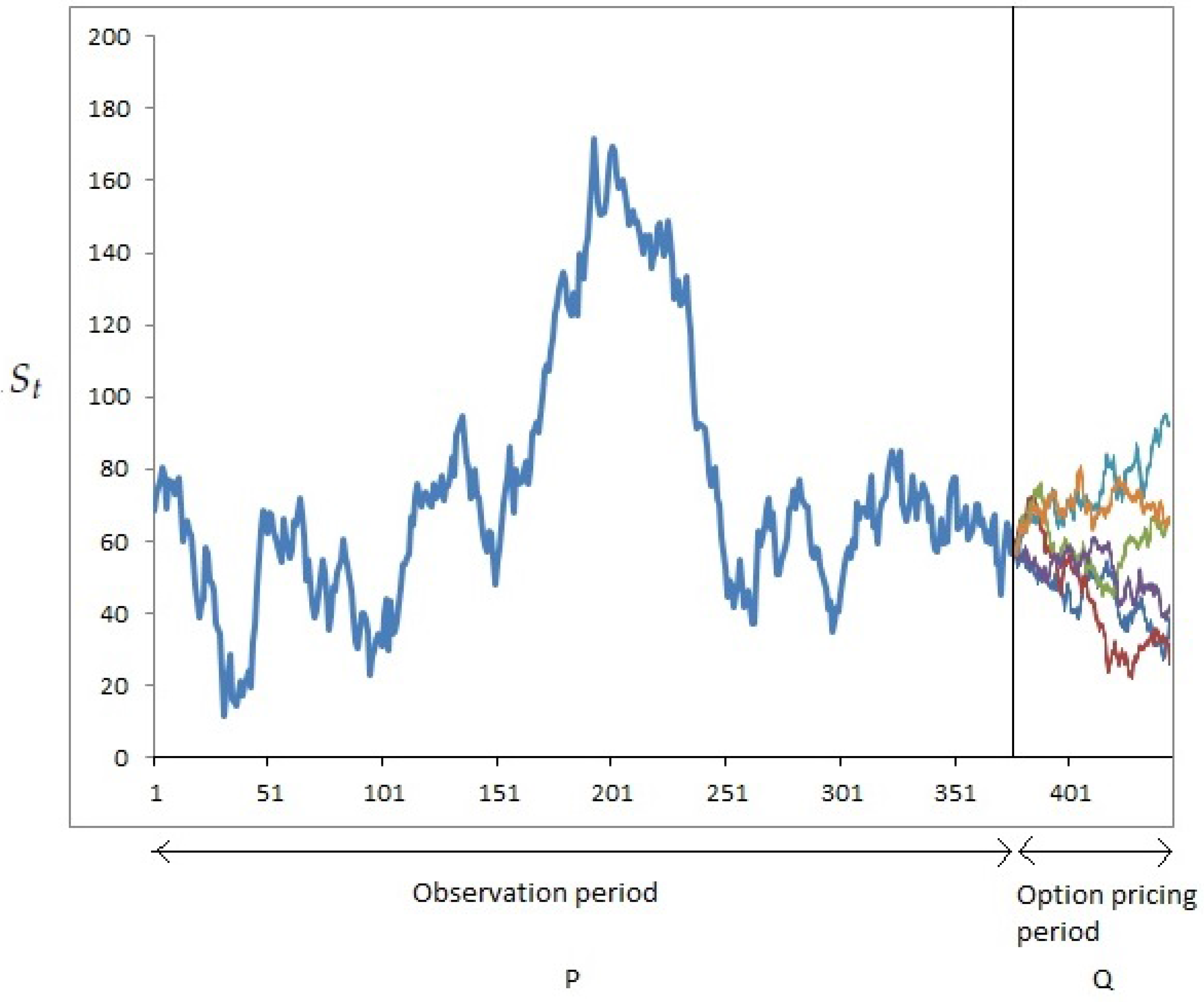
2.4. Option Pricing

Our primary interest is option pricing. We use Figure 1 to explain the valuation procedure. Consider the option with maturity T days after today, when we are standing at time 0 in the perspective of pricing, but time N in the perspective of parameter estimation. Figure 1 shows 375 historical prices of the underlying asset, namely $S_1,...,S_N$, depicted as a random path on the left side. The estimation conducted using the Bayesian approach is carried out based on that path, and the estimated model is defined under $\mathbb{P}$. On the right, five sample paths are generated according to the model under $\mathbb{Q}$ measure for valuing the option numerically. For each generated path, we get $S_T^{\ast }$ at the end. As we consider the European call option in this paper, the payoff would be $\max (S_T^{\ast }-K,0)$, where K is the strike price. With all the simulated sample paths, the option price at time-0 state for pricing (after discounted) can be obtained through the equation

$$C=e^{-rT}{\mathrm{E}}^{\mathbb{Q}}\left\{\max (S_T^{\ast }-K,0)\right\}.$$

(16)

To simulate the $\mathbb{Q}$-process, the posterior mean of each parameter is regarded as the point estimate of the parameter value under $\mathbb{P}$. We transform the model into its risk-neutral equivalent using Theorem 1. The detailed algorithm is summarized in the algorithm below.

Posterior means of the model parameters $\mathbf{\theta }=(\mu ,\varphi ,\beta ,{\tau }^2,\alpha ,\nu )$, and log-volatilities $\mathit{h}=(h_1,...,h_T)$ denoted by $\widehat{\mathbf{\theta }}$ and $\widehat{\mathit{h}}$, are obtained from WinBUGS output, and are used in a process to simulate realisations of the return and log-volatilities under the $\mathbb{Q}$-process. We perform the algorithm as follows.

• Step A: For j = 1:J where J is the number of simulated stock price paths,

  A1:

  Set $h_1^{\ast }=h_N$;

  A2:

  Set $S_0^{\ast }=S_N$;

  A3:

  Sample ${\lambda }_{h_1}^{\ast },...,{\lambda }_{h_T}^{\ast }$ from $Ga\left(\frac{\widehat{\nu }}{2},\frac{\widehat{\nu }}{2}\right)$;

  A4:

  Sample ${\lambda }_{y_1}^{\ast },...,{\lambda }_{y_T}^{\ast }$ from $Ga\left(\frac{\widehat{\alpha }}{2},\frac{\widehat{\alpha }}{2}\right)$;

• Step B: For i = 1:T,

  B1:

  Sample $y_i^{\ast }\left(j\right)$ from $N\left(r+\widehat{\beta }{e}^{h_i^{\ast }\left(j\right)/2},{\lambda }_{y_i\left(j\right)}^{\ast }{e}^{h_i^{\ast }\left(j\right)}\right)$;

  B2:

  Sample $h_i^{\ast }\left(j\right)$ from

  $$N\left(\widehat{\mu }+\widehat{\varphi }\left(h_{i-1}^{\ast }\left(j\right)-\widehat{\mu }\right),{\left({\lambda }_{h_i\left(j\right)}^{\ast }\right)}^{-1}{\widehat{\tau }}^2\right);$$

  B3:

  Set $S_i^{\ast }\left(j\right)=S_{i-1}^{\ast }\left(j\right)e^{y_i^{\ast }\left(j\right)}$;

• Step C: By (16), set

  $$C\cong \frac{e^{-rT}}{J}\sum _{j=1}^{J}max\left(S_T^{\ast }\left(j\right)-K,0\right).$$

  (17)

As each simulated path starts the day that the observations end, $h_{N+1}$—the volatility right after the last point of the observations—is needed as the simulation’s initial volatility. More specifically, Step A shows that the posterior means of $h_{N+1}$ is fixed for all simulated paths. $S_0^{\ast }$ represents the initial price in the simulation part. The rest of the volatilities and mixing parameters are randomly drawn from their posterior distribution, with the hyperparamter values obtained from the estimation. Once $h_{N+1}$ is fixed, the risk-neutral return at $(N+j)$, denoted as $y_j^{\ast }$, is generated, as shown in Step B. Note that $h_1^{\ast }$ is used in the simulation, where $h_1^{\ast }$ and $h_{N+1}$ are related through Theorem 1. Then, option price is obtained through Step C.

3. Empirical Studies

This section examines the empirical performance of the proposed approach in FX option pricing. We collect the daily returns of an FX rate, estimate the $VG$-t SV model parameters with the proposed Bayesian framework, and simulate option prices under the risk-neutral measure. The empirical performance is based on the out-of-sample comparison between the estimated option prices and the market-observed option prices. We pretend that the market option prices are unavailable during our implementation. The option prices evaluated by the Black-Scholes (BS) formula are also reported as a benchmark. Although it is known that GARCH option pricing models perform well in the FX market, they fail to capture the U-shaped volatility smile. By fitting our proposed $VG$-t SV model to the FX market data, we empirically show that our model overcomes this problem by providing a set of implied volatilities within the bid-ask spread of the market-observed implied volatility smile.

Specifically, the estimation is implemented using the WinBUGS package (http://www.mrc-bsu.cam.ac.uk/bugs/) in R. We implement a Gibbs sampler by running a single Markov chain for 20,000 iterations and discarding the first 3000 iterations as the burn-in period to better guarantee the convergence of the estimation result. Sampling procedures and prior distributions are chosen according to Section 2.3. After estimation, simulation for option pricing starts at the last value of observation. From this starting point, we generate $J=8000$ FX rates under the risk-neutral measure according to Section 2.4. Based on the simulated option prices across different strike prices, we calculate the implied volatility and make a comparison with BS formula and the market-observed volatility smile.

3.1. FX Market Data

The empirical study uses one year of data points on the YEN–USD exchange rate from 1 March 2012 to 28 February 2013. To confirm that the $VG$-t SV model is the best model, the FX data is also fitted by the basic SV models ([13]) with N-N (normal-normal), t-t, $VG$-$VG$ and t-$VG$ error distributions in the innovations terms. The Deviance Information Criterion (DIC) and Bayesian Information Criterion (BIC) values of the five models are displayed in

Table 1. Deviance information criterion (DIC) and Bayesian information criterion (BIC) of stochastic volatility (SV) models with different error distributions. N-N: normal-normal; $VG$: variance gamma.

Model	N-N	t-t	t-$VG$	$VG$-t	$VG$-$VG$
DIC	383.3	379.9	378.6	353.3	360.2
BIC	386.6	376.9	379.7	370.9	371.0

. It is obvious that all models with heavy-tailed error distributions are superior to the model with Gaussian errors. Moreover, the models with $VG$ innovation in the return equation outperform the models with Student-t innovation, and in particular, the $VG$-t SV model is chosen to be the best amongst the five models, according to both DIC and BIC values.

European calls on the YEN–USD exchange rate with different strike prices are collected for out-of-sample comparison, with the strike price ranging from 87.94 to 99.79. Half of the options are in-the-money, while the others are out-of-the-money. We use the one-month Libor rates as the constant interest rate for both the estimation and option simulations.

Table 2. Summary statistics of return data on the foreign exchange (FX) rate.

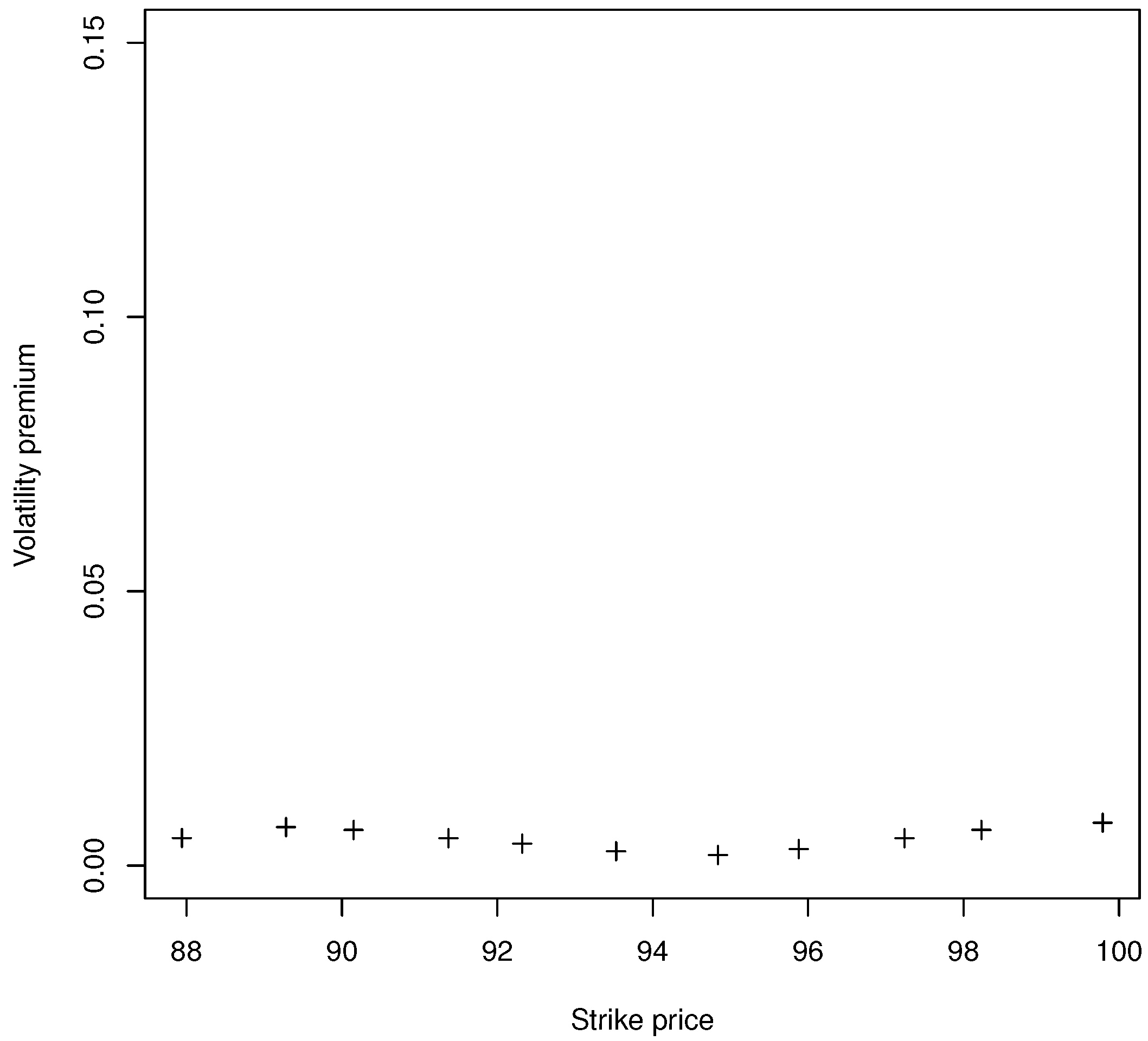
Min.	1st Qu.	Median	Mean	3rd Qu.	Max.	Sd.
$-0.0188$	$-0.0027$	$-0.0003$	0.0002	0.0031	0.0310	0.0052

presents the summary statistics for the source data on the YEN–USD exchange rate. Implied volatilities against different strike prices are given in

Table 3. Implied volatilities of 1-month option data on the FX rate.

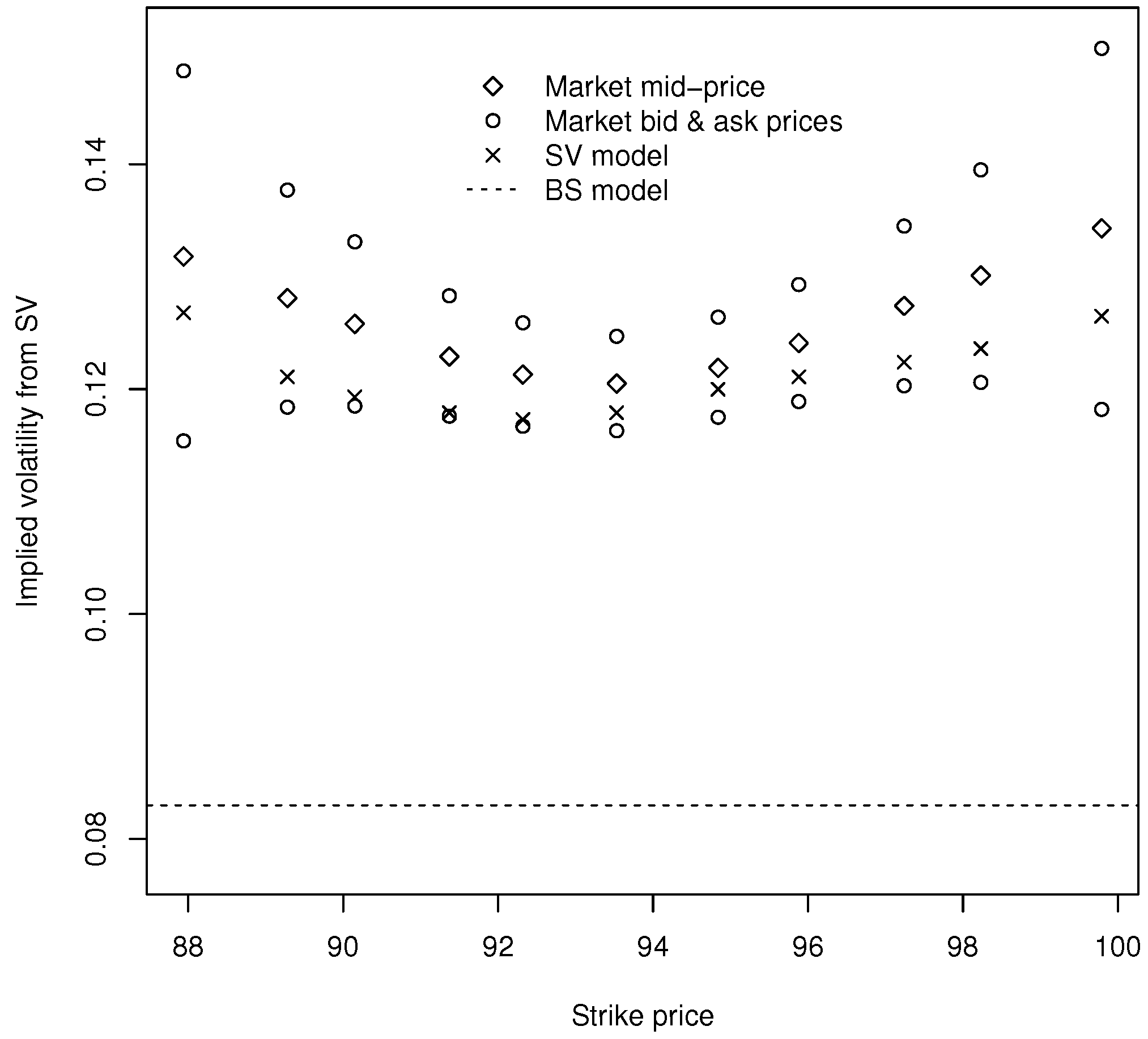
	K = 87.94	K = 89.28	K = 90.15	K = 91.37	K = 92.32	K = 93.53
Mid	0.1318	0.1281	0.1258	0.1229	0.1213	0.1205
Bid	0.1154	0.1184	0.1185	0.1176	0.1167	0.1163
Ask	0.1483	0.1377	0.1331	0.1283	0.1259	0.1247
	K = 93.84	K = 95.88	K = 97.24	K = 98.23	K = 99.79
Mid	0.1219	0.1241	0.1274	0.1301	0.1343
Bid	0.1175	0.1189	0.1203	0.1206	0.1182
Ask	0.1264	0.1293	0.1345	0.1395	0.1503

, in which the market option price is calculated from these market volatilities through the BS formula.

Table 4. Summary statistics of parameters: option on the YEN–USD FX rate from WinBUGS.

Par.	Mean	Sd	95% CI
β	0.078	0.064	($-0.046$ , 0.203)
τ	0.225	0.067	(0.128 , 0.361)
μ	$-10.420$	0.351	($-10.950$, $-9.585$)
ϕ	0.873	0.088	(0.687 , 0.988)
ν	8.176	4.155	(2.531 , 18.114)
α	15.622	8.582	(4.290 , 34.868)

summarizes the estimation results from WinBUGS using the historical FX rates. The small value of ν supports the adoption of a heavy-tailed innovation in the volatility process. The initial spot FX rate for the option simulation was 93.59, on 1 March 2013. The estimated option prices against different strike prices are presented in

Table 5. Results of option prices on the YEN–USD FX rate from the Black-Scholes (BS) model, the SV model, and the market.

Model	K = 87.94	K = 89.28	K = 90.15	K = 91.37	K = 92.32	K = 93.53
Mkt	5.728	4.480	3.711	2.712	2.040	1.335
BS	5.658	4.339	3.507	2.410	1.676	0.934
SV	5.679	4.372	3.555	2.480	1.759	1.020
Model	K = 94.84	K = 95.88	K = 97.24	K = 98.23	K = 99.79
Mkt	0.049	0.509	0.272	0.169	0.077
BS	0.414	0.189	0.054	0.019	0.003
SV	0.497	0.259	0.104	0.055	0.022

. It can also be seen from Figure 2 that our model greatly outperforms the BS model, because the model prices (crosses in the graph) are far over the straight line of the implied volatility from the BS model, and very close to the volatilities implied by market mid-prices. In addition, all implied volatilities from our model are between the market bid and ask volatilities. As actual transactions take place within the bid-ask prices rather than the mid-price, our model offers a reliable tool for practical option prices when the market lacks liquid option data. Furthermore, our $VG$-t SV model captures the volatility smile very well, and this is in consistent with the U-shaped smile of the market-implied volatility. On the contrary, the BS model only offers an unrealistic constant volatility. Although not presented in the figure, the standard GARCH option pricing models also fail to produce such a U-shaped volatility smile for FX options.

Figure 3 plots volatility premium across strike price, which is the difference between the implied volatilities of the market mid-price and the model. The volatility premium is generally flat across strike prices, and the implied volatility from our model can be shifted up to approach the market price if a massive amount of option data is available.

4. Conclusions

In this paper, we propose an SV option pricing model inspired by Duan’s GARCH option pricing model, and extend our model by allowing return and volatility to have VG and Student-t innovations, respectively. The result is an alternative way to price European options when calibration is not applicable. This model enjoys simplicity, reduces simulation inaccuracy, provides an easy and convenient way of transforming the model between physical and risk-neutral measures, and allows the Bayesian inference to apply in the estimation procedure with the benefit of the SMN representation in the MCMC method. In the empirical study, our SV pricing model outperforms its competitive models in the out-of-the-sample test using European call option data, as the model prices are close to the market option prices compared with the BS formula. Furthermore, the model implemented with a Bayesian framework effectively captures the volatility smile in the FX option market, whereas standard GARCH option pricing models only produce a volatility skew.

Future research can focus on alternative specifications of the drift term in the return process, such as the mean reversion process considered by [21]. The proposed Bayesian pricing framework can be generalized to other SV models such as the DSARV model by [7], and to incorporate information for the Volatility Index (VIX) data as suggested by [22].

References

- R.F. Engle. “Autoregressive conditional heteroscedasticity with estimates of variance of United Kingdom inflation.” Econometrica 50 (1982): 987–1008. [Google Scholar] [CrossRef]
- T. Bollerslev. “Generalized autoregressive conditional heteroskedasticity.” J. Econ. 31 (1986): 307–327. [Google Scholar] [CrossRef]
- J.C. Duan. “The GARCH option pricing model.” Math. Financ. 5 (1995): 13–32. [Google Scholar] [CrossRef]
- D.B. Nelson. “Conditional heteroskedasticity in asset returns: A new approach.” Econometrica 59 (1991): 347–370. [Google Scholar] [CrossRef]
- J.C. Hull, and A. White. “The pricing of options on assets with stochastic volatilities.” J. Financ. 42 (1987): 281–300. [Google Scholar] [CrossRef]
- S.L. Heston. “A closed solution for options with stochastic volatility, with application to bond and currency options.” Rev. Financ. Stud. 6 (1993): 327–343. [Google Scholar] [CrossRef]
- A.S. Cordis, and C. Korby. “Discrete stochastic autoregressive volatility.” J. Bank. Financ. 43 (2014): 160–178. [Google Scholar] [CrossRef]
- E. Jacquier, N. Polson, and P. Rossi. “Bayesian analysis of stochastic volatility models (with discussion).” J. Bus. Econ. Stat. 12 (1994): 371–417. [Google Scholar]
- N. Shephard, and M.K. Pitt. “Likelihood analysis of non-Gaussian measurement time series.” Biometrika 84 (1997): 653–667. [Google Scholar] [CrossRef]
- C.A. Abanto-Valle, D. Bandyopadhyay, V.H. Lachos, and I. Enriquez. “Robust Bayesian analysis of heavy-tailed stochastic volatility models using scale mixtures of normal distributions.” Comput. Stat. Data Anal. 54 (2010): 2883–2898. [Google Scholar] [CrossRef] [PubMed]
- R. Meyer, and J. Yu. “BUGS for a Bayesian analysis of stochastic volatility models.” Econ. J. 3 (2000): 198–215. [Google Scholar] [CrossRef]
- J. Yu. “On leverage in a stochastic volatility model.” J. Econ. 127 (2005): 165–178. [Google Scholar] [CrossRef]
- S.T.B. Choy, W.Y. Wan, and C.M. Chan. “Bayesian Student-t stochastic volatility models via scale mixtures.” Adv. Econ. 23 (2008): 595–618. [Google Scholar] [CrossRef]
- J.J.J. Wang, S.K.J. Chan, and S.T.B. Choy. “Stochastic volatility models with leverage and heavy-tailed distributions: A Bayesian approach using scale mixtures.” Comput. Stat. Data Anal. 55 (2011): 852–862. [Google Scholar] [CrossRef]
- C.A. Abanto-Valle, H. Migon, and V.H. Lachos. “Bayesian analysis of heavy-tailed stochastic volatility in mean model using scale mixtures of normal distributions.” J. Stat. Plan. Inference 141 (2011): 1875–1887. [Google Scholar] [CrossRef]
- D.S. Bates. “Maximum likelihood estimation of latent affine processes.” Rev. Financ. Stud. 19 (2006): 909–965. [Google Scholar] [CrossRef]
- D.B. Madan, and E. Seneta. “The variance gamma (V.G.) model for share market returns.” J. Bus. 63 (1990): 511–524. [Google Scholar] [CrossRef]
- D.B. Madan, P.P. Carr, and E.C. Chang. “The variance gamma process and option pricing.” Eur. Financ. Rev. 2 (1998): 79–105. [Google Scholar] [CrossRef]
- A. Badescu, R.J. Elliott, and T.K. Siu. “Esscher transforms and consumption-based models.” Insur. Math. Econ. 45 (2009): 337–347. [Google Scholar] [CrossRef]
- S.T.B. Choy, and J.S.K. Chan. “Scale mixtures in statistics modelling.” Aust. N. Z. J. Stat. 50 (2008): 135–146. [Google Scholar] [CrossRef]
- S.F. Chung, and H.Y. Wong. “Analytical pricing of discrete arithmetic Asian options with mean reversion and jumps.” J. Bank. Financ. 44 (2014): 130–140. [Google Scholar] [CrossRef]
- J. Kanniainen, B. Lin, and H. Yang. “Estimating and using GARCH models with VIX data for option valuation.” J. Bank. Financ. 43 (2014): 200–211. [Google Scholar] [CrossRef]