Change Point Estimation in Panel Data without Boundary Issue

Abstract

Panel data of our interest consist of a moderate number of panels, while the panels contain a small number of observations. An estimator of common breaks in panel means without a boundary issue for this kind of scenario is proposed. In particular, the novel estimator is able to detect a common break point even when the change happens immediately after the first time point or just before the last observation period. Another advantage of the elaborated change point estimator is that it results in the last observation in situations with no structural breaks. The consistency of the change point estimator in panel data is established. The results are illustrated through a simulation study. As a by-product of the developed estimation technique, a theoretical utilization for correlation structure estimation, hypothesis testing and bootstrapping in panel data is demonstrated. A practical application to non-life insurance is presented, as well.

1. Introduction and Main Aims

The problem of an unknown common change in means of the panels is studied, where the panel data consist of N panels, and each panel contains T observations over time. Various values of the change are possible for each panel at some unknown common time $\tau =1,\dots ,T$. The panels are considered to be independent, although this restriction can be weakened. On the other hand, within the panels, the observations are generally not assumed to be independent. This is in accordance with typical assumptions that one can make about real data. A common dependence structure is supposed to be present over the panels. Our main goal is to construct an estimator of a possible change point, which is consistent even in the case of no structural break.

1.1. Current State of the Art

Tests for change point detection in panel data have been proposed by [1] for sufficiently large panel sizes T, i.e., the limiting results were derived under the assumption that T increases over all limits. Testing procedures for the change in panel means with T fixed, which can be relatively small or moderate, were considered in [2]. The change point estimation in panel data for fixed, as well as for unbounded T was studied by [3]. However, the panel change point estimator in [3] is derived only for a situation, where one knows for sure that the change in means occurred within the given time period. This restriction can become insurmountable for some further utilization of the change point estimator, as will be demonstrated later in this paper. In [4], a consistent change point estimator was introduced, requiring no definite knowledge about the existence of the change point in the given panel data. In the case of no change being present, the estimator picks the last observation, which means that no structural break is identified. However, this estimator has several disadvantages. It assumes a certain kind of homoscedasticity in the panels. Further, it does not take into account the possibility that the change may occur right after the first time point. It also assumes conditions that may be viewed as too complicated with regard to verification and model checking. The remaining task is, therefore, to develop a change point estimator that is consistent regardless of the change’s presence/absence. Moreover, such an estimator would gain from allowing heteroscedasticity in the panels, having a broader scope of applications. Besides that, the applicability of the estimator is enhanced by simple consistency conditions and no boundary issue. The boundary issue means that the change point can neither be detected nor estimated when being close to the beginning or to the end of the observation regime.

Further on, Kim [5,6] dealt with the change point estimator under cross-sectional dependence in the panels modeled by a common factor and expanded the estimation problem for more complicated types of structural changes. The first and second order asymptotics that can be used to derive consistent confidence intervals for the time of change in panel data were established by [7]. The panel length T was considered as unbounded and depending on the number of panels N. However, there is some literature on the short panel change point framework where also weighting functions, as we employ later on, are suggested, cf. [8].

1.2. Motivation in Non-Life Insurance

Structural changes in panel data, especially common breaks in means, are wide-spread phenomena. Our primary motivation comes from the non-life insurance business, where associations in many countries uniting several insurance companies collect claim amounts paid by every insurance company each year. Such a database of cumulative claim payments can be viewed as panel data, where insurance company $i=1,\dots ,N$ provides the total claim amount $Y_{i,t}$ paid in year $t=1,\dots ,T$ into the common database. The members of the association can consequently profit from the joint database.

For the whole association, it is important to know whether a possible change in the claim amounts occurred during the observed time horizon. Usually, the time period is relatively short, e.g., 10–15 years. To be more specific, a widely-used and very standard actuarial method for predicting future claim amounts, called chain ladder, assumes a kind of stability of the historical claim amounts. The formal necessary and sufficient condition is derived in [9]. This paper shows a way to detect a possible historical instability.

1.3. Structure of the Paper

The remainder of the paper is organized as follows. Section 2 introduces an abrupt change point model together with stochastic assumptions. An estimator for the change point in panel means is proposed in Section 3. Consequently, the consistency of the considered change point estimator is derived, which covers the first main theoretical contribution. Section 4 contains a simulation study that illustrates the finite sample performance of the estimator. It numerically emphasizes the advantages and disadvantages of the proposed approach. The second main theoretical contribution lies in the panel correlation structure estimation and in the bootstrap add-on justification for hypothesis testing, all provided in Section 5. A practical application of the developed approach to an actuarial problem is presented in Section 6. Proofs are given in the Appendix.

2. Abrupt Change in Panel Data

Let us consider the panel change point model

$$Y_{i,t}={\mu }_i+{\delta }_i\mathcal{I}\{t>\tau \}+{\sigma }_i{\epsilon }_{i,t},1\le i\le N,1\le t\le T;$$

(1)

where ${\sigma }_i>0$ are unknown variance-scaling panel-specific parameters and T is fixed, not depending on N. The possible common change point time is denoted by $\tau \in \{1,\dots ,T\}$. A situation where $\tau =T$ corresponds to no change in means of the panels. The means ${\mu }_i$ are panel individual. The amount of the break in the mean, which can also differ for every panel, is denoted by ${\delta }_i$. There is at most one change per panel in Model (1), and the type of change in the panel mean is abrupt.

Furthermore, it is assumed that the sequences of panel disturbances ${\left\{{\epsilon }_{i,t}\right\}}_t$ are independent. At the same time, the errors within each panel form a weakly-stationary sequence with a common correlation structure. This can be formalized in the following assumption.

Assumption 1.

The vectors ${[{\epsilon }_{i,1},\dots ,{\epsilon }_{i,T}]}^{\top }$ existing on a probability space $(\Omega ,\mathcal{F},\mathsf{P})$ are $iid$ for $i=1,\dots ,N$ with $\mathsf{E}{\epsilon }_{i,t}=0$ and $\mathsf{Var}{\epsilon }_{i,t}=1$, having the autocorrelation function

$${\rho }_t=\mathsf{Corr}\left({\epsilon }_{i,s},{\epsilon }_{i,s+t}\right)=\mathsf{Cov}\left({\epsilon }_{i,s},{\epsilon }_{i,s+t}\right),\forall s\in \{1,\dots ,T-t\},$$

which is independent of the lag s, the cumulative autocorrelation function

$$r\left(t\right)=\mathsf{Var}\sum _{s=1}^t{\epsilon }_{i,s}=\sum _{\left|s\right|<t}(t-|s\left|\right){\rho }_s,$$

and the shifted cumulative correlation function

$$R(t,v)=\mathsf{Cov}\left(\sum _{s=1}^t{\epsilon }_{i,s},\sum _{u=t+1}^v{\epsilon }_{i,u}\right)=\sum _{s=1}^t\sum _{u=t+1}^v{\rho }_{u-s},t<v$$

for all $i=1,\dots ,N$ and $t,v=1,\dots ,T$. The covariance matrix $\mathbf{\Lambda }:=\mathsf{Var}{\left[{\sum }_{s=1}^1{\epsilon }_{1,s},\dots ,{\sum }_{s=1}^T{\epsilon }_{1,s}\right]}^{\top }$ is non-singular.

The sequence ${\left\{{\epsilon }_{i,t}\right\}}_{t=1}^T$ can be viewed as a part of a weakly-stationary process. Note that the within-panel dependent errors do not necessarily need to be linear processes. GARCH processes are a plausible alternative, for instance.

The assumption of independent panels can be relaxed. It would, however, make the setup much more complex, cf. [5]. Consequently, probabilistic tools for dependent data need to be used (e.g., suitable versions of the central limit theorem). Nevertheless, assuming that the claim amounts for different insurance companies are independent is reasonable with regard to real-life experience.

Assumption 2.

There exist constants $\underline{\sigma },\overline{\sigma }>0$ not depending on N, such that

$$\underline{\sigma }\le {\sigma }_i\le \overline{\sigma },1\le i\le N.$$

The assumption of the bounded panel variances from both below and above allows for heteroscedasticity between the panels. In the case when the equiboundedness cannot be satisfied, the panel model can be generalized by introducing weights $w_{i,t}$, which are supposed to be known. Subsequently, claim ratios $Y_{i,t}/w_{i,t}$ can be modeled. Being particular in actuarial practice, it would mean normalizing the total claim amount by the premium received (considered as the weight), since bigger insurance companies are expected to have higher variability in total claim amounts paid.

3. Change Point Estimator

A consistent estimator of the change point in panel data is proposed in [3], but under circumstances that the change occurred for sure. In our situation, we do not know whether a change has occurred or not. Therefore, we modify the estimate proposed by [3] in the following way. If the panel means change somewhere inside $\{1,\dots ,T-1\}$, let the estimate select this break point. If there is no change in panel means, the estimator points out the very last time point T with the probability going to one. In other words, the value of the change point estimate can be T, meaning no change. This is in contrast to [3], where T is not reachable.

Our estimator of the time of change τ in panel data is defined as

$${\widehat{\tau }}_N:=arg\underset{t=1,\dots ,T}{min}\sum _{i=1}^N\left\{\frac{1}{w\left(t\right)}\sum _{s=1}^t{(Y_{i,s}-Y_{i,t})}^2+\frac{1}{w(T-t)}\sum _{s=t+1}^T{(Y_{i,s}-{\tilde{Y}}_{i,t})}^2\right\},$$

(2)

where $Y_{i,t}$ is the average of the first t observations in panel i and ${\tilde{Y}}_{i,t}$ is the average of the last $T-t$ observations in panel i, i.e.,

$$Y_{i,t}=\frac{1}{t}\sum _{s=1}^t{Y}_{i,s}\mathrm{and}{\tilde{Y}}_{i,t}=\frac{1}{T-t}\sum _{s=t+1}^T{Y}_{i,s}.$$

By convention, the value of an empty sum is zero. A sequence of positive weights ${\left\{w\left(t\right)\right\}}_{t=0}^T$ is specified later on.

3.1. Consistency

We postulate additional assumptions on the panel change point model (1) in order to derive the estimator’s consistency. The following conditions take into account that the length T of the observation regime is fixed; that the length T does not depend on the number of panels N; and that the length T can even be relatively small.

Assumption 3.

Let $g\left(t\right):=\frac{t}{w\left(t\right)}\left(1-\frac{r\left(t\right)}{t^2}\right)$ for $t\in \{1,\dots ,T\}$, $g\left(0\right)\equiv 0$, and

$$\begin{array}{cc}\hfill \underset{N\to \infty }{lim}\frac{1}{\sqrt{N}}\left\{\frac{\tau }{\tau +1}\sum _{i=1}^N{\delta }_i^2-\left(g\left(\tau \right)+g(T-\tau )\right)\underset{t=1,\dots ,T}{max}w\left(t\right)\sum _{i=1}^N{\sigma }_i^2\right\}& =\infty ,\hfill \\ \hfill \underset{N\to \infty }{lim}\frac{1}{\sqrt{N}}\left\{\frac{T-\tau }{T-\tau +1}\sum _{i=1}^N{\delta }_i^2-\left(g\left(\tau \right)+g(T-\tau )\right)\underset{t=1,\dots ,T}{max}w\left(t\right)\sum _{i=1}^N{\sigma }_i^2\right\}& =\infty .\hfill \end{array}$$

Assumption 4.

${lim}_{N\to \infty }\frac{1}{N^2}{\sum }_{i=1}^N{\delta }_i^2=0$.

Assumption 5.

$\mathsf{E}{\epsilon }_{1,t}^4<\infty ,t\in \{1,\dots ,T\}$.

Theorem 1 (Change point estimator consistency).

Under Assumptions 1–5,

$$\underset{N\to \infty }{lim}\mathsf{P}[{\widehat{\tau }}_N=\tau ]=1.$$

The formally-postulated estimator’s consistency in Theorem 1 can be practically interpreted: as one observes more and more panels, the probability that the proposed estimator is different from the true unknown change point gets smaller and smaller.

Assumption 3 is not restrictive at all, although it may be seen as a complicated one. For example in the case of independent observations within the panel (i.e., $r\left(t\right)=t$) and the weight function $w\left(t\right)=t^q,$ $q\ge 2$ for $t\in \{1,\dots ,T\}$, $w\left(0\right)=1$, the sequence ${\left\{g\left(t\right)\right\}}_{t=2}^T$ becomes ${\{t^{1-q}-t^{-q}\}}_{t=2}^T$ and is non-increasing. Then, Assumption 3 is automatically fulfilled, if $q=2$ and $\frac{1}{\sqrt{N}}{\sum }_{i=1}^N\left({\delta }_i^2-T^2{\sigma }_i^2\right)\to \infty$ as $N\to \infty$. This also gives us an idea how to choose the weights $w\left(t\right)$. Condition Assumptions 1 and 3, which we impose on the model errors, only pertain to the correlation structure. Hence, our results hold for nearly all stationary time series models of interest, including nonlinear time series, like the ARCH and GARCH processes. Moreover, Assumption 3 controls the trade-off between the size of breaks and the variability of errors. It may be considered as a detectability assumption, because it specifies the value of the signal-to-noise ratio for finding the consistent estimator.

Assumptions 3 and 4 are satisfied, for instance, if $0<\delta \le {\delta }_i\le \Delta$ for all i’s (a common lower and upper threshold for the means’ shifts), ${\delta }^2=\mathcal{O}\left(N^{\zeta }\right)$, $\zeta >0$ and ${\Delta }^2/N\to 0$ as $N\to \infty$ (bearing in mind Assumption 2). Another suitable example of ${\delta }_i$’s for the conditions in Assumptions 3 and 4 can be ${\delta }_i=K{i}^{\eta }$ for some $K>0$ and $0<\eta <1/2$. Condition Assumptions 3 and 4 do not require each panel to have a break. Sometimes, a more restrictive assumption can be assumed instead of Assumptions 3 and 4, e.g.,

$$\underset{N\to \infty }{lim}\frac{1}{N}\sum _{i=1}^N{\delta }_i^2=\infty .$$

(3)

On the one hand, this assumption might be considered as too strong, because a common fixed (not depending on N) value of $\delta ={\delta }_i$ for all i’s does not fulfill (3). On the other hand, (3) is satisfied when ${\delta }_j^2/N\to \infty$ as $N\to \infty$ for some $j\in \mathbb{N}$ and ${\delta }_i=0$ for all $i\ne j$. This stands for a situation when all of the panels do not change in mean, except one panel having a sufficiently large change in mean with respect to the number of panels. Let us notice that one could replace Assumption 3 with a stronger assumption from (3), but it would mean the detectability relation disappearing between the size of breaks and the variability of errors. One would also lose an idea of how to choose the weights. Furthermore, Assumptions E1 and E2 from [4] are more restrictive than Assumption 3, which makes the presented approach even more general.

Various competing consistent estimators of a possible change point can be suggested, e.g., the maximizer of ${\sum }_{i=1}^N{\left[{\sum }_{s=1}^t(Y_{i,s}-t{Y}_{i,T})\right]}^2$, as in [7]. To show the consistency of this estimator, one needs to postulate different assumptions on the cumulative autocorrelation function, and this may be rather complex.

In our opinion, it is erroneously assumed in [3] that only the second moment of the errors is sufficient to prove the consistency result. In particular, Lemma A.1 from [3] has to require the finite fourth errors’ moments, which coincides with Assumption 5.

4. Simulation Study

A simulation experiment was performed to study the finite sample properties of the change point estimator for a common abrupt change in panel means. In particular, the interest lies in the empirical distributions of the proposed estimator visualized via histograms. Random samples of panel data (2000 each time) are generated from the panel change point model (1). The panel size is set to $T=10$ in order to demonstrate the performance of the estimator in the case of small panel length. The number of panels considered is $N=2,5,10,20,50$.

The correlation structure within each panel is modeled via random vectors generated from iid, AR(1) and GARCH(1,1) sequences. The considered AR(1) process has coefficient $\varphi =0.3$. In the case of the GARCH(1,1) process, we use coefficients ${\alpha }_0=1$, ${\alpha }_1=0.1$ and ${\beta }_1=0.2$, which, according to ([10], Example 1), give a strictly stationary process. In all three sequences, the innovations are obtained as iid random variables from a standard normal $N(0,1)$ or Student $t_5$ distribution multiplied by a suitable constant so that the errors possess unit variance (see Assumption 1). The variance-scaling parameters are kept constant for all panels, i.e., ${\sigma }_i=\sigma$ for all i. The sequence of weights is chosen as ${\{w\left(t\right)=t^2\}}_{t=1}^{10}$ and $w\left(0\right)=1$. Monte Carlo simulation scenarios are produced as all possible combinations of the above-mentioned settings, and a selection of the results is listed below.

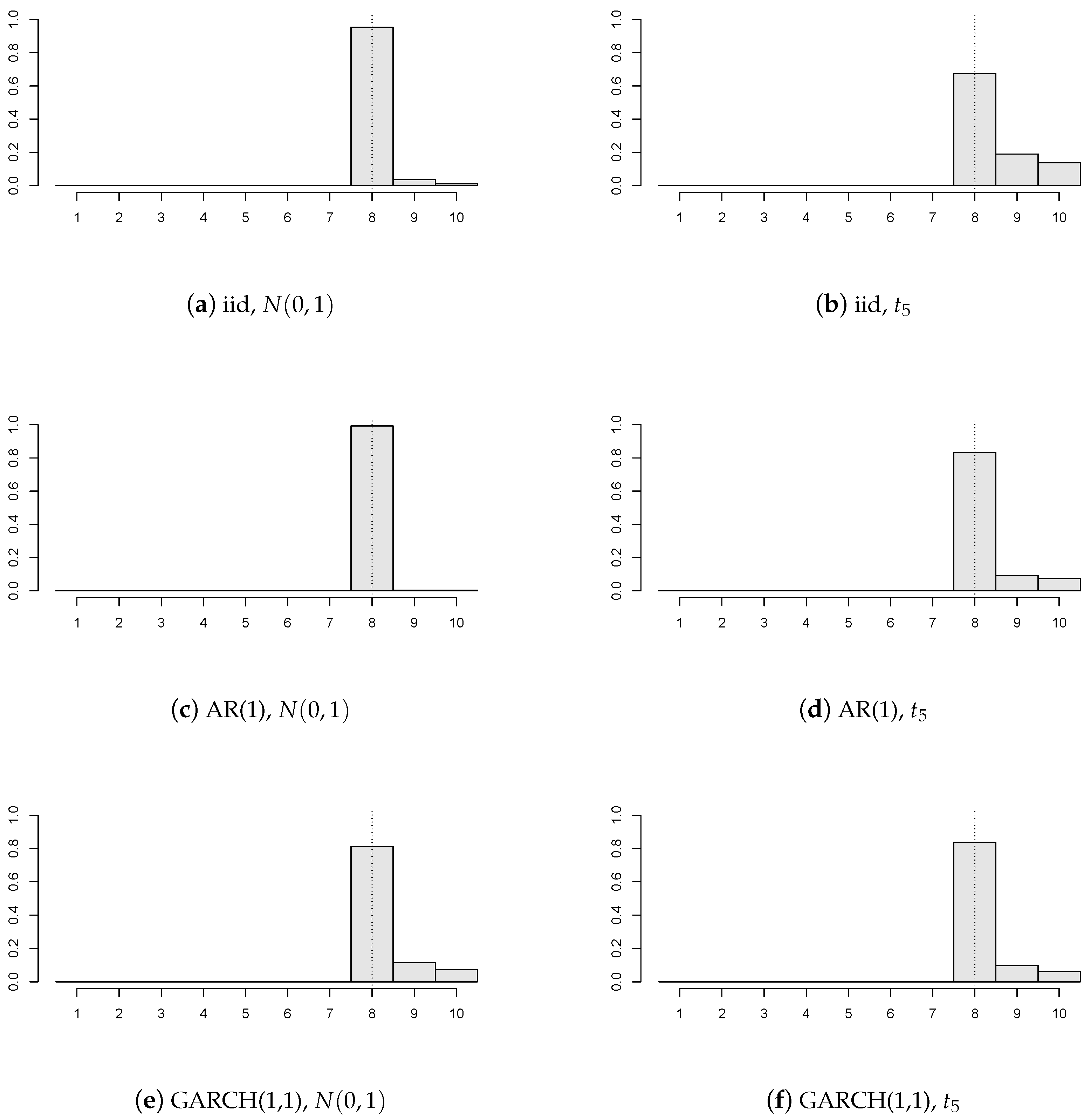
Firstly, we examine the impact of the errors’ distribution and the correlation structure on the change point estimator. Figure 1 contains six different structures of model disturbances, where $\tau =8$ (depicted by the dotted vertical line), $N=20$, $\sigma =0.2$, and all of the panels are subject to the break of value ${\delta }_i\sim U[0,2]$ (i.e., the breaks are independently and uniformly distributed on $[0,2]$).

It can be concluded that the precision of our change point estimator is satisfactory even for a relatively small number of panels regardless of the errors’ structure. Furthermore, innovations with heavier tails yield less precise estimators than innovations with lighter tails (i.e., compare Figure 1a,c,e, versus Figure 1b,d,f). One may notice that the AR(1) errors’ model gives the best estimator’s precision from three correlation structures. This should not be considered as a surprise, because our chosen AR(1) model has a positive autoregression coefficient ($\varphi =0.3$), and therefore, the values of $g\left(\tau \right)$ and $g(T-\tau )$ from Assumption 3 are larger than the values corresponding to the iid errors’ structure. Hence, one can say that the detectability Assumption 3 is satisfied more easily. Loosely speaking, the stronger the positive correlations within the panel, the more “deterministic the behavior” of the random noise and the better the estimator’s precision.

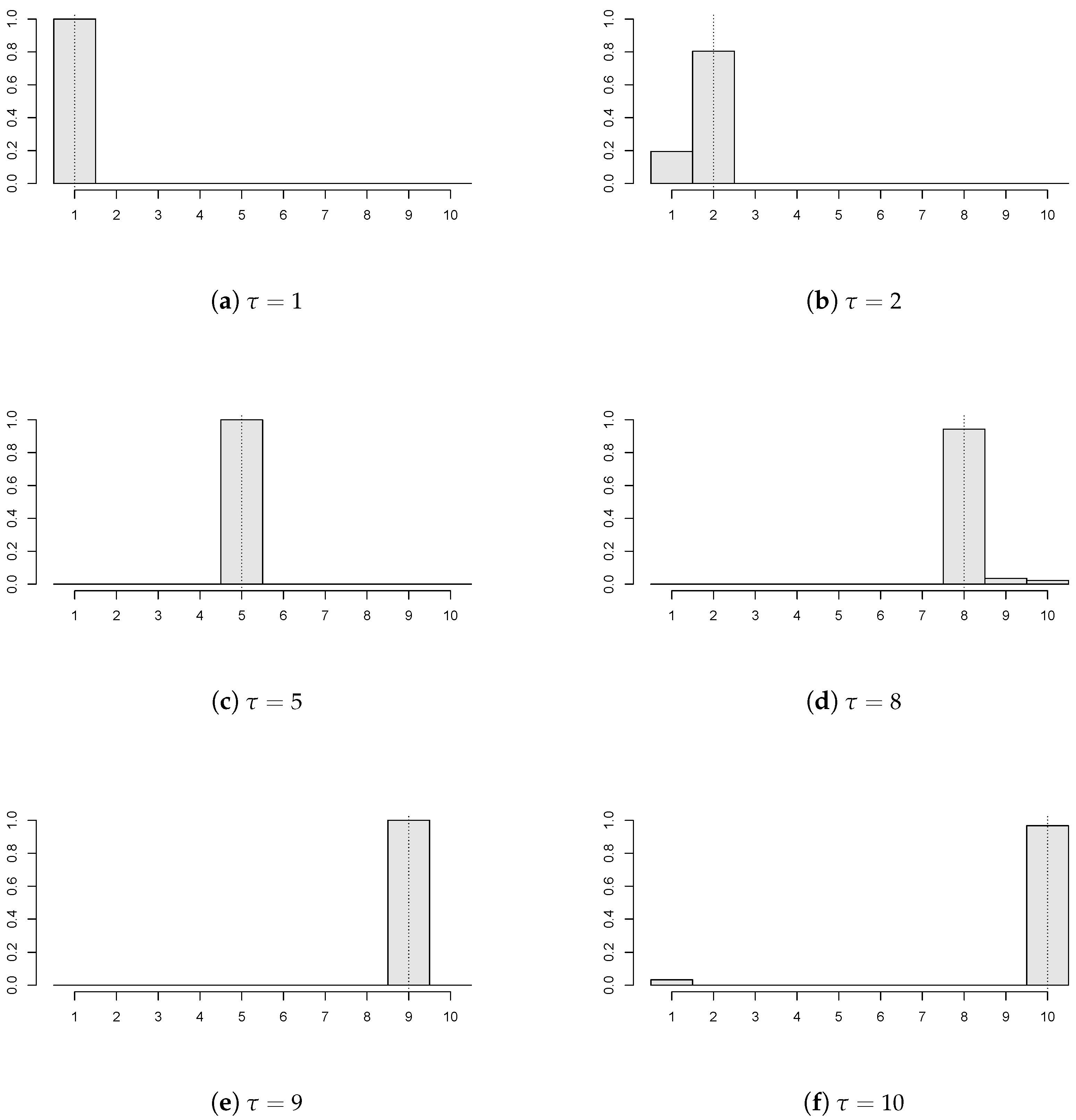
Figure 2 demonstrates that the proposed estimator works reasonably for various locations of the unknown change point. Particularly, six values of the common change point (again, depicted by the dotted vertical line) are chosen ($\tau =1,2,5,8,9,10$) with $N=20$, $\sigma =0.2$; $75\%$ of the panels have a break ${\delta }_i\sim U[0,2]$, and the panel disturbances come from AR(1) with $N(0,1)$ innovations. Recall that $\tau =10$ corresponds to the ‘no change’ situation, and the empirical distribution of the estimator concentrates mainly at the last time point, which is in coherence with the change point formulation from (1).

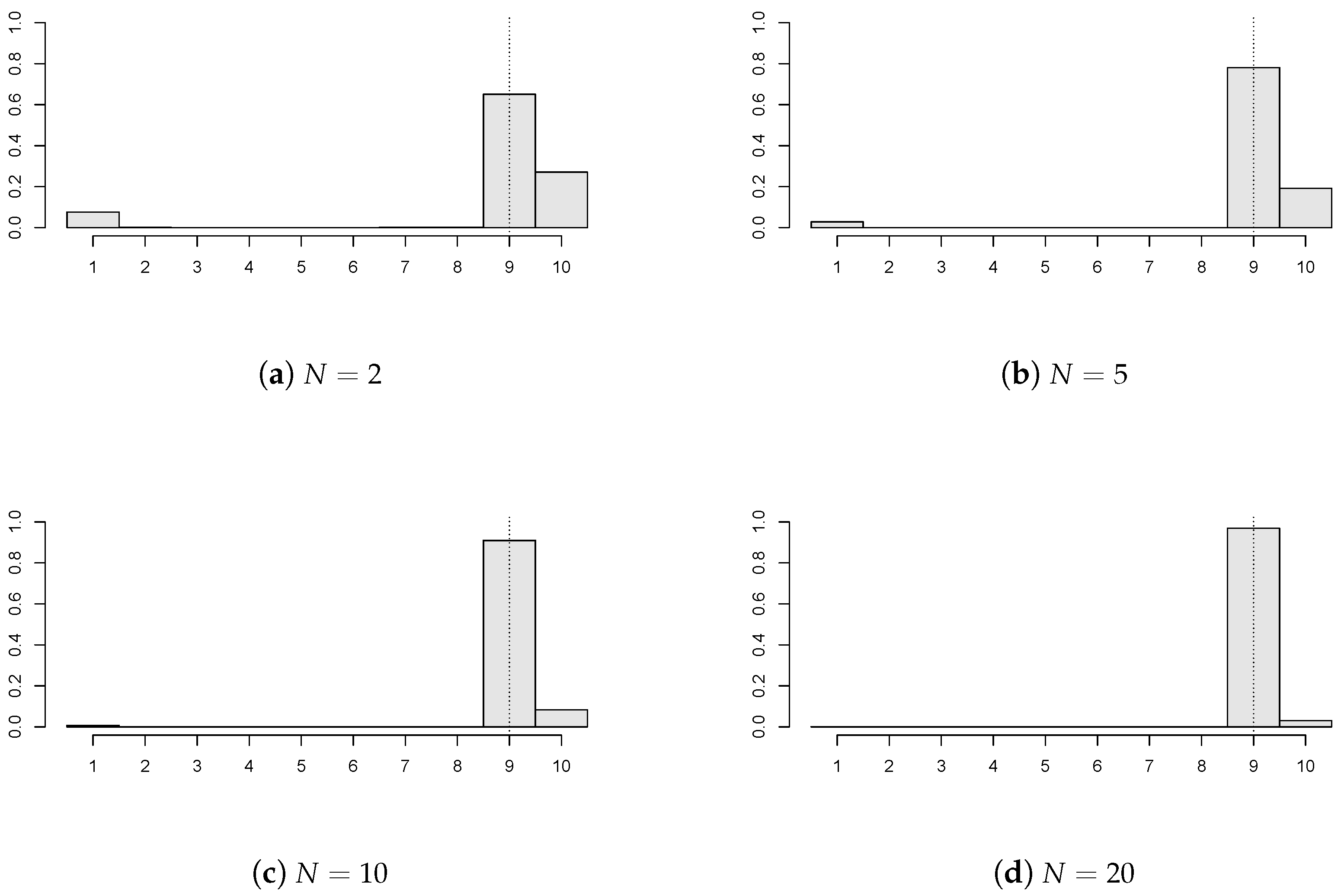
In Figure 3, the impact of the number of panels ($N=2,5,10,20$) is investigated when $\tau =9$, $\sigma =0.2$; $50\%$ of the panels have a break ${\delta }_i\sim U[0,2]$, and the panel disturbances are AR(1) with $t_5$ innovations. It is clear that the precision of ${\widehat{\tau }}_N$ improves markedly as N increases. A higher number of panels, i.e., $N=50$, were also taken into account, and then, $100\%$ precision was achieved. Moreover, longer panels were also simulated (e.g., $T=25$), but these results are not presented here. This is due to the simple reason that the precision of the estimator increases as the panel size gets bigger, which is straightforward and expected.

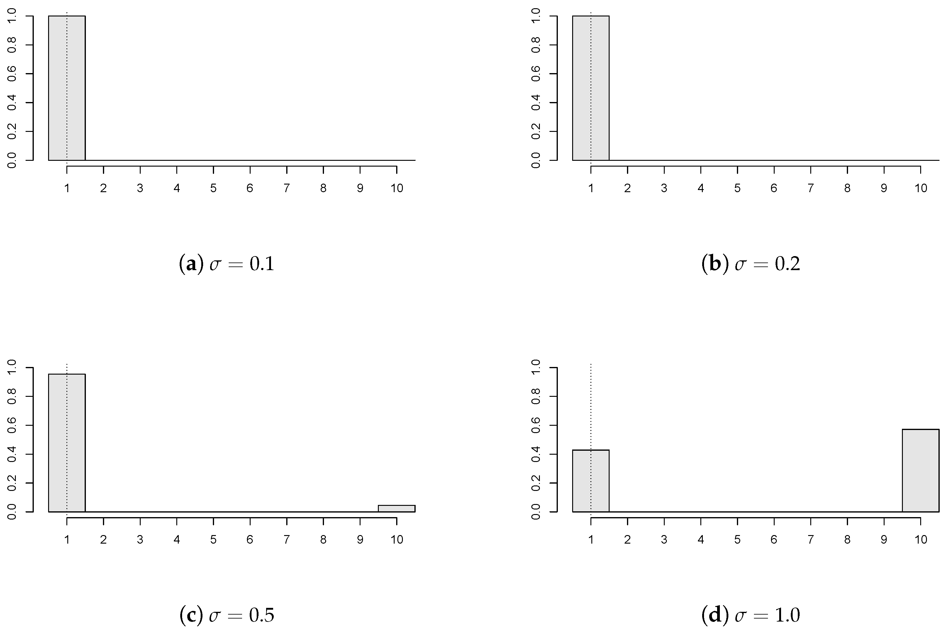
Figure 4 shows the effect of panel variability on the estimator’s performance. In particular, various values of the variance-scaling parameter are considered ($\sigma =0.1,0.2,0.5,1.0$), where $\tau =1$, $N=10$; all of the panels have a break ${\delta }_i\sim U[0,2]$, and the panel disturbances come from GARCH(1,1) with $N(0,1)$ innovations. It can be seen that the less volatile the observations, the more precise the change point estimate. The panel’s variability under the considered dependency can be too high compared to the change size. Then, it would be rather difficult to detect a possible change, as for instance in Figure 4d, which corresponds to $\sigma =1.0$.

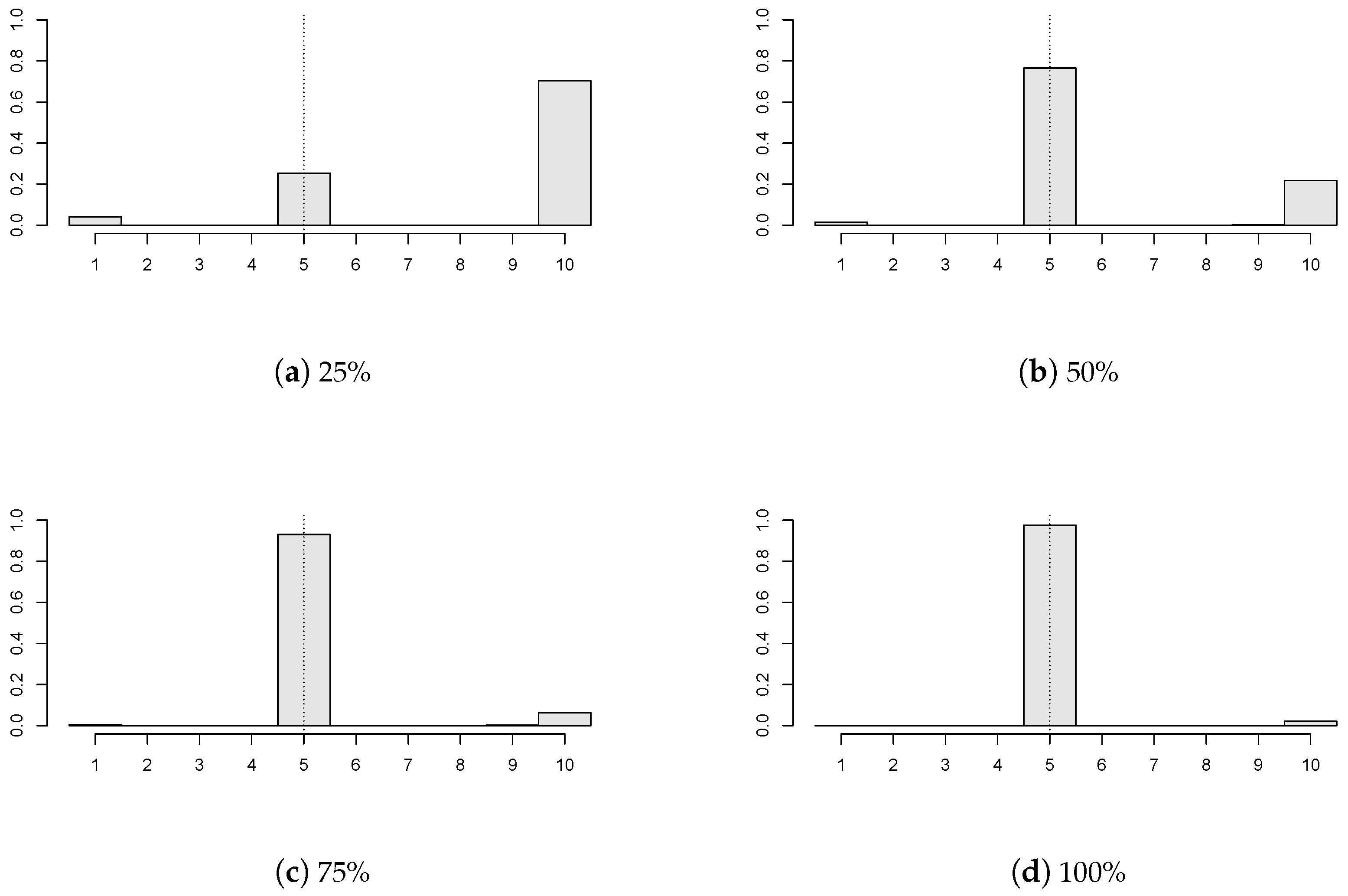
In Figure 5, we examine how different portions of the panels with a change in mean influence the estimator’s precision. Four cases were considered: $25\%$, $50\%$, $75\%$; and all of the panels have a break ${\delta }_i\sim U[0,2]$. Here, $\tau =5$, $N=20$, $\sigma =0.2$; and the panel disturbances are GARCH(1,1) with $t_5$ innovations. One can conclude that higher precision is obtained when a larger portion of panels is subject to change in the mean. If a small number of panels contain a break (for example, Figure 5a), then the change point estimator does not perform well.

5. Theoretical Usage in Hypothesis Testing

Estimation of structural breaks can become an important mid-step in many statistical procedures, e.g., estimation of the panel correlation structure or bootstrapping in hypothesis testing for the change point.

A possible theoretical application of the change point estimation can be motivated as follows. It is required to test the null hypothesis of no change in the means:

$$H_0:\tau =T$$

against the alternative that at least one panel has a change in mean:

$$H_1:\tau <T\mathrm{and}\exists i\in \{1,\dots ,N\}:{\delta }_i\ne 0.$$

Generally, a test statistic ${\mathcal{S}}_{N,T}$ for the change point detection may be constructed as a continuous function of the sums of cumulative residuals, cf. [2]. In particular,

$${\mathcal{S}}_{N,T}\equiv \mathcal{S}\left({\left\{\frac{1}{\sqrt{N}}\sum _{i=1}^N\sum _{r=1}^s(Y_{i,r}-Y_{i,t})\right\}}_{s=1,t=2}^{t-1,T},{\left\{\frac{1}{\sqrt{N}}\sum _{i=1}^N\sum _{r=s+1}^T(Y_{i,r}-{\tilde{Y}}_{i,t})\right\}}_{s=t,t=1}^{T-1,T-1}\right),$$

where $\mathcal{S}(·,·):{\mathbb{R}}^{T\times (T-1)/2}\times {\mathbb{R}}^{T\times (T-1)/2}\to \mathbb{R}$ is continuous. To illustrate, a ratio type test statistic, discussed in [11],

$${\mathcal{S}}_{N,T}=\underset{t=2,\dots ,T-2}{max}\frac{{max}_{s=1,\dots ,t-1}\left|{\sum }_{i=1}^N{\sum }_{r=1}^s(Y_{i,r}-Y_{i,t})\right|}{{max}_{s=t,\dots ,T-1}\left|{\sum }_{i=1}^N{\sum }_{r=s+1}^T(Y_{i,r}-{\tilde{Y}}_{i,t})\right|}$$

is generated by the continuous function

$$\mathcal{S}\left({\left\{a_{s,t}\right\}}_{s=1,t=2}^{t-1,T},{\left\{b_{s,t}\right\}}_{s=t,t=1}^{T-1,T-1}\right)=\underset{t=2,\dots ,T-2}{max}\frac{{max}_{s=1,\dots ,t-1}\left|a_{s,t}\right|}{{max}_{s=t,\dots ,T-1}\left|b_{s,t}\right|}.$$

The test statistic under the null would typically have a known limiting distribution (up to some unknown parameters), which is a function of a Gaussian vector or process. However, its correlation structure is unknown and needs to be estimated. Alternatively, one can avoid the estimation of the correlation structure (which may be considered as a nuisance parameter) by applying a suitable bootstrap procedure. The consistent change point estimator plays also an important role in the validity of the bootstrap algorithm.

5.1. Estimation of Correlation Structure

Since the panels are considered to be independent and the number of panels may be sufficiently large, one can estimate the correlation structure of the errors ${[{\epsilon }_{1,1},\dots ,{\epsilon }_{1,T}]}^{\top }$ empirically. We base the errors’ estimates on residuals

$${\widehat{e}}_{i,t}:=\left\{\begin{array}{cc}{Y}_{i,t}-Y_{i,{\widehat{\tau }}_N},\hfill & t\le {\widehat{\tau }}_N,\hfill \\ Y_{i,t}-{\tilde{Y}}_{i,{\widehat{\tau }}_N},\hfill & t>{\widehat{\tau }}_N.\hfill \end{array}\right.$$

(4)

One may notice that the estimators that cannot result in the last time point are less suitable in the calculation of residuals.

Then, the empirical version of the autocorrelation function is

$${\widehat{\rho }}_t:=\frac{1}{N(T-t)}\sum _{i=1}^N\frac{1}{{\widehat{\sigma }}_i^2}\sum _{s=1}^{T-t}{\widehat{e}}_{i,s}{\widehat{e}}_{i,s+t},$$

where ${\widehat{\sigma }}_i^2:=\frac{1}{T}{\sum }_{s=1}^T{\widehat{e}}_{i,s}^2$ is the estimate of the variance parameter ${\sigma }_i^2$. Consequently, the cumulative autocorrelation function and shifted cumulative correlation function are estimated by

$$\widehat{r}\left(t\right)=\sum _{\left|s\right|<t}(t-|s\left|\right){\widehat{\rho }}_s\mathrm{and}\widehat{R}(t,v)=\sum _{s=1}^t\sum _{u=t+1}^v{\widehat{\rho }}_{u-s},t<v.$$

5.2. Bootstrapping

A wide range of literature has been published on bootstrapping in the change point problem, e.g., [2,12,13]. We build up the bootstrap test on the resampling with the replacement of row vectors ${\left\{[{\widehat{e}}_{i,1},\dots ,{\widehat{e}}_{i,T}]\right\}}_{i=1,\dots ,N}$ corresponding to the individual panels. This provides bootstrapped row vectors ${\left\{[{\widehat{e}}_{i,1}^{*},\dots ,{\widehat{e}}_{i,T}^{*}]\right\}}_{i=1,\dots ,N}$. Then, the bootstrapped residuals ${\widehat{e}}_{i,t}^{*}$ are centered by their conditional expectation $\frac{1}{N}{\sum }_{i=1}^N{\widehat{e}}_{i,t}$, yielding

$${\widehat{Y}}_{i,t}^{*}:={\widehat{e}}_{i,t}^{*}-\frac{1}{N}\sum _{i=1}^N{\widehat{e}}_{i,t}.$$

The bootstrap test statistic is just a modification of the original statistic ${\mathcal{S}}_{N,T}$, where the original observations $Y_{i,t}$ are replaced by their bootstrap counterparts ${\widehat{Y}}_{i,t}^{*}$:

$${\mathcal{S}}_{N,T}^{*}\equiv \mathcal{S}\left({\left\{\frac{1}{\sqrt{N}}\sum _{i=1}^N\sum _{r=1}^s({\widehat{Y}}_{i,r}^{*}-{\widehat{Y}}_{i,t}^{*})\right\}}_{s=1,t=2}^{t-1,T},{\left\{\frac{1}{\sqrt{N}}\sum _{i=1}^N\sum _{r=s+1}^T({\widehat{Y}}_{i,r}^{*}-{\tilde{\widehat{Y}}}_{i,t}^{*})\right\}}_{s=t,t=1}^{T-1,T-1}\right),$$

such that

$${\widehat{Y}}_{i,t}^{*}=\frac{1}{t}\sum _{s=1}^t{\widehat{Y}}_{i,s}^{*}\mathrm{and}{\tilde{\widehat{Y}}}_{i,t}^{*}=\frac{1}{T-t}\sum _{s=t+1}^T{\widehat{Y}}_{i,s}^{*}.$$

The idea behind bootstrapping is to mimic the original distribution of the test statistic by the distribution of the bootstrap test statistic, conditionally on the original data denoted by $\mathbb{Y}\equiv {\left\{Y_{i,t}\right\}}_{i,t=1}^{N,T}$. Recall that it is not known whether some common change in panel means occurred or not. In other words, one does not know whether the data come from the null or the alternative hypothesis.

Theorem 2 (Bootstrap justification).

Suppose that Assumptions 1, 2 and 5 hold. Then,

(i) 

under $H_0$,

$${\mathcal{S}}_{N,T}\underset{N\to \infty }{\overset{\mathcal{D}}{\to }}\mathcal{L};$$

(ii) 

under additional Assumptions 3, 4 and under $H_0$, as well as under $H_1$,

$${\mathcal{S}}_{N,T}^{*}|\mathbb{Y}\underset{N\to \infty }{\overset{\mathcal{D}}{\to }}{\mathcal{L}}^{*}inprobability\mathsf{P};$$

(iii) 

under additional Assumptions 3, 4 and under $H_0$, $\mathcal{L}$ and ${\mathcal{L}}^{*}$ coincide.

The validity of the bootstrap test is assured by Theorem 2. Indeed, the conditional asymptotic distribution of the bootstrap test statistic does not converge to infinity (in probability) under the alternative. In other words, the second part of Theorem 2 holds under $H_0$, as well as $H_1$. In contrast to the bootstrap version of the test statistics, the original test statistic typically explodes over all bounds under the alternative. That is why the bootstrap test statistic can be used correctly to reject the null in favor of the alternative, having sufficiently large N. Moreover, Theorem 2 states that the conditional distribution of the bootstrap test statistic and the unconditional distribution of the original test statistic coincide under the null. Additionally, that is the reason why the bootstrap test approximately keeps the same level as the original test based on the asymptotics (i.e., the test based on the asymptotic distribution of ${\mathcal{S}}_{N,T}$).

A practical choice of the test statistic ${\mathcal{S}}_{N,T}$ can be obtained from, e.g., [14]:

$${\mathcal{S}}_{N,T}=\underset{t=2,\dots ,T-2}{max}\frac{{\sum }_{s=1}^{t-1}{\left[{\sum }_{i=1}^N{\sum }_{r=1}^s(Y_{i,r}-Y_{i,t})\right]}^2}{{\sum }_{s=t}^{T-1}{\left[{\sum }_{i=1}^N{\sum }_{r=s+1}^T(Y_{i,r}-{\tilde{Y}}_{i,t})\right]}^2}$$

or

$${\mathcal{S}}_{N,T}=\underset{t=2,\dots ,T-2}{max}\frac{{max}_{s=1,\dots ,t-1}{\sum }_{i=1}^N{\sum }_{r=1}^s(Y_{i,r}-Y_{i,t})-{min}_{s=1,\dots ,t-1}{\sum }_{i=1}^N{\sum }_{r=1}^s(Y_{i,r}-Y_{i,t})}{{max}_{s=t,\dots ,T-1}{\sum }_{i=1}^N{\sum }_{r=s+1}^T(Y_{i,r}-{\tilde{Y}}_{i,t})-{min}_{s=t,\dots ,T-1}{\sum }_{i=1}^N{\sum }_{r=s+1}^T(Y_{i,r}-{\tilde{Y}}_{i,t})}.$$

Theorem 2 assures that the previously-described bootstrap algorithm can be used in hypothesis testing (change point detection) for the above-mentioned test statistics. Now, the simulated (empirical) distribution of the bootstrap test statistic can be used to calculate the bootstrap critical value, which will be compared to the value of the original test statistic in order to reject the null or not.

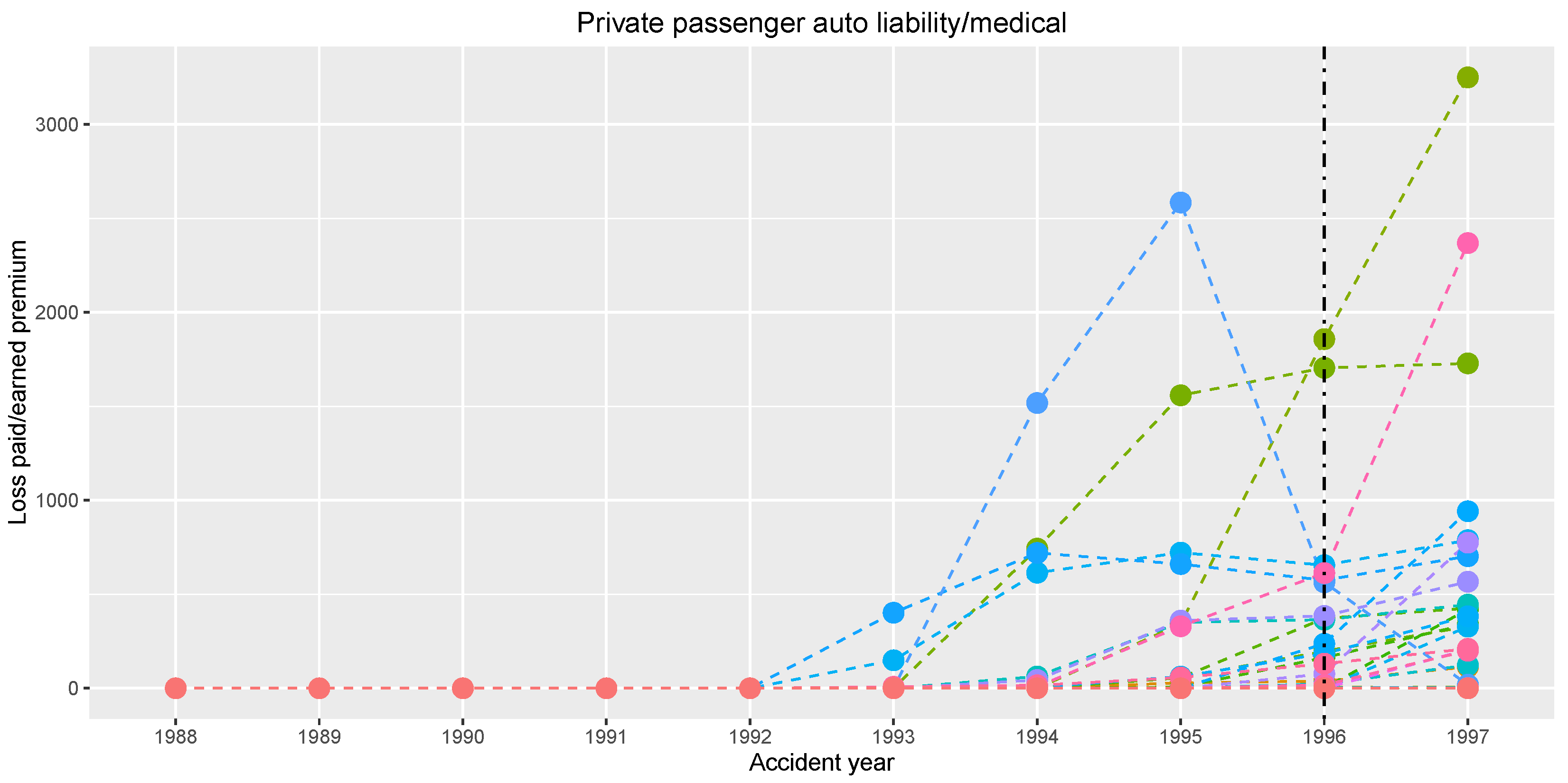
6. Practical Application in Non-Life Insurance

As mentioned in the Introduction, our primary motivation for the change point estimation in panel data comes from the non-life insurance business. The dataset is provided by the National Association of Insurance Commissioners (NAIC) database; see [15]. We concentrate on the ‘private passenger auto liability/medical’ insurance line of business. The data collect records from $N=146$ insurance companies. Each insurance company provides $T=10$ yearly total claim amounts starting from year 1988 up to year 1997. One can consider normalizing the claim amounts by the premium received by company i in year t. That is thinking of panel data $Y_{i,t}/p_{i,t}$, where $p_{i,t}$ is the mentioned premium. This may yield a stabilization of series’ variability, which corresponds to Assumption 2 of bounded variances. 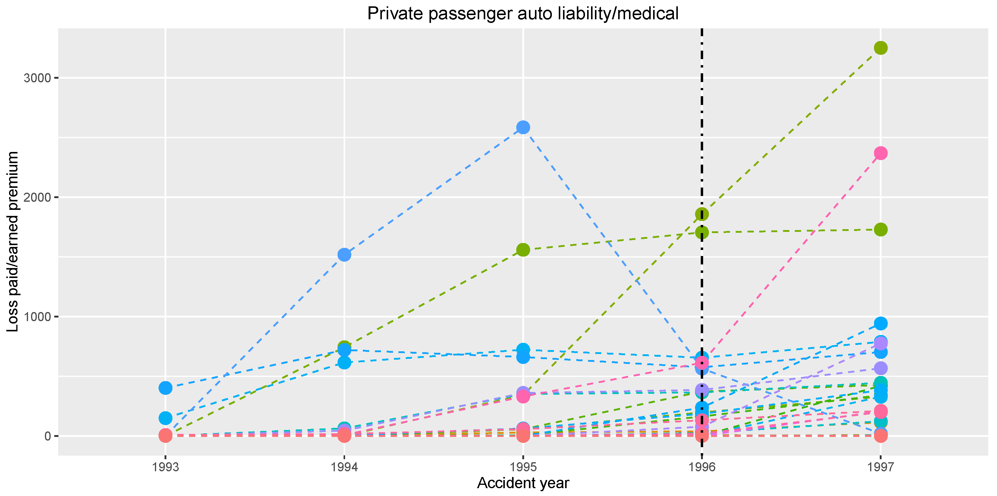Figure 6 graphically shows series of the normalized claim amounts.

The data are considered as panel data in the way that each insurance company corresponds to one panel, which is formed by the company’s yearly total claim amounts normalized by the earned premium. The length of the panel is quite short. This is very typical in insurance business, because considering longer panels may invoke incomparability between the early and the late claim amounts due to changing market or policies’ conditions over time.

We want to estimate a possible change in the normalized claim amounts occurring in a common year, assuming that the normalized claim amounts are approximately constant in the years before and after the possible change for every insurance company. Our change point estimator gives ${\widehat{\tau }}_{146}=9$ (i.e., year 1996) using the sequence of weights ${\left\{t^2\right\}}_{t=1}^{10}$ and $w\left(0\right)=1$, which corresponds to the increased values for the last observed year 1997 shown in Figure 6.

An interesting finding comes out, when one concentrates only on the second half of the observation period; see Figure 7. The shortening of the time window up to years 1993–1997 yields the same change position, i.e., year 1996.

Furthermore, the empirical cumulative autocorrelation function can be obtained. The correlation matrix is estimated as proposed in Section 5.1. The subsequence from the empirical cumulative autocorrelation function is obtained ${\left\{\widehat{r}\left(t\right)\right\}}_{t=1}^{10}=\{1.0,2.5,3.6,4.6,5.6,6.6,7.6,8.6,9.6,10.6\}$.

Dependent panels may be taken into account, and the presented work might be generalized for some kind of asymptotic independence over the panels or prescribed dependence among the panels. Nevertheless, our incentive is determined by a problem from non-life insurance, where the association of insurance companies consists of a relatively high number of insurance companies. Thus, the portfolio of yearly claims is so diversified, that the panels corresponding to insurance companies’ yearly claims may be viewed as independent, and neither natural ordering, nor clustering has to be assumed.

7. Results and Conclusions

The change point problem in panel data with a fixed panel size is considered in this paper. A possible occurrence of common breaks in panel means is estimated. We introduce the change point estimator without the boundary issue, meaning that it can estimate the change close to the extremities of the studied time interval. The consistency of the estimator is proven regardless of the presence/absence of the change in panel means under relatively simple conditions.

The simulation study illustrates that the proposed change point estimator behaves sufficiently well for small panel sizes, a relatively moderate number of panels and various errors’ dependence structures. The theoretical usage of the change point estimator is outlined for the estimation of the within-panel correlation structure and for the validity of the bootstrap procedures in hypothesis testing. Finally, the proposed method is applied to an actuarial problem, for which the change point analysis in panel data provides an appealing approach.