1. Introduction
General interest towards non-parametric thinking has increased over the last few years. One example is density estimation under shape constraints instead of requiring the membership of a parametric family. Here, a particularly robust alternative to parametric tests is provided by searching for the best fitting log-concave density. Another example is the mean excess plot that aims at distinguishing light and heavy tails.
Throughout the paper, we consider i.i.d. random variables with common distribution F having density f and tail . Then, X is (right) heavy-tailed if for all and light-tailed otherwise. The density f is log-concave, if , where is a concave function. If is convex, then f is log-convex. This paper aims to illustrate that light-tailed asymptotic behaviour is associated with log-concave densities. Likewise, log-convexity seems to be connected to heavy-tailed behaviour. One can use the connection to assess potential heavy-tailedness by searching for patterns that are typically present among distributions with log-concave or log-convex densities.
Log-concavity is a widely studied topic in its own right [
1,
2]. There also exists substantial literature regarding its connections to probability theory and statistics [
3,
4]. Several papers concentrate on the statistical estimation of density functions assuming log-concavity [
5,
6]. This is due to the fact that log-concavity provides desirable statistical properties for estimators. For instance, maximum likelihood estimation becomes applicable and the estimate is unique. The topic is discussed in detail in the beginning of [
7]. Unfortunately, much less emphasis seems to be put on verification of the log-concavity property itself. Specifically, it seems to be relatively little studied if it is feasible that the sample be generated by a log-concave distribution. See, for example [
8,
9].
A distribution with a log-concave density
f is necessarily light-tailed. In contrast,
f is log-convex in the tail in the standard examples of heavy tails such as regular variation, the lognormal distribution and Weibull case
with
. An important class of heavy-tailed distributions are the subexponential ones defined by
. The intuition underlying this definition is the principle of a single big jump:
is large if one of
is large, whereas the other remains typical. This then motivates
being close to 1. In contrast, the folklore is that
contribute equally to
with light tails. We are not aware of general rigorous formulations of this principle, but it is easily verified in explicit examples like a gamma or normal
F (see further below) and, for a large number of summands rather than just 2, it is supported by conditioned limit theorems (see e.g., ([
10] (VI.5))). However, it was recently shown in [
4] that these properties of
R hold in greater generality and that asymptotic properties of the corresponding conditioned random variable
provide a sharp borderline between log-convexity and log-concavity.
In this paper, we provide a wider perspective in terms of both sharper and more general limit results and of the usefulness for visual statistical data exploration. To this end, we propose a feature based nonparametric test. It can be used as a visual aid in identification of log-concavity or heavy-tailed behaviour. It complements earlier ways to detect signs of heavy-tailedness such as the mean excess plot [
11]. Further tests based on probabilistic features have been previously utilised in e.g., [
12,
13,
14].
2. Background
A property holds
eventually, if there exists a number
so that the property holds in the set
. Standard asymptotic notation is used for limiting statements. These and basic properties of regularly varying functions with parameter
α, denoted RV(
α), can be recalled from e.g., [
15].
We note that the principle of a single big jump relates to the fact that joint distributions of independent random variables concentrate probability mass to different regions. For example, a distribution with tail function
satisfies
for
and
for
, as
. We refer to [
16,
17,
18,
19] for related work in this direction. It is shown in Lemma 1.2 of [
4] that log-concavity or log-concavity of the density is closely related to the occurrence of the principle of a single big jump. A further observation in this direction is the following lemma. It states that contour lines of joint densities of independent variables behave differently for log-concave and log-convex densities, and thereby leads naturally to different concentrations of probability mass of joint densities (recall that a contour line corresponding to a value
of joint density
is the set of points in the plane defined as
).
Lemma 1. Suppose
and
are i.i.d. unbounded non-negative random variables. Assume further that they have a common twice differentiable density function
f of the form
where
h is a strictly increasing function.
If f is log-concave (log-convex), then, for any fixed , there exists a convex (concave) function defining a contour line of corresponding to p such that for all .
Lemma 1 implies that log-convex and log-concave densities cause maximal points of joint densities to accumulate into different regions in the plane. Log-convex densities tend to put probability mass near the axis, while log-concave densities have a tendency to concentrate mass near the graph of the identity function. The exponential density is the limiting case where all contour lines are straight lines. More generally, for , where is an integration constant, the contour lines are circles for , straight lines for , and parabolas for .
3. Theoretical Results
The emphasis of the paper is on the mathematical formulation of the connection between log-convexity and the principle of a single big jump. However, some additional theoretical results are provided concerning convergence rates of the conditional ratio defined in Equation (
3). These rates, or estimates for the rates, are obtained in some standard distribution classes. Their proofs are mainly based on sharp asymptotics of subexponential distributions obtained in [
20,
21,
22]. Recall that some main classes of such distributions are RV
, meaning regularly varying ones, where
with
and
are slowly varying, Weibull tails with
for some
, and lognormal tails which are close to the case
of
for
and some
; we refer in the following to this class as
lognormal type tails.
3.1. Convergence Properties
Define the function
by
It can be viewed as a generalisation of the function
considered in [
4] and has the same interpretation as in the case with densities: if both
and
contribute equally to the sum
, then
g should eventually obtain values close to 0; similarly, if only one of the variables tends to be the same magnitude as the whole sum, then
g is close to 1 for large
d. Note also that
g is scale independent in the sense that
for all
. Due to this property, two or more samples can be standardised to have, say, equal means in order to obtain graphs on the same scale.
In Proposition 1, sharp asymptotic forms of g are exhibited in some classes of distributions.
Proposition 1. The following convergence rates hold for
g defined in Equation (
3).
Let
X be RV
with
, eventually decreasing density
f. Then,
Let
X be Weibull distributed with
. Then,
Let
X be of lognormal type. Then,
Remark 1. In the case of Weibull and lognormal distributions, the implication is that
converges to 1 at a larger rate than their associated hazard rates tend to zero. In addition, inspection of the proof shows
This implies that the actual convergence rate can not be substantially larger than in the regularly varying case, where the leading term is explicitly identified.
The light-tailed case appears to be more difficult to study than the heavy-tailed case. Difficulty arises mainly from the lack of good asymptotical approximations for probabilities of the form when decays much faster than . Interestingly, the full asymptotic form of g can be recovered in the special case of the normal distribution if we allow X to obtain negative values.
Proposition 2. Suppose that
X is normally distributed with
and
. Then,
The following theorem can be used to assess if a sample is coming from a source with log-concave density. It can be seen as a natural continuation as well as a generalisation to [
4].
Theorem 1. Assume the density
f is twice differentiable and eventually log-concave. Then,
Similarly, if
f is eventually log-convex, then
4. Statistical Application: Visual Test
Suppose
is a sequence of i.i.d. vectors whose components are also i.i.d. One can formulate the empirical counterpart of Quantity (
3) by setting
where
and
is the indicator function of the event
A.
Remark 2. Equation (
9) requires as input a two-dimensional sequence of random variables. One can form such a sequence from a real valued i.i.d. source
using any pairing of the
. Obvious examples are to take
to take the set
as all pairings of the
or as a randomly sampled subset of these
pairings. If the data is truly i.i.d, this should not have any effect on the outcome.
4.1. Examples and Applications
A graph of
as function of
d can be used to determine if the data support the density being log-concave or light-tailed behaviour. According to Theorem 1, the graph should then stay below
.
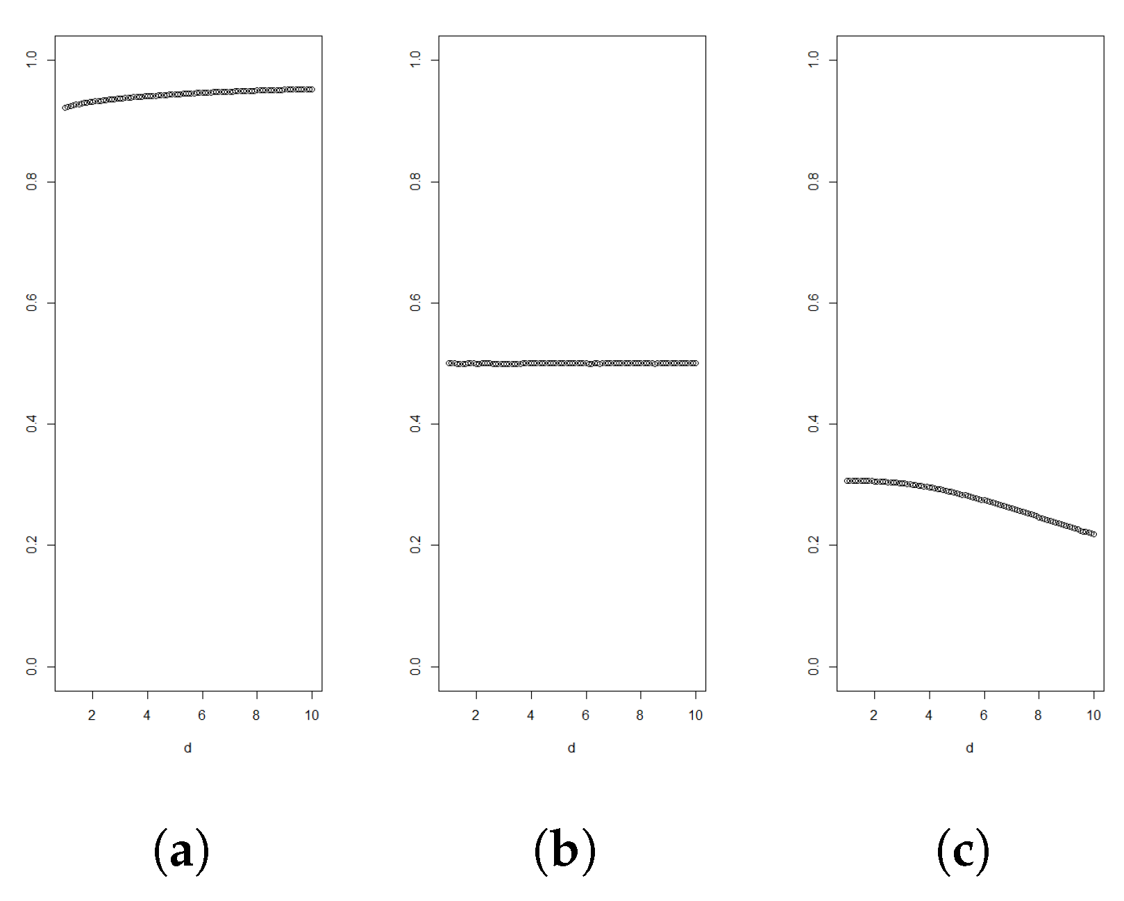
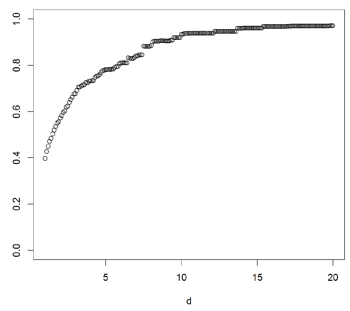
Figure 1,
Figure 2,
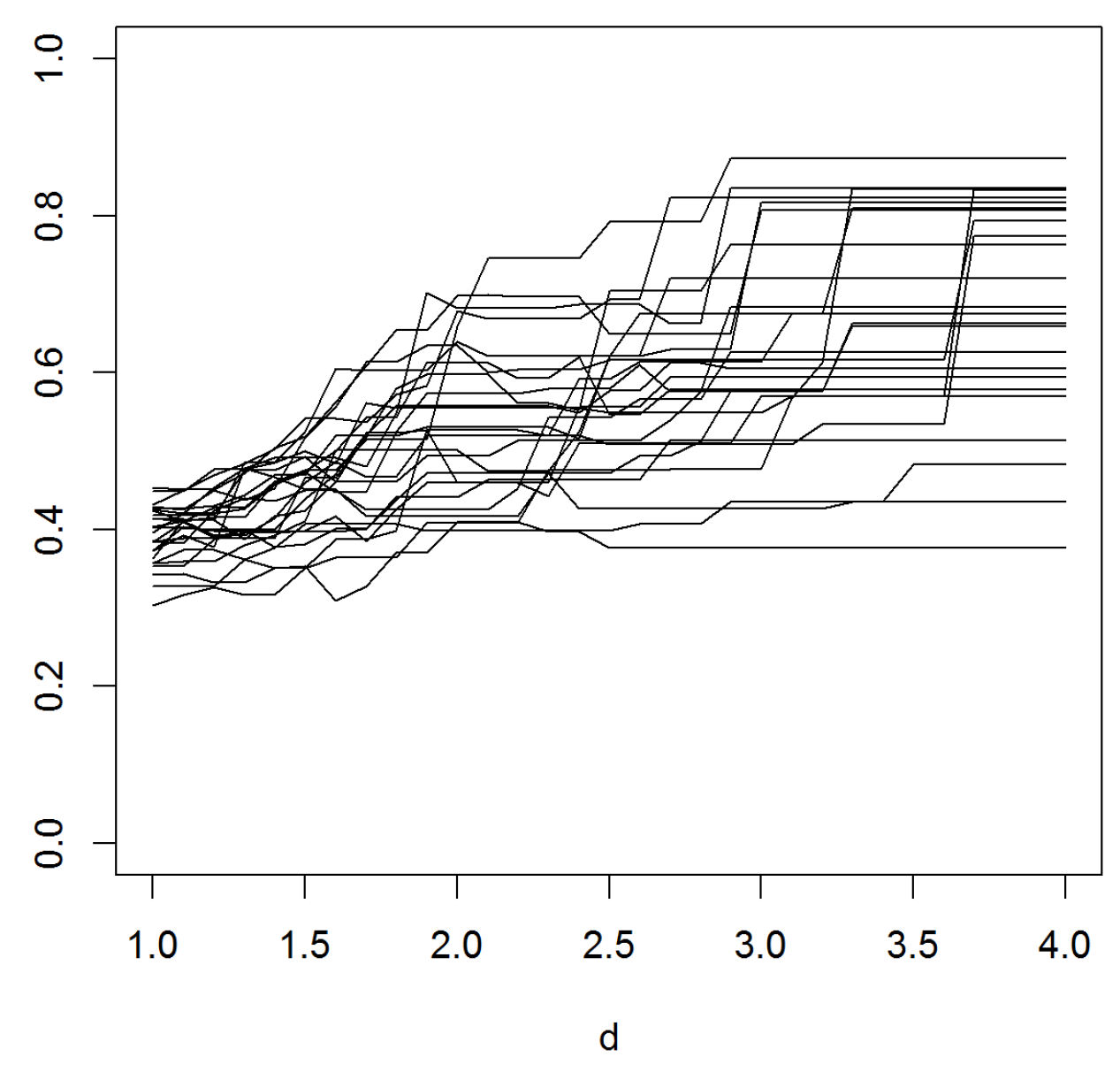
Figure 3 and
Figure 4 illustrate such graphs using experimental data.
The test method is visual. A similar idea has been used at least in the classical mean excess plot, where one visually assesses if the tail excess in the sample points is increasing at the level, as is the case for heavy tails.
4.2. Finer Diagnostics
The idea of plotting as a function of d was introduced as a graphical test for distinguishing between heavy-tailed and log-concave light tailed distributions. It seems reasonable to ask if the plot can be used for finer diagnostics, in particular to further specify the tail behaviour of F when F was found to be heavy-tailed. Such an idea would be based on the rate of convergence of to 1.
To gain some preliminary insight, we simulated
and
i.i.d pairs of r.v.’s
from an
F which was either RV(1.5), lognormal(0,1) or Weibull(0.4). The results are in
Figure 5 as plots of
, with three runs in each subfigure.
A first conclusion is that a sample size of is grossly insufficient for drawing conclusions about the way in which approaches 1—random fluctuations take over long before a systematic trend is apparent. The sample size is presumably unrealistic in most cases, but even for this, the picture is only clear in the RV case. Here, seems to have a limit c, as it should be, and the plot is in good agreement with the value 2.4 = of c predicted by Proposition 1.
Whether a limit exists in the lognormal or Weibull case is less clear. The results of Proposition 1 are less definite here, but, actually, a heuristic argument suggests that the limit
c should exist and be
. To this end, let
be the order statistics. According to subexponential theory (see, in particular, [
25]),
are asymptotically independent given
, with
having asymptotic distribution
F and
being of the form
with
, and
E as in the proof of Proposition 1. For large
d, this gives
In the lognormal or Weibull case, one has and so . Taking expectations gives the conjecture.
For the Weibull,
, and the
part of
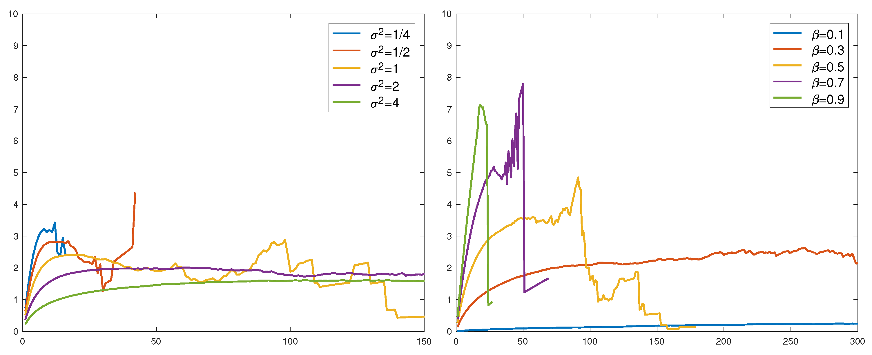
Figure 5 is rather inconclusive concerning the conjecture. We did one more run with
over a range of parameters (the variance
of
for the lognormal and
β for the Weibull). All
were normalized to have mean 1 so that the conjecture would assert convergence to
. This is not seen in the results in
Figure 6. Large values of
and small values of
β could appear to give convergence, but not to 2.
It should be noted that the heuristics give the correct result in the RV case. Namely, here we can take
and
. This easily gives
so that Quantity (
10) is approximately
, as rigorously verified in Proposition 1.
The overall conclusion is that the finer diagnostic value of the method is quite limited, and restricted to RV and sample sizes which may be unrealistically large in many contexts.
5. Proofs
Proof of Lemma 1. Suppose
h is concave and
. The contour line corresponding to value
p is formed as the set of points
that satisfy
, or equivalently
For any such pair
one can solve Equation (
11) for
y to obtain
Firstly,
is convex as the inverse of an increasing concave function. Secondly, the composition of an increasing convex function and a convex function remains convex. Thus, as a function of
x, Expression (
12) defines a convex function when
. Thus, one can define
.
If h is convex, the proof is analogous. ☐
The following technical lemma is needed in the proof of Proposition 1. It applies to Pareto, Weibull and lognormal type distributions. Indeed, condition (
13) follows from Proposition 1.2; (ii) of [
21] and further needed assumptions are easily verified apart from strong subexponentiality, which is known to hold in the mentioned examples.
Lemma 2. Suppose
and
are non-negative i.i.d. variables with a common density
f, where the hazard rate
is eventually decreasing with
. Assume further that
If in addition
, then
Proof. Equality (
13) implies subexponentiality of
. Writing
and observing that the nominator on the right-hand side is of order
proves Equation (
14) since
by subexponentiality.
On the other hand, writing
gives
Since we know from Equation (
16) that the leading term tending to zero must be
, Equation (
15) holds. ☐
Proof of Proposition 1. Suppose
X is regularly varying with index
α. In light of Lemma 2, we only need to establish
The contribution to the l.h.s of Equation (
17) from
is of order
for any
and
. Thus, it can be neglected. We are left with estimating
We will bound this quantity from above and below, assuming .
Now, given
,
is approximately distributed as
for large
x where
. Hence, dominated convergence gives
Here, the error terms and are of order . The latter error comes from Taylor expansion of function around point . The fact that f is assumed eventually decreasing guarantees that , when .
Secondly, for the lower bound, we have that
As before, we get
for error terms
and
of order
.
Repeating the argument with arbitrarily small
and combining the upper and lower estimates allows one to deduce
as
, which proves the claim.
Suppose then that
X is Weibull distributed. Now assumptions of Lemma 2 are satisfied with
. Since
for some
depending on
α, we only need to find the order of
In fact, proceeding similarly as in the regularly varying case, it can be seen that Quantity (
18) equals
It is known that
, where
, converges in distribution to a standard exponential variable, as
. Because
, it holds for
that
(the interchange of expectation and convergence is justified by dominated convergence). In addition, the same error term can be used for any
y.
Thus, Quantity (
19) can be written as
Now, using the definition of
from Lemma 2 with Equality (
15), we get
and
since
Equation (
20) follows from the fact that conditionally to
, all probability mass concentrates near small values of
.
Gathering estimates and using Equation (
14) of Lemma 2 yields
This shows Equation (
4), and Equation (
5) can be obtained using similar calculations with
. ☐
Proof of Proposition 2. Note first that
and
are independent in the normal case. Denote
so that
. Let
be the mean excess function of
Z (inverse hazard rate). It is then standard that
is of order
and that
converges in distribution to a standard exponential. Writing
it follows in the same way as in the proof or Proposition 1 that the r.h.s. of Equation (
21) is
. This proves the claim. ☐
Proof of Theorem 1. Suppose
f is log-concave and twice differentiable. Since
it suffices to show that, for a fixed
z, it holds that
where
In fact, by symmetry, one only needs to show
It is known from the proof of Proposition 2.1 of [
4] that
is increasing in
. Since
is non-negative and integrates to one over interval
, there exists a number
such that
when
and
when
. Therefore,
which proves Inequality (
23). Generally, if
f is log-concave and twice differentiable in the set
, then
is increasing in the set
. The difference from the presented calculation vanishes in the limit
, and thus Inequality (
7) holds.
If
f is eventually log-convex, the proof is analogous and Inequality (
8) holds. ☐


