A Discussion of a Risk-Sharing Pension Plan

Abstract

I show that risk-sharing pension plans can reduce some of the shortcomings of defined benefit and defined contributions plans. The risk-sharing pension plan presented aims to improve the stability of benefits paid to generations of members, while allowing them to enjoy the expected advantages of a risky investment strategy. The plan does this by adjusting the investment strategy and benefits in response to a changing funding level, motivated by the with-profits contract proposed by Goecke (2013). He suggests a mean-reverting log reserve (or funding) ratio, where mean reversion occurs through adjustments to the investment strategy and declared bonuses. To measure the robustness of the plan to human factors, I introduce a measurement of disappointment, where disappointment is high when there are many consecutive years over which benefit payments are declining. Another measure introduced is devastation, where devastation occurs when benefit payments are zero. The motivation is that members of a pension plan who are easily disappointed or likely to get no benefit, are more likely to exit the plan. I find that the risk-sharing plan offers more disappointment than a defined contribution plan, but it eliminates the devastation possible in a plan that tries to accumulate contributions at a steadily increasing rate. The proposed risk-sharing plan can give a narrower range of benefits than in a defined contribution plan. Thus it can offer a stable benefit to members without the risk of running out of money.

1. Introduction

Risk-sharing pension plans offer a middle ground between the extremes of defined benefit (DB) and defined contribution (DC) pension plans. They don’t promise a certain level of pension at retirement like DB plans, but neither do they promise something that they may not deliver. They don’t give members control over their own investment strategy like DC plans, but neither do they require members to be financial experts. Instead, they try to pay a stable pension to the members. They try to give members an idea of what their pension may be in retirement, but an aim or target amount rather than a guarantee. And they try to actively maintain the sustainability of the plan to adverse investment returns, by adjusting one or more of the investment strategy, benefits and contributions to be paid.

I discuss a model risk-sharing pension plan that adjusts only the investment strategy and retirement benefits. It is closer to a DC plan than a DB plan. In the risk-sharing plan, the retirement benefits are the accumulated value of the contributions. The plan reduces retirement benefit volatility to the plan members, paying a more stable benefit to its members than under a DC plan. It does not require additional contributions to make good a funding deficit. Instead, the benefits paid and investment strategy adjust so that the funding level is self-correcting. Adjusting the investment strategy means adjusting the level of investment risk taken by the plan. Moreover, the structure of the plan is highly flexible. By changing the parameters of the plan, the amount of benefit volatility experienced by different generations of members can be adjusted.

Although DB plans are currently in decline, they have some very appealing features for their members. A retirement “defined benefit” income or lump sum is promised to the plan members without regard to the achieved investment return. This is very attractive to the membership since they are insulated from the ups and downs of investment returns. However, the adverse consequence is that a DB plan can require large cash injections from its sponsoring employer. If the sponsor does not make the cash injections, then the plan may have to wind up and secure whatever fraction of the promised benefits it can for its members. In recent years, poor equity returns and low interest rates have resulted in many DB plans being underfunded [1]. As a result, many employers are closing down their DB plans and replacing them by DC plans [2].

In contrast, DC plans are in the ascendancy in countries such as the UK and USA. They have some very appealing features for the employer who sets them up on behalf of their employees. DC plans require no unexpected contributions to make good a funding deficit. This means that the employer has no uncertainty about their contribution rate to a DC plan, unlike in a DB plan. Typically, members and the employer pay in contributions which are invested in the financial market. The accumulated value of their contributions, which varies directly with the investment return achieved, is the value of the benefit paid to a member at their retirement date. There are no guarantees as to the amount of the retirement benefit, unless a financial guarantee is purchased. Thus members are exposed to the full volatility of their investment choices. If returns are much lower than expected, members may question the value of saving for retirement and not save enough for their retirement. Moreover, in DC plans the member must choose the investment strategy, although many people are financially illiterate [3] and do not consult a financial advisor ([Figure 325], [4]).

They are other types of pension plans, such as collective DC (CDC) plans. They are a type of risk-sharing plan, which can adjust the benefits paid to members in response to achieved investment returns. If annuities are paid as a benefit from a CDC plan, then the benefits can also be adjusted in response to mortality experience. The Dutch hybrid pension plans [5] can be considered as the latter type of CDC plan.

Plans with inter-generational risk-sharing, such as CDC plans and other risk-sharing plans, have been shown to be welfare-improving, compared to the individually optimal lifecycle strategy [6,7]. This is when measuring welfare using an expected utility-of-consumption framework, and maximizing utility across all generations. Inter-generational risk-sharing plans have higher and smoother consumption patterns, averaged across generations, than in a pure DC plan. More generally, risk-sharing in pension plans is discussed in Pugh and Yermo [8] and Blommestein et al. [9], both in terms of types of risk and who bears each risk. For example, in both DB and cash-balance plans the sponsoring employers bear the investment risk, whereas the members bear this risk in DC plans and in the plan analyzed here. Another example are conditional indexation plans: they share investment risk between the sponsor and the members, and the members’ basic benefit is guaranteed by the sponsor but benefit increases are not.

Closely related to the idea of risk-sharing plans are participating policies, which are contracts issued by insurance companies. Participating policies typically increase contributions annually at the risk-free rate, and thus provide a minimum guarantee of the benefit paid at retirement. Briys and De Varenne [10] study a model participating policy, focusing on the maturity value of the policy. Other studies including the minimum guarantee are Barbarin and Devolder [11], Graf et al. [12], Grosen and Jørgensen [13], Hieber et al. [14]. Guillén et al. [15] analyze a policy that was launched by a Danish insurance company. The policy smooths investment returns over the contract duration, but does not guarantee a minimum investment return. In these new contracts, there is no direct or indirect inter-generational investment risk-sharing. Baumann and Müller [16] propose a pension plan in which benefits are increased by the risk-free rate plus or minus a proportion of the funding level above or below a desired funding level. They find the static investment strategy that maximizes the discounted expected utility of employees averaged over all generations. They find that their proposed plan increases the risk tolerance and the expected utility of the retirement benefits. Analyses of different surplus appropriation schemes in participating policies are provided by Bohnert and Gatzert [17] and Zemp [18].

The risk-sharing pension plan that I study changes explicitly both the accumulation of contributions and the investment strategy in response to changes in a notional funding level. Thus it is not like a Dutch-style plan, nor a typically considered CDC plan in the literature, in which there is no explicit adjustment to the investment strategy. It is an adaptation of the scheme proposed by Goecke [19], which he proposed in the context of a with-profits contract. Unlike many with-profit contracts, there are no investment guarantees in Goecke’s scheme, and hence there is no need for an insurance company to financially underwrite the proposed contract. Thus Goecke’s scheme could be considered as a type of CDC plan, since the policyholders collectively bear all of the risk. However, Goecke [19] considers only a single generation of members, all of whom enter the contract at the same time with the same amount of money, and obtain the terminal value of the contract at the same time. In this paper, I analyze how the plan performs over time when there are regular withdrawals from its assets, which is not generally a consideration for with-profits contracts and was thus, unsurprisingly, not considered in Goecke [19].

The risk-sharing plan promises to increase the accumulated value of contributions each year in line with the expected return on assets, adjusted for the plan being over- or under-funded relative to a target funding level. Although the plan uses a notional funding level in its operation, benefits are not guaranteed. While the increase in the accumulation of contributions varies each year, the idea is that the annual variation in the accumulation increase is kept small. The notional funding level is simply a mechanism to determine the investment strategy and accumulation on the contributions at a selected time. The target funding level is fixed and its value helps to determine the spread of investment returns across generations.

The plan invests its money in line with a long-term strategic investment strategy, which would be chosen by the trustees or plan managers. However, if the plan is over-funded, then the investment risk of its strategy is increased (and correspondingly its expected investment return is increased). The opposite happens if the plan is under-funded: the investment risk is decreased. The two adjustments, to the accumulated contributions and the investment strategy, act to encourage the funding level back towards the target funding level.

I examine the robustness of the proposed risk-sharing pension plan from the viewpoint of individual members. I believe this is more appropriate for private pension plans than a social-planning viewpoint. Plans can fail because of what happens to one generation, regardless if they are expected to be a success averaged across all generations.

I focus on the actual retirement benefit payments made to members, as this is the ultimate purpose of the plan, rather than, for example, maximizing the expected utility derived from the payments. To do this, I examine the stability of the retirement benefit payments between generations of members and look at their distribution. Furthermore, in risk-sharing plans, it is inevitable that benefits have to be cut for some generations. However, the benefit cuts should not be too large between generations. A plan structure which means there is a high chance of members getting nothing is unlikely to succeed long-term in the marketplace. Similarly if the benefits decline year-on-year. For this reason, I calculate the probability of the plan’s assets being exhausted before all benefits have been paid, which I call devastation, and the probabilities of benefits declining year-on-year between generations, which I call disappointment.

I investigate (i) how changing the parameterization of the risk-sharing plan changes the range of benefits across generations; (ii) the retirement benefit stability across generations of members; (iii) disappointment, namely the frequency of runs of declining accumulation of contributions; and (iv) devastation, namely the chance of the plan exhausting its assets before all members have received their benefit.

I find that a suitably parameterized risk-sharing plan can offer a stable retirement benefit across generations. With a suitable choice of plan-specific parameters, it has a zero chance of running out of money before all members have retired, for the chosen financial market model. The downside is that members must expect that retirement benefits may decrease; there is no guaranteed minimum retirement benefit. While this is also seen in the DC plan, and many people are in DC plans, the risk-sharing plan members may compare themselves with other plan members and feel that they should get more each year.

2. Risk-Sharing Plan

The risk-sharing plan has the aim of paying a reasonable retirement benefit to its members, while maintaining the financial security of the non-retired members. Financial security is measured through the funding level of the plan, namely the ratio of the plan’s assets to its liabilities. The most attractive aspect is that each plan can be adjusted to the needs of the beneficiaries and sponsors, if any.

A target funding level is fixed and the plan’s managers seek to bring the funding level back to the chosen target, by adjusting the accumulated value of the members’ contributions and the investment strategy. The motivation is to maintain a cushion of assets as financial security for the non-retired plan members. This is done through applying the scheme of Goecke [19], and adapting it for use as an inter-generational pension plan.

Rather than pension plans that pay benefits, Goecke [19] studies with-profit contracts and introduces a mechanism for the smoothing of capital market returns in them. This involves changing the bonus declaration and the investment strategy in response to changes in the reserve ratio. A highly attractive property is that the log reserve ratio is mean-reverting to a fixed target log reserve ratio. As Goecke [19] studies with-profits contracts, which are held to the same maturity date, there is naturally no consideration of payments out. However, this must be allowed for in the risk-sharing plan as a pension plan is constantly paying out benefits to its retired members. Furthermore, I do not allow short-selling of any asset, which is a realistic assumption for a pension plan since the plan manager must act as a “prudent investor” [20].

2.1. Investment Strategy

Assume that time is measured in years. In the financial market, the plan can invest in a risky stock and a risk-free bond. The annual effective return over the time period $[n-1,n)$ on the risky stock is represented by the random variable $R_n>-1$, for $n=1,2,\dots$. For the risk-free bond, its annual effective return over the time period $[n-1,n)$ is the constant $r>-1$. The plan’s investment strategy at time n is represented by the proportion ${\pi }_n$ of assets invested in the risky stock, for each $n=0,1,2,\dots$. The proportion is determined through several elements.

One of the elements is a long-term strategic investment of $s^{\mathrm{LT}}$ in the risky stock. This can be decided by reference to the risk attitude of a typical member or, more realistically, the risk attitude of the trustees of the plan, a small group of people who run the plan in the interests of the members. An approach to deciding an investment strategy for a long-term investor like a pension fund is given in de Jong [21].

Another element of the strategy is positive or negative at time n, according to the funding level $F_n$ of the plan. The funding level is defined as the value of assets divided by the value of the liabilities, and it is formally defined in Section 2.3. If the plan is over-funded relative to a fixed target funding level $\overline{F}\ge 1$, then it invests more in the risky stock. The idea is that the plan can risk losing money by following a more risky investment strategy. The reverse is true when the plan is under-funded.

I impose the realistic investment constraints that the plan cannot short-sell the stock and neither can it invest more than 100% of its asset value in the stock. Taking these constraints into account, the total proportion of assets which are invested in the risky stock at time n, for investment over the period $[n,n+1)$ is

$${\pi }_n:=max\left\{0,min\left\{1,s^{\mathrm{LT}}+a\left(F_n-\overline{F}\right)\right\}\right\},$$

in which $a\ge 0$ is a constant called the investment risk adjustment that is chosen when the plan is set up, and $F_n$ is the plan’s notional funding level at time n. I state in Section 2.3 how the funding level is calculated. The higher the value of the constant a, the more sensitive is the strategy to over- and under-funding and hence the more volatile is the proportion invested in the risky stock.

2.2. Accumulation of Contributions

The members’ contributions are increased each year using a rate calculated via a pre-specified formula. Once each member’s retirement benefit, i.e., the accumulated value of their contributions, is paid to them as a lump sum on their retirement date, there is no more plan liability to that member.

The annual accumulation factor (AAF) granted on each member’s contributions at time n (i.e., for accumulation from time $n-1$ to time n) is

$$1+r+{\pi }_{n-1}(\mathbb{E}\left(R_n\right)-r)+\beta (F_{n-}-\overline{F}),$$

(1)

for $n=1,2,\dots$. The funding level $F_{n-}$ is the funding level just prior to any payment made at time n and it is defined in Section 2.3. The AAF adjustment $\beta \ge 0$ is chosen when the plan is set-up. There are two components to the AAF. The first is a stable return, $r+{\pi }_{n-1}(\mathbb{E}\left(R_n\right)-r)$, equal to the expected return on the assets for the current investment strategy.

The second component is a return, $\beta (F_{n-}-\overline{F})$, that is positive or negative according to the funding level of the plan relative to the target. The AAF is higher when the plan is over-funded relative to the target funding level, i.e., when $F_{n-}>\overline{F}$, as the plan can afford to grant higher accumulation factors. The higher value of the accumulated contributions acts to decrease the funding level when the plan is over-funded. The reverse happens when the plan is under-funded. The AAF adjustment β decrees the extent to which the AAF responds to situations of over- and under-funding; the higher the value of β, the greater the sensitivity. Notice that if $\beta =0$ then the AAF is not affected by deviations in the notional funding level from the target.

Here the funding level just prior to any payment out that is made at time n is used to calculate the AAF. If the funding level at time n was used then the AAF would have to be solved for implicitly, which makes the accumulation calculation more opaque to the members.

Let $B_n^{\left(k\right)}$ denote the value of the accumulated contributions of generation k at time n, for $n=1,\dots ,k$. It is calculated from the previous year’s accumulated value, $B_{n-1}^{\left(k\right)}$, and any new contributions as

$$B_n^{\left(k\right)}=B_{n-1}^{\left(k\right)}\left(1+r+{\pi }_{n-1}(\mathbb{E}\left(R_n\right)-r)+\beta (F_{n-}-\overline{F})\right)+C_n^{\left(k\right)},$$

in which $C_n^{\left(k\right)}\ge 0$ represents the new contribution made at time $n=1,\dots ,k-1$ by generation $k=2,\dots N$. As generation 1 retires at time 1, the only contribution that generation 1 makes is $B_0^{\left(1\right)}$ at time 0.

The retirement benefit depends directly on the investment strategy of the risk-sharing plan. This is not quite the same as in a DC plan, in which the contributions are increased at the rate of investment return on the assets. For example, a DC plan has its contributions increasing at the annual rate $r+{\pi }_{n-1}(R_n-r)$, i.e., with the actual return on the DC plan’s assets rather than with the expected return, as in the risk-sharing plans considered here.

2.3. Funding Level

The funding level of the risk-sharing plan is encouraged to move towards the target funding level. The AAF changes in response to deviations in the funding level, in order to bring the funding level back to the target value. Simultaneously, the investment strategy adjusts its investment risk-taking, lowering it if the plan is under-funded and otherwise raising it.

The funding level of the risk-sharing plan at time n is

$$F_n:=\frac{A_n}{L_n},$$

where $A_n$ is the value of the assets at time n. The value $L_n$ at time n, is a notional liability, since the plan does not guarantee to pay any benefit. The plan simply accumulates contributions. However, I regard the accumulated contributions as a notional deferred benefit. The notional liability is calculated assuming that the accumulated contributions at time n are increased at every subsequent year by the current expected return on the long-term investment strategy and discounted by the same expected return. In valuing the notional liabilities like this, the idea is that the retirement benefit is intended, but not guaranteed, to be the accumulated contributions that would be obtained from following the strategic long-term investment strategy and receiving the expected return on that strategy. Thus for N starting generations in the plan, of whom generations $n+1,\dots ,N$ will retire after time n,

$$L_n=\sum _{k=n+1}^N\left(B_n^{\left(k\right)}+C_n^{\left(k\right)}\right),$$

i.e., it is a notional liability to pay the current value of accumulated contributions to each currently non-retired generation, including their new contributions. The notional liability at time $n-$ includes the generation who are about to retire at time n, but accumulates their contributions at the expected, long-term strategic return over $[n-1,n)$ rather than the actual return, i.e.,

$$L_{n-}:=\left(1+r+s^{\mathrm{LT}}(\mathbb{E}\left(R_n\right)-r)\right)\sum _{k=n}^N{B}_{n-1}^{\left(k\right)}.$$

Accumulating the previous’s years contributions using the expected return on the long-term strategy is for two reasons: (i) to reflect the investment aim of the plan to invest in line with the long-term strategy; and (ii) to avoid the implicit equation involving $L_{n-}$ (through $F_{n-}$) that would arise if we used the AAF shown in (1).

3. Illustrations

3.1. Model Parameterization

For simplicity, I assume that the risky stock’s annual effective random returns $R_1,R_2,\dots$ are independent, lognormally distributed random variables each with location parameter μ and scale parameter $\sigma >0$. The continuously-compounded annual risk-free rate is denoted by the constant r. To parameterize the model, I used long-term returns. However, the risk-free bond return is “normalized” to 0% p.a. The reason for the normalization is to make it clear when members get a higher benefit from investing in the plan rather than investing all their money in the risk-free bond. The choice of the risk-free rate of 0% per annum means that, for example, a member who obtains a retirement benefit higher in value than their total contributions has done better than investing their contributions entirely in the risk-free asset. This corresponds to an average AAF which is greater than one.

The annual return on the S&P500 index over the years 1956–1999 is about 12% with an annual volatility of about 15%, based on the values in (Table 2.1, Hardy [22]). Over the same time period, annual 10-year US Treasury bond returns were around 7%1. This gives the S&P500 annual return to be about 5% above the 10-year US Treasury bond return.

To broadly mimic these historical long-term returns, set the financial market parameters to

$$r=0,\mu =0.0375,\sigma =0.15.$$

Then the mean annual return of the risky asset is $e^{\mu +0.5{\sigma }^2}-1\approx 0.05$ and its annual volatility is $\sqrt{e^{{\sigma }^2}-1}\times e^{\mu +0.5{\sigma }^2}\approx 0.15$.

The long-term strategic investment in risky stocks, $s^{\mathrm{LT}}$, is set to 80%. All the figures shown in the paper are based on 5000 simulations.

3.2. Comparison Plans

In most of the illustrations, I compare a selection of the risk-sharing pension plans to a pure DC plan, to understand better the advantages and disadvantages of the risk-sharing plan. I do not compare the plans to a DB plan, as the latter type of plan typically has a sponsoring employer who makes good any deficit and this makes a like-for-like comparison difficult. The DC plan follows exactly the long-term investment strategy of the risk-sharing plans, i.e., it invests the proportion $s^{\mathrm{LT}}$ of its assets in the risky stock, and the remainder in the risk-free asset. The strategy is rebalanced annually to this proportion. The benefit paid to a retiring member is the accumulation of that member’s contributions from time 0, accumulated at the actual achieved investment return. This results in a volatile benefit payment to all members over time: the benefit can decrease as well as increase in line with the cumulative investment return. The DC plan is always 100% funded, since the benefit promise is to pay the accumulation of the contributions.

In the preliminary investigation, I also compare the risk-sharing plans to a benchmark plan. In the benchmark plan, neither the investment strategy nor the AAF is adjusted for over- or under-funding, that is $a=0$ and $\beta =0$. Instead, the AAF equals the expected investment return each year based on the long-term strategic investment strategy $s^{\mathrm{LT}}$. This means that the benchmark plan is not a risk-sharing plan. Assuming that $s^{\mathrm{LT}}\in [0,1]$, then the AAF in year n in the benchmark plan is $\left(1+r+s^{\mathrm{LT}}(\mathbb{E}\left(R_n\right)-r)\right)$. I use this plan as a benchmark plan since it accumulates contributions at a constant rate, up to the time that it runs out of money (although it may not run out of money). It makes it a helpful reference line between the plots, and for this reason I keep it in the further investigation although I do not analyze it any more.

3.3. Preliminary Investigation

3.3.1. Simple Membership Profile

As a first look at the risk-sharing plan, I assume a simple membership. Each member pays a contribution of $1 at time 0, and nothing else. Thus $B_0^{\left(k\right)}=1$ for $k=1,2,\dots ,N$ and $C_n^{\left(k\right)}=0$ for $n=1,\dots ,k-1$ and $k=2,\dots ,N$. At the start, there are $N:=40$ members in the plan, the first of whom retires at time 1 (i.e., generation 1), the second of whom retires at time 2 (i.e., generation 2), and so on, until the Nth member retires at time N. This assumption is made to enable a straightforward comparison of outcomes between plans. In practice, members would be expected to pay contributions up to their retirement. Each member’s contributions are accumulated each year, until they are paid out at the member’s retirement date as a single lump sum. The final accumulated value of the contributions that is paid out to each retiring member is called the retirement benefit.

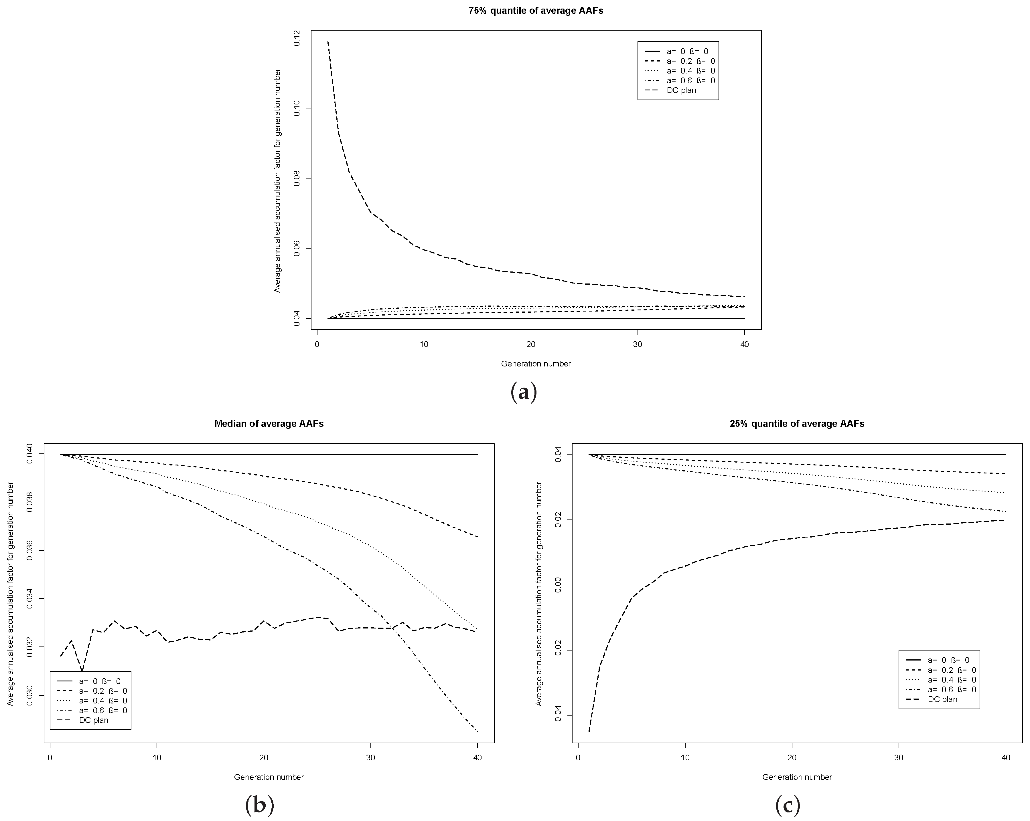
3.3.2. Plans Which Vary Only the Investment Strategy

Figure 1 illustrates quantiles of the (geometric) average AAF for plans which adjust only the investment strategy—through the parameter a—and not the accumulation factors. Rather than showing the accumulated contributions paid at retirement, the average AAF for each year is plotted. For example, if the AAF is $1.02$ for year 1, $1.03$ for year 2 and $1.05$ for year 3 then the average AAF is approximately $1.033={(1.02\times 1.03\times 1.05)}^{1/3}$. However, the average AAF of $1.033$ is displayed as $0.033$ in the figures.

Also shown in Figure 1 is a plot for a DC plan. In the DC plan, the proportion $s^{\mathrm{LT}}$ of its assets is invested in the risky stock, and the remainder in the risk-free asset. The strategy is rebalanced annually to this proportion. The retirement benefit paid to a member is the accumulation of that member’s contributions, accumulated at the actual achieved investment return. The solid black line shows the average AAF for the benchmark plan.

Examining the five plans (the benchmark plan, the DC and the three risk-sharing plans) at the three chosen quantiles, the risk-sharing plans have quite a smooth average AAF. The risk-sharing plans have a lower inter-quartile range of average AAFs than the DC plan. The lower the value of the parameter a in the risk-sharing plans, the lower is the inter-quartile range of the average AAF.

3.3.3. Plans Which Vary Only the AAFs

Next I consider risk-sharing plans which adjust only the AAFs—through the parameter β—and not the investment strategy. The 25%, 50% and 75% quantiles of the (geometric) average AAF is shown in Figure 2. Again, the DC and benchmark plan quantiles are also shown. It is observed than the risk-sharing plans do not have the same smooth average AAF as when the investment strategy is adjusted. As in the latter plans, the risk-sharing plans have a lower inter-quartile range of average AAFs than the DC plan, although the range is wider. The lower the value of the parameter β in the risk-sharing plans, the lower is the inter-quartile range of the average AAF. The figures suggests that the parameter β, which adjusts the annual accumulation factors, has a lesser effect on the AAFs than the parameter a, which adjusts the investment strategy.

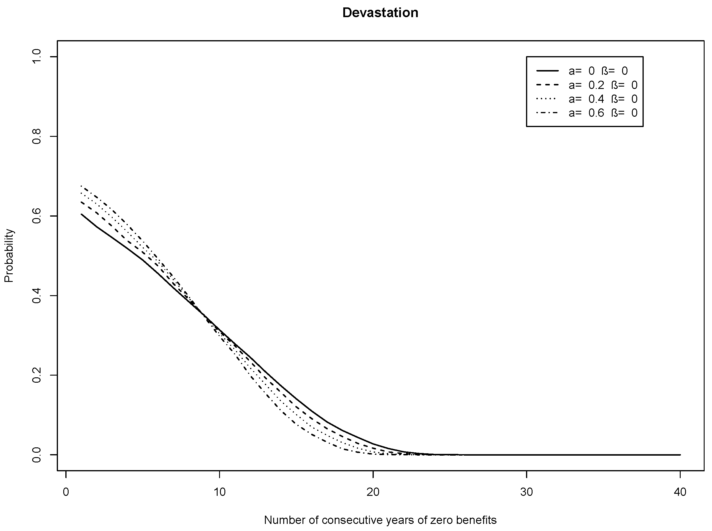
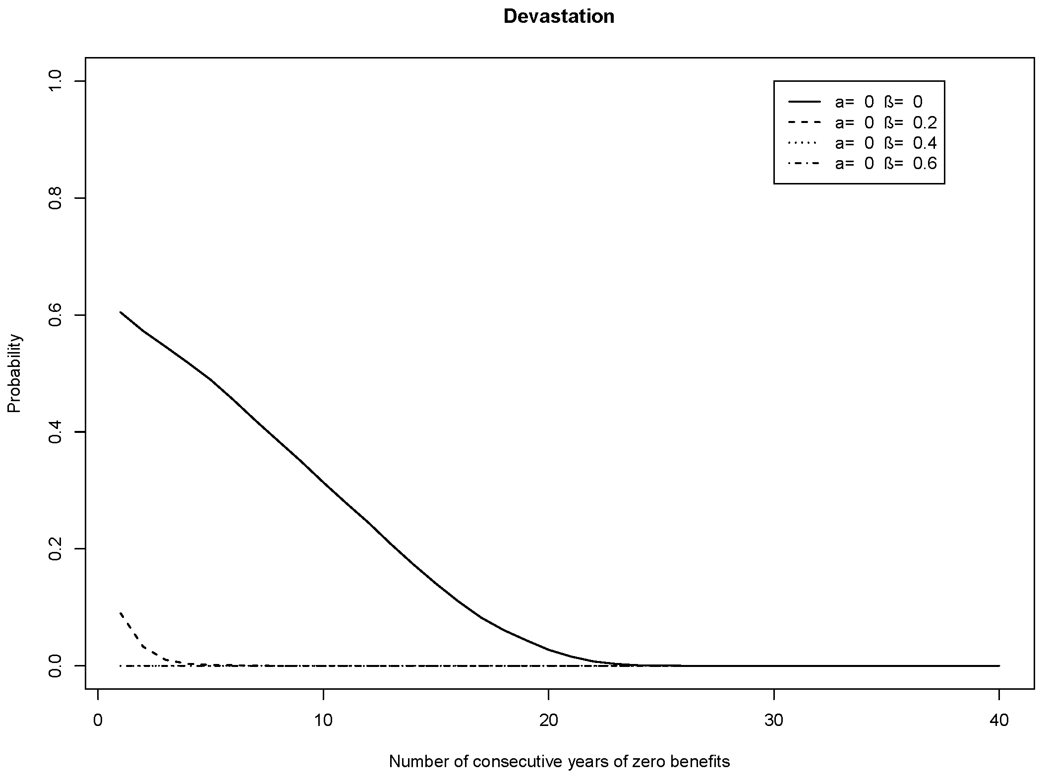
3.3.4. Devastation

Although the benchmark plan is promising to pay out a constant average AAF, of around $1.04$ per annum (which is displayed as $0.04$ in the figures), it may run out of money before the last generation has retired. To capture the catastrophic risk that a plan runs out of money before all members have retired, I introduce a measure of devastation. This counts the number of consecutive years in which retiring members receive zero retirement benefits. Doing this across all simulations, I can calculate the probability of two or more consecutive generations of members receiving zero retirement benefits, the probability of three or more consecutive generations receiving zero retirement benefits, and so on. As there is no sponsoring employer for any of the plans considered, then a probability of 30% of two or more generations receiving zero retirement benefits means that there is a 30% chance of the plan running out of money on or after the $(N-2)$th generation, where the Nth generation is the last generation to retire. The devastation measure is zero for the DC plan, since there is no risk-sharing, and it is therefore not shown in the devastation plots.

On the devastation measure, none of the plans in which only the investment strategy is adjusted perform particularly well (Figure 3). For these plans and the benchmark plan, there is a 60%–70% chance of the plan running out of money just before the last generation has retired (shown in Figure 3 as the left-most probabilities plotted for each plan). The risk-sharing plans have a higher probability of this event than the benchmark plan. However, this varies across the retirement times. There is around a 35% chance of all the plans running out of money just before the 31st generation has retired (shown in Figure 3 as the probabilities for 9 consecutive years of zero benefits). For generations retiring earlier than the 31st, the benchmark plan performs worse than the risk-sharing plans. For example, the benchmark plan has a 10% chance of running out of money just before the 25th generation has retired, and the corresponding probability for the considered risk-sharing plans is below 10% (shown in Figure 3 as the probabilities for 15 consecutive years of zero benefits). Risk-sharing plans with a lower value of the parameter β have a probability of running out of money which is closer to that of the benchmark plan.

Plotting the devastation measure for plans in which only the AAFs are adjusted, Figure 4 is obtained. Here, the difference of the risk-sharing plans from the benchmark plan is dramatic. The chance of the risk-sharing plans running out of money is significantly less than for the benchmark plan. The higher the value of the AAF adjustment β, the lower is this probability. However, it is important to note that although the members may receive something, the amount of their retirement benefits may be small.

3.3.5. Preliminary Findings

This preliminary investigation indicates the impact of the two adjustment factors. The average AAF is most sensitive to the investment strategy adjustment a. Choosing a positive value of a can reduce the inter-generational volatility of the retirement benefit, i.e., maintain a relatively steady increase in the AAF as the generations retire. However, the chance of the plan running out of money is most sensitive to the AAF adjustment β. Choosing a positive value of β can reduce the chance of the plan running out of money. For this reason, in the sequel, I examine plans in which both a and β are positive.

3.4. Further Investigation

Here I examine a different selection of the risk-sharing plans under a more realistic membership. In the selection of risk-sharing plans, both the adjustments a and β are positive. I also introduce a measure of disappointment that measures the year-on-year decline in the AAFs and their average. Examining the devastation measure is not meaningful for the membership, in which non-retired members make annual contributions. Due to the annual contributions, the plans do not run out of money.

The critical element to examine is the retirement benefit paid to the members, as this is the purpose of the plan. I look at the quantiles of the retirement benefit paid to each generation because this is important to an individual. I do not look at the expected retirement benefit across all generations. A beneficiary does not care if across all generations, the retirement benefit of Plan A is higher than Plan B, if they themselves get a lower benefit under Plan A than under Plan B.

Some questions to ask are: are the AAFs and their average high enough for each generation? Are they stable enough across the generations? Are earlier generations benefiting at the expense of the later generations, or vice versa? Through a numerical investigation, it is seen that the expected answers to these questions depend heavily on the choice of the three plan parameters: the investment strategy adjustment a, the AAF adjustment β and the target funding level $\overline{F}$.

3.4.1. Selected Risk-Sharing Pension Plans

I choose three plans which combine adjustments to both the benefits and the investments strategy, but which—for the chosen financial market model—do not result in the plan running out of money before all members have retired. I continue to keep the benchmark plan in, as a benchmark plan. The parameters of the plans are shown in

Table 1. Plan parameters for the risk-sharing plans.

Plan Type	Investment Risk Adjustment a	AAF Adjustment β
Benchmark plan	0	0
Risk-sharing	$0.2$	$0.2$
Risk-sharing	$0.2$	$0.4$
Risk-sharing	$0.4$	$0.2$
DC plan	N/A	N/A

.

3.4.2. Membership Profile

There are $N:=40$ generations at time 0, the first generation retiring at time 1, the second generation at time 2, and so on. The kth generation contributes $$(N+1-k)$ to the plan as an initial lumpsum payment at time 0, for $k=1,2,\dots ,40$. Additionally, each generation pays an annual lumpsum contribution of $1 at each integer time before their retirement time. Thus generation 1 pays only a lumpsum of $N at time 0, and nothing else until their retirement at time 1. Generation 2 pays a lumpsum of $$(N-1)$ at time 0, another contribution of $1 at time 1, and nothing else until their retirement at time 2. In the introduced notation, $B_0^{\left(k\right)}=N+1-k$ for $k=1,2,\dots ,N$, and $C_n^{\left(k\right)}=1$ for $n=1,\dots ,k-1$, for $k=2,\dots ,N$. The motivation is to represent the contribution profile of a more realistic membership. Moreover, by fixing the total amount of contributions made by each generation at $N, it makes the measure of disappointment introduced below more meaningful: members who contribute the same amount may feel that they should receive similar benefits.

The notional funding level of each risk-sharing plan is exactly equal to 100% at time 0.

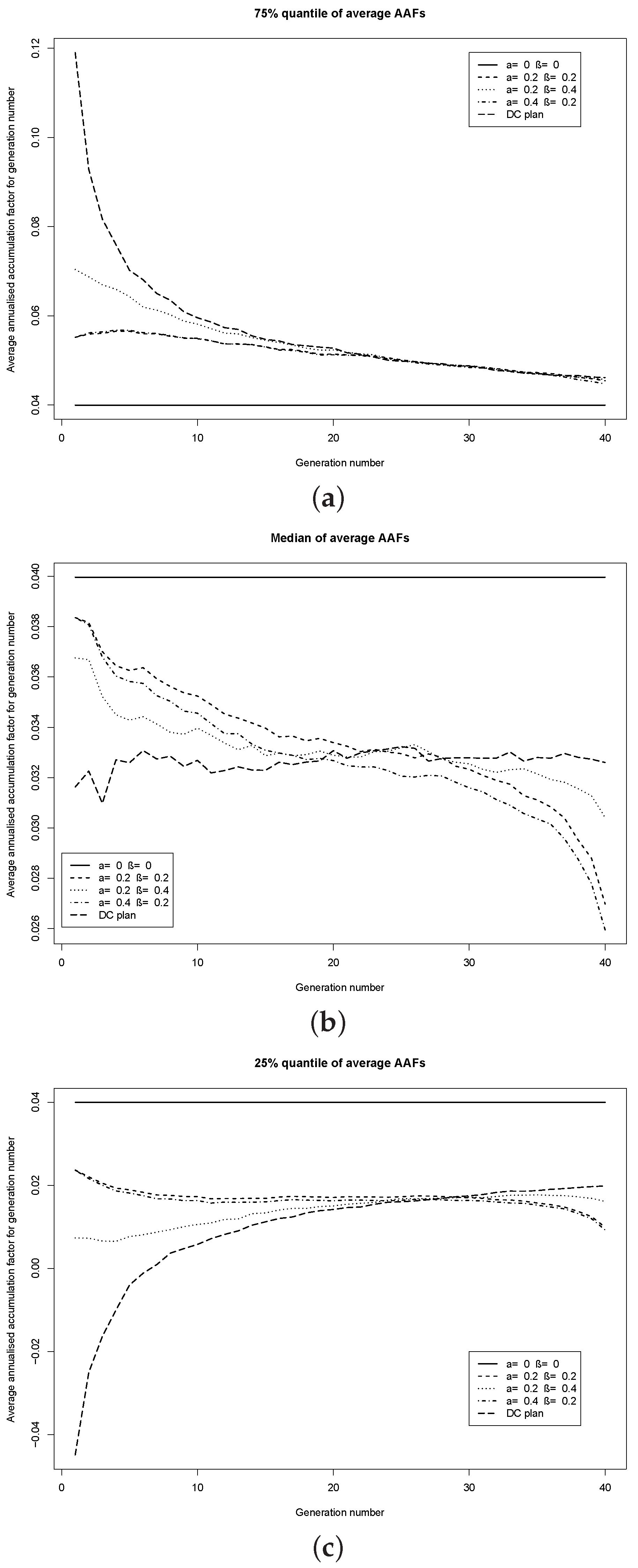
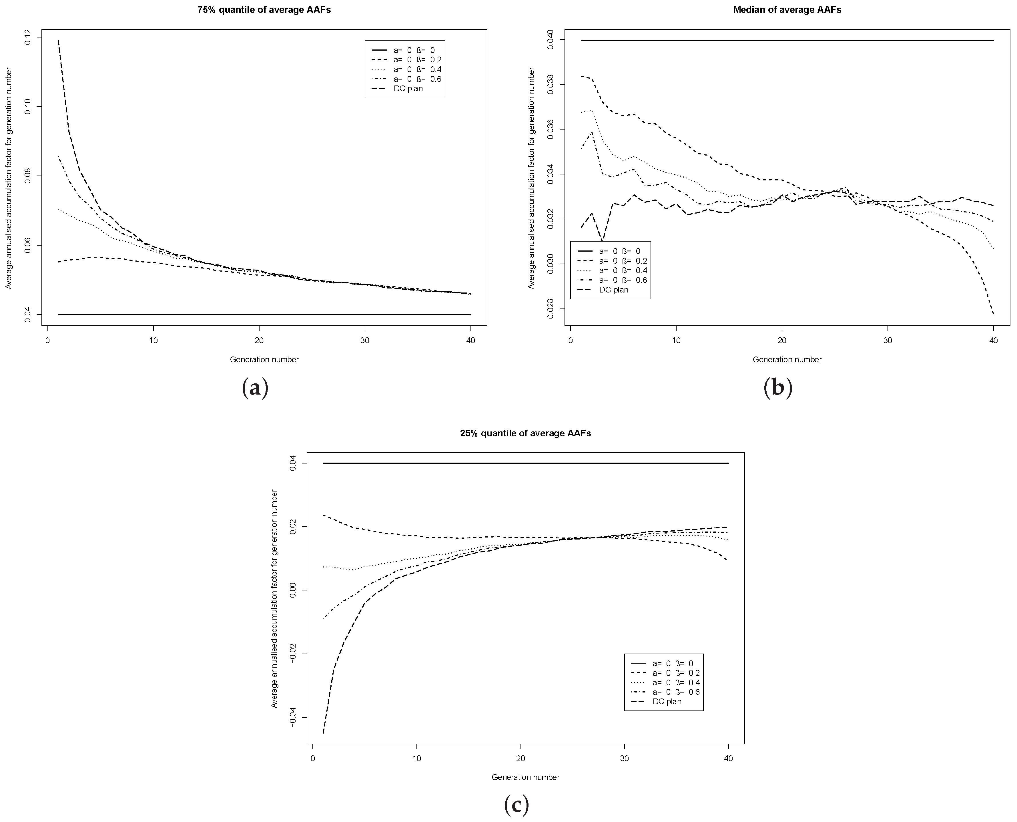
3.4.3. Quantiles of the Average AAF

Figure 5 shows the 25%, 50% (median) and 75% quantiles of the annualized average accumulation factor under the selected risk-sharing plans, the DC plan and the benchmark plan. The target funding level is $\overline{F}=100$% for the risk-sharing plans. It can be seen that up to, roughly, the 25th generation, the average AAF is more stable (i.e., has a lower inter-quartile range) under the risk-sharing plans than the DC plan. Past the 25th generation, the differences in inter-quartile range between the risk-sharing plans and the DC plan is not significant. The median average AAF has a decreasing trend as time increases for the risk-sharing plans, whereas it is flat for the DC plan.

The widest range of possible retirement benefits is with the DC plan. The earliest generations of the DC plan experience a huge range of possible benefits, although this declines with the investment period.

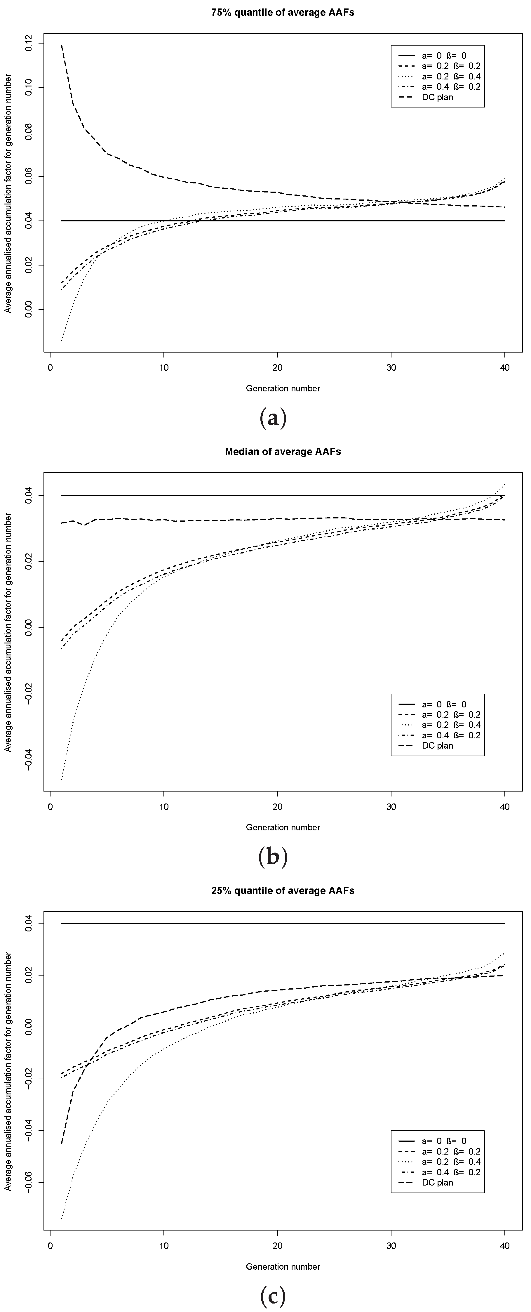
Increasing the target funding level to $\overline{F}=120$% for the risk-sharing plans, Figure 6 shows the same quantiles. Since the risk-sharing plans are only 100% funded at time 0, they attempt to reach the target funding level through reducing the AAFs (via the adjustment β) and reducing the investment in the risky stock (via the adjustment a). This is observed in the figures, as the average AAF is below one (shown in Figure 6 as negative values, since the figure displays the value of the average AAF minus one) for the earliest retiring generations, and becomes greater than one (shown in Figure 6 as positive values) for the later generations as the target funding level is attained. The average AAF remains more stable (i.e., has a lower inter-quartile range) under the risk-sharing plans than the DC plan, for generations up to, roughly, the 30th.

The shift in the median quantile, between Figure 5b and Figure 6b, is interesting. For the higher target funding level $\overline{F}=120$%, the median average AAF has an increasing trend as time increases for the risk-sharing plans. This is the opposite trend to the plans with a target funding level $\overline{F}=100$%. The conclusion is that the target funding level can be used to shift the investment gains from the latest retiring generations to the earliest retiring generations. The reason for this shift is that the plan attempts to build up a cushion of assets, to reach the target funding level $\overline{F}=120$%. This cushion comes at the expense of the earlier generations, who pay for it and hence who are more likely to receive a lower average AAF than the later generations.

The figures demonstrate the flexibility of the risk-sharing plan; the plan parameters allow us to adjust the average AAF quantiles (and hence the amount of retirement benefit) across the generations.

3.4.4. Analyzing Benefit Stability

Here I analyze the stability of the average AAFs across generations for each plan. Rather than looking at means, I try to capture the spread of the possible average AAFs through an inter-quantile range. Setting for generation $n=1,2,\dots ,40$,

$$\begin{array}{cc}\hfill {\mathrm{IQR}}_n& :=95\%\mathrm{average}\mathrm{AAF}\mathrm{quantile}\mathrm{of}n\mathrm{th}\mathrm{generation}\hfill \\ & -5\%\mathrm{average}\mathrm{AAF}\mathrm{quantile}\mathrm{of}n\mathrm{th}\mathrm{generation},\hfill \end{array}$$

Next I calculate the range of ${\left\{{\mathrm{IQR}}_n\right\}}_{n=1,\dots ,40}$ for each plan, namely

$$\mathrm{IQR}\mathrm{instability}:=\underset{n=1,2,\dots ,40}{max}\left\{{\mathrm{IQR}}_n\right\}-\underset{n=1,2,\dots ,40}{min}\left\{{\mathrm{IQR}}_n\right\}.$$

A plan with low instability should have an average AAF whose 5% to 95% quantile range does not change much between generations. However, this does not tell us whether the values in the range change between generations; a plan can have zero instability but generation 1 faces an average AAF in the range $[0\%,3\%]$, generation 2 in the range $[1\%,4\%]$, and so on. The disparity between the values of the average AAF is also important, so that a plan does not give highly negative increases to the earlier generations and highly positive increases to the later generations, or vice versa. To capture the latter, define

$$\begin{array}{cc}\hfill \mathrm{Quantile}\mathrm{inequity}& :=\underset{n=1,2,\dots ,40}{max}\left\{95\%\mathrm{average}\mathrm{AAF}\mathrm{quantile}\mathrm{of}n\mathrm{th}\mathrm{generation}\right\}\hfill \\ & -\underset{n=1,2,\dots ,40}{min}\left\{5\%\mathrm{average}\mathrm{AAF}\mathrm{quantile}\mathrm{of}n\mathrm{th}\mathrm{generation}\right\}.\hfill \end{array}$$

The lower the quantile inequity, the lower is the overall range of the average AAFs across all generations. This means that a plan with a low quantile inequity does not have the earlier generations benefiting at the expense of the later generations, or vice versa.

A narrower measure is the median inequity, which looks at the range of the median average AAF across all generations.

$$\begin{array}{cc}\hfill \mathrm{Median}\mathrm{inequity}& :=\underset{n=1,2,\dots ,40}{max}\left\{50\%\mathrm{average}\mathrm{AAF}\mathrm{quantile}\mathrm{of}n\mathrm{th}\mathrm{generation}\right\}\hfill \\ & -\underset{n=1,2,\dots ,40}{min}\left\{50\%\mathrm{average}\mathrm{AAF}\mathrm{quantile}\mathrm{of}n\mathrm{th}\mathrm{generation}\right\}.\hfill \end{array}$$

Table 2. Instability and inequity, across the generations for different target funding levels.

Plan Type	a	β	Target Funding Level $\overline{\mathit{F}}=100$%
			IQR Instability	Qu. Inequity	Median Inequity
Risk-sharing	$0.2$	$0.2$	$9.4\%$	$10.3\%$	$3.8\%$
Risk-sharing	$0.2$	$0.4$	$15.7\%$	$15.7\%$	$3.7\%$
Risk-sharing	$0.4$	$0.2$	$9.7\%$	$10.5\%$	$3.8\%$
DC	N/A	N/A	$40.7\%$	$40.7\%$	$3.3\%$
Plan Type	$\mathit{a}$	$\mathit{\beta }$	Target Funding Level $\overline{\mathit{F}}=\mathbf{120}$%
			IQR Instability	Qu. Inequity	Median Inequity
Risk-sharing	$0.2$	$0.2$	$9.5\%$	$12.1\%$	$4.4\%$
Risk-sharing	$0.2$	$0.4$	$14.9\%$	$19.4\%$	$8.9\%$
Risk-sharing	$0.4$	$0.2$	$9.5\%$	$12.2\%$	$4.6\%$
DC	N/A	N/A	$40.7\%$	$40.7\%$	$3.3\%$

shows the values of instability and inequity of the plans, for different target funding levels. Note that the values for the DC plan do not depend on the target funding level.

The risk-sharing plans have significantly lower values of IQR instability and quantile inequity than the DC plan. Thus, in terms of having a low range of possible average AAFs faced by different generations between the 5% and 95% quantiles, the risk-sharing plans perform well. The lowest measures are seen in the two plans with $\beta =0.2$. Looking further down the table, the IQR instability measures decline for the risk-sharing plans as the target funding level increases, but this is at the cost of the quantile inequity increasing. Thus while the 5%–95% inter-quantile range declines over all generations, the range of possible values that the average AAF can take increases.

Interestingly, the DC plan has the lowest median average AAF inequity. For the risk-sharing plans, the median inequity rises as the target funding level rises. This is the due to the plans starting with a funding level of 100%, and therefore being under-funded relative to the higher target funding levels considered. Earlier generations are granted lower AAFs as the plan attempts to reach the target funding level. Later generations gain from the lower payments out from the plan’s assets and the accumulated investment returns.

3.4.5. Disappointment

Although reducing the accumulated contributions is a integral part of the considered risk-sharing plans, perhaps some plan structures result in a higher chance of reductions in the accumulated value of contributions than others. If reductions occur too often, then it is possible that members will exit the plan. They will compare what they are getting with the recently retired members, and will be unhappy if they get a lower retirement benefit than them [23,24,25,26]. I call this member disappointment.

Member disappointment is related to disappointment aversion, which was introduced by Gul [27]. Ang et al. [28] develop a portfolio choice framework under disappointment aversion preferences, using a dynamic CRRA problem. Fielding and Stracca [29] analyze both loss and disappointment aversion, and find that stocks may disappoint in the long term.

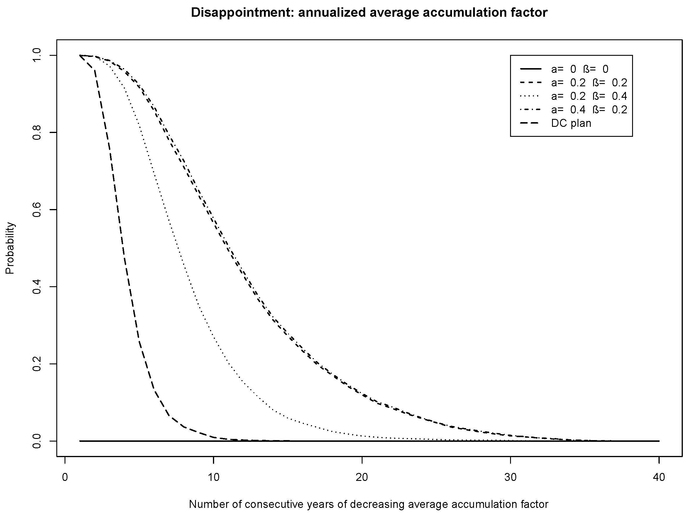
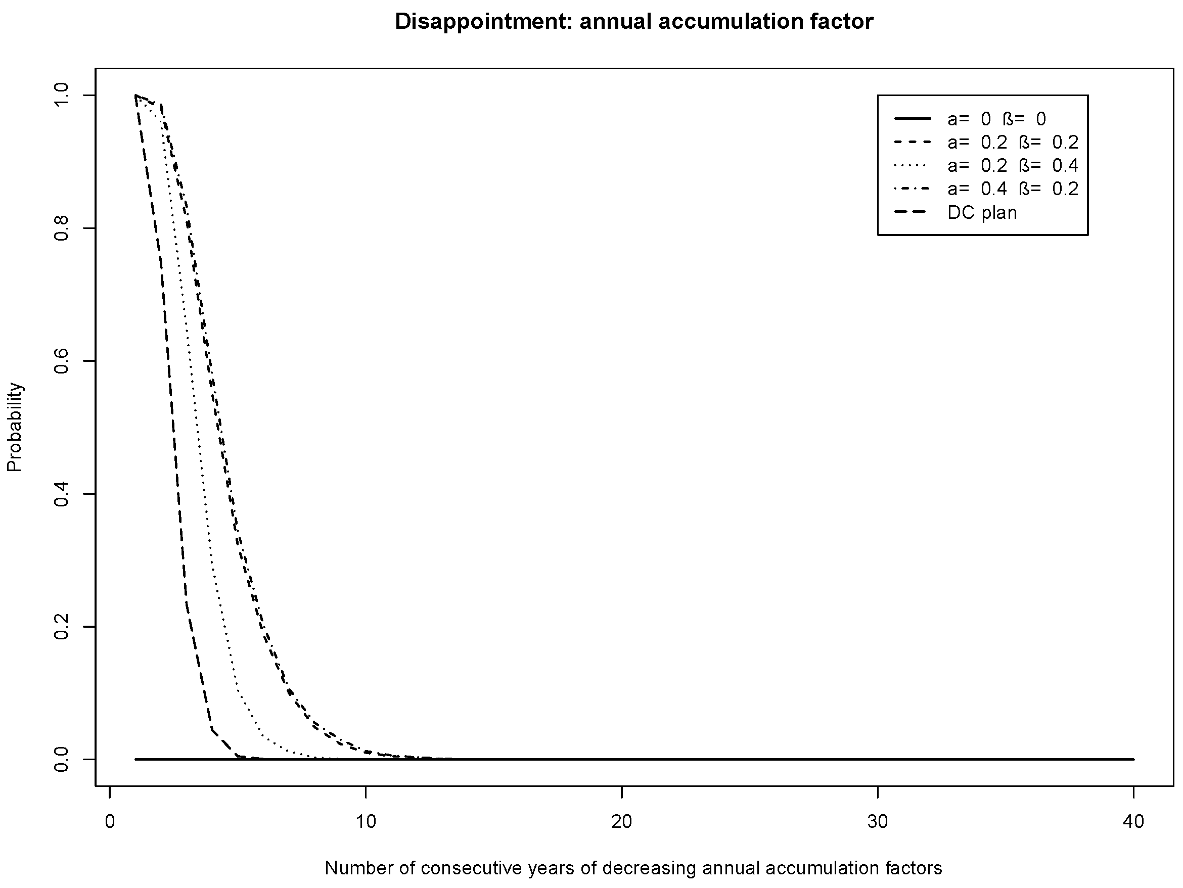
Here I introduce a way of trying to measure retiring members’ disappointment if their average AAF is less than the average AAF for the previous year’s retiring generation. To measure member disappointment over two consecutive years, in each simulation I count the number of runs of exactly two consecutive years in which the average AAF is strictly declining. Doing this across all simulations, I calculate the probability of having two consecutive years in which the average AAF is strictly declining. Using the same approach, I calculate the probability of having three consecutive years in which the average AAF is strictly declining. I repeat this for four consecutive years, five consecutive years and so on. The resulting probability can be used to see the frequency of runs of declining average AAFs.

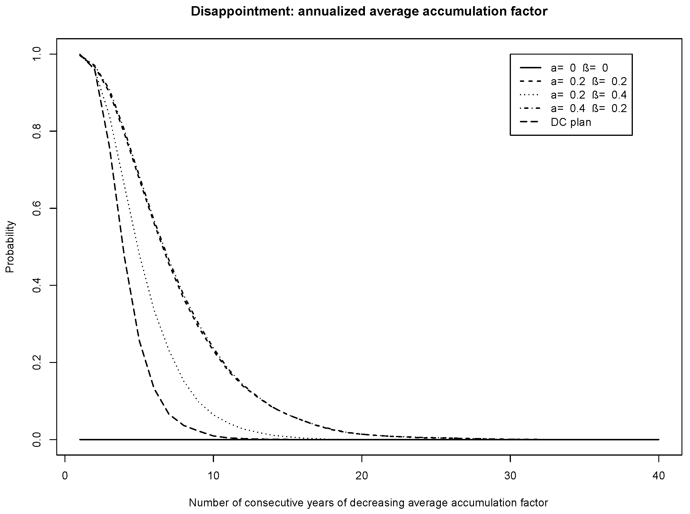
Figure 7 and Figure 8 show the probability of disappointment for the plans, i.e., the probability of a fixed number of years of declining average AAF, for a target funding levels of 100% and 120%, respectively. Members of the plans with the higher target funding level $\overline{F}=120$% (Figure 8) are less likely to suffer disappointment. Thus the higher target funding level gives more security to the members. In all figures, it is observed that members of the risk-sharing plans are more likely to suffer declining average AAFs than DC plan participants. Therefore, communication of this possibility to members is essential for risk-sharing plans.

Figure 9 and Figure 10 show the probability of disappointment for the plans, but for the AAF instead of the average of the AAFs. The message is the same, albeit the disappointment measure is very close to that of the DC plan. Disappointment is reduced by increasing the target funding level. This suggests that members who are easily disappointed should be in a plan with a higher target funding level.

4. Conclusions

The risk-sharing plan presented enables its members to receive more stable increases on their contributions than under a DC plan. However, the downside is that members may face year-on-year reductions in the accumulated value of their contributions, which I call disappointment. There is a higher chance of this than under a DC plan, for the chosen financial market model and membership profile. The possibility of members’ accumulated contributions declining over time would need to be well-communicated to them. However, as the average accumulation factors on the contributions made in the risk-sharing plan are more stable than under a DC plan, a risk-sharing plan may allow members to plan better for their retirement since they have more certainty about the amount of their retirement benefit.

The chance of year-on-year reductions in the accumulated value of contributions can be reduced by increasing the target funding level. This suggests that members who wish to reduce the chance of reductions should be in a plan with a higher target funding level. However, increasing the target funding level means that earlier generations pay for a cushion of assets from which they may not benefit. Instead, the later retiring generations are more likely to benefit from the cushion, in the form of higher accumulation factors granted on their contributions.

The choice of the plan parameters—which determine by how much to adjust the investment strategy, the accumulation factors and the target funding level—are critical to the sustainability of the plan, and the degree of risk-sharing between generations. Based on the studied plans, I draw the following conclusions. The accumulation factor granted on contributions is most sensitive to the parameter that adjusts the investment strategy. The chance of the plan running out of money is most sensitive to the parameter that adjusts the accumulation factors. The target funding level can be used to shift the level of accumulation factors between generations; a higher target funding level means that earlier generations are granted lower accumulation factors than later generations, and vice versa.

The choice of the plan parameters requires a careful study of the expected membership profile, allowing for a financial market model or models. A preliminary analysis by the author, using the membership profiles analyzed in the paper, suggests that the conclusions continue to hold when the financial model is changed. While this paper analyzes a selection of the plan parameters, any implementation in practice would require further analysis to choose appropriate values for the expected plan membership.