
Valuation of Non-Life Liabilities from Claims Triangles


Department of Mathematics, Stockholm University, SE-106 91 Stockholm, Sweden
*
Author to whom correspondence should be addressed.
Risks 2017, 5(3), 39; https://doi.org/10.3390/risks5030039
Submission received: 28 June 2017
/
Revised: 15 July 2017
/
Accepted: 17 July 2017
/
Published: 19 July 2017
Abstract
:This paper provides a complete program for the valuation of aggregate non-life insurance liability cash flows based on claims triangle data. The valuation is fully consistent with the principle of valuation by considering the costs associated with a transfer of the liability to a so-called reference undertaking subject to capital requirements throughout the runoff of the liability cash flow. The valuation program includes complete details on parameter estimation, bias correction and conservative estimation of the value of the liability under partial information. The latter is based on a new approach to the estimation of mean squared error of claims reserve prediction.
1. Introduction
The purpose of the present paper is to describe how the cost-of-capital approach from Engsner et al. (2017), which builds on the approach to market-consistent liability valuation from Möhr (2011), may be implemented using non-life claims triangle data covering both premium and reserve risk. In Engsner et al. (2017), general formulas for cost-of-capital valuation of liability cash flows are provided. For this to become practically relevant in a non-life insurance context, we need to define cash flow dynamics that are consistent with those seen in actual non-life insurance applications.
The undoubtedly most common claims triangle reserving method used in practice is the (distribution-free) chain-ladder method defined in Mack (1993a). This is a pure reserving method, and there is from that perspective no need to define how the model is initiated, since reserving amounts to estimating outstanding costs for already incurred claims. This is in contrast to premium risk, where there is a need to describe how not yet incurred claims will generate future payments. Further, the pan-European insurance regulation Solvency II is constructed to measure, amongst other things, non-life insurance risk expressed in terms of premium and reserve risk. Concerning reserve risk, the Solvency II regulation’s so-called standard formula is based on a one-year re-reserving risk based on a time series version of the classical chain-ladder method; see Merz and Wüthrich (2008). Regarding premium risk, there is no single standard method; for more on this, see, e.g., Gisler (2009); Ohlsson and Lauzeningks (2009). One can here note that these methods do not necessarily have a one-to-one correspondence with the assumptions underlying, e.g., the standard chain-ladder method. We can also remark that there are connections between the consistent multi-period valuation approach from Engsner et al. (2017) and the simplified inconsistent multi-period valuation approach provided by EIOPA; see the definition of the so-called “risk margin” in (European Commission 2015, Article 37).
Moreover, the valuation formulas from Engsner et al. (2017) are based on the payment process dynamics and the resulting capital costs from repeated capital requirements. In practice, we need to define a specific model, estimate parameters and assess both process and estimation uncertainty. Further, in Engsner et al. (2017), it is shown that the general cost-of-capital valuation formulas become analytically tractable when the underlying class of models describing the payment dynamics are Gaussian. Due to this, we give two examples of Gaussian time series payment process models. These claims’ payment generating processes will, in turn, induce natural predictors for outstanding costs stemming from incurred, as well as not incurred claims. The Gaussian models introduced in Section 4 are merely two examples of reasonable models, which in many aspects are similar to the standard chain-ladder method, but which allow for premium risk calculations. For more on time series versions of the chain-ladder method, see, e.g., Buchwalder et al. (2006); Kremer (1984) and (Wüthrich and Merz 2008, chp. 3) and the references therein. Furthermore, for the models introduced in Section 4, we derive parameter estimators using conditional weighted least squares and show that the natural predictors for outstanding payments using plug-in estimation are unbiased. Since the valuation formulas are non-linear functions of the model parameters, plug-in estimators of liability values will be biased. As a consequence of this, we derive an approximate plug-in bias correction for the valuation formulas, and based on that, we approximate the parameter uncertainty using a type of resampled pseudo estimator; see Section 3. These pseudo estimators share many features with the approach to approximate prediction uncertainty in Mack (1993a) and Buchwalder et al. (2006). One can also note that the Gaussian payment processes introduced in Section 4 will induce claims reserving methods. By using the idea of resampled pseudo estimators, we may calculate a type of mean squared error of prediction (MSEP) for the induced reserve estimators, which are consistent with the plug-in bias correction for the valuation formula. In fact, in Lindholm et al. (2017), it is shown that the idea of using resampled pseudo estimators may be used to retrieve the standard MSEP approximation for the chain-ladder method derived in Mack (1993a).
Examples of papers relating to risk-margin-like calculations, apart from the ones mentioned above, are Salzmann and Wüthrich (2010), Wüthrich et al. (2011) and Ferriero (2016). It is demonstrated in Salzmann and Wüthrich (2010) and commented on in Wüthrich et al. (2011) that a cost-of-capital approach to risk-margin calculations leads to evaluations of path-dependent multi-period risk measures that in most cases can neither analytically, nor numerically be calculated. Various proxies are presented in Salzmann and Wüthrich (2010). In Wüthrich et al. (2011), an alternative, computationally more attractive risk margin is defined as the difference between a risk-adjusted reserve and a classical reserve and analyzed using probability-distortion techniques and a Bayesian chain-ladder method. In Ferriero (2016), reserve losses are modeled directly using a stochastic process designed to replicate actuary behavior in repeated re-estimation of reserves. An approximation is made in Ferriero (2016) that allows the risk margin to be approximated without having to solve a backward recursion. In the current paper, we define the risk margin using the multi-period cost-of-capital approach presented in Engsner et al. (2017), in line with how it is defined in Möhr (2011) and Salzmann and Wüthrich (2010). However, by assuming that aggregate paid amounts for different accident and development periods have Gaussian joint distributions, we are in the exceptional situation where the risk margin can be calculated analytically as a solution to a backward recursion. As with any model assumptions, the extent to which specific claims triangle data are consistent with Gaussian model assumptions should be assessed. See Section 5 for further details. In situations where it is likely that aggregate paid amounts are essentially due to a few large claims, Gaussian model assumptions are not suitable.
To conclude, we provide a detailed procedure for how to carry out a consistent multi-period cost-of-capital liability valuation based on claims triangles. This is done for two Gaussian cash flow models including parameter estimators, assessment of parameter uncertainty and a full description of the underlying claims reserving method, which is implied by the cash flow model.
The paper is organized as follows: general results on cost-of-capital valuation for Gaussian cash flows are given in Section 2, which is followed by Section 3, where necessary results on estimation and methods to deal with parameter uncertainty are described. In Section 4, two specific Gaussian cash flow models are introduced and analyzed in detail, and we conclude with a short section on model evaluation (see Section 5), together with numerical illustrations (see Section 6). In order to make the exposition more comprehensive, all proofs are collected in the Appendix.
2. Valuation of Non-Life Insurance Cash Flows
In order to present our approach to the valuation of non-life insurance liabilities, we first need to define the liability cash flows as stochastic processes of a certain kind. We take a rolling one-year risk-free bond as the basis for the numéraire process with value one at the current time. In what follows, unless stated otherwise, all future cash flows are discounted by this numéraire or, equivalently, denoted in units of the numéraire process. Similarly, using historic one-year discount factors from data on one-year risk-free bonds, we may adjust historic cash flow data to be expressed in units of the numéraire process. This data adjustment implies that predictions based on historic payment data are predictions adjusted for the time-value of money. Other choices of traded numéraire processes are possible.
Consider K lines of business providing one-year insurance products: the buyer of the insurance product is not entitled to economic compensation for accidents later than twelve months from the time the product is purchased. For , let denote the incremental claims payment during development year , and let denote the cumulative payments during development years from accidents during accident year , where . For , let:
denote the data from business line k that are known at time t. Calendar year corresponds to the current time. Such a dataset is commonly referred to as a claims triangle, although claims trapezium may be more appropriate. Notice that accident years are fully developed. Notice also that accidents during accident year have not yet occurred. Including accident year in the setup allows for so-called premium risk. Omitting accident year implies that only so-called reserve risk can be studied in the setup. Let:
where we set:
The overall aim is to assign a value to the future liability cash flow from both active contracts (non-incurred claims) and claims from contracts that may still generate claims (incurred, but not reported and reported, but not settled claims). Set and:
Notice that corresponds to non-incurred claims from still active contracts. Further, note that corresponds to the payments during a specific year for all accident years simultaneously, i.e., corresponds to a diagonal in an incremental claims payment triangle. Furthermore, set:
For each k, if accident year is omitted, then is the classical claims reserve. If accident year is included, then the setting allows for analysis of both so-called reserve risk and premium risk.
Let and denote the column vectors with components and , respectively. The value of the liability cash flow will be defined as the value of a static replicating portfolio and the value of a position in the numéraire (one-year bond) needed to handle the residual liability cash flow from imperfect replication by the static replicating portfolio. In general, the choice of replicating portfolio depends on whether the liability cash flow depends on values or cash flows from traded financial assets. For the liability cash flows considered here, we assume that there are no clear dependencies on financial asset values. We choose the replicating portfolio as the one generating the deterministic cash flow . This cash flow is obtained by, for each , buying units of the numéraire (one-year bonds that are rolled forward) at Time 0 and then selling them at time t. The market price of the static replicating portfolio is:
Let be the residual cash flow from imperfect replication. Given a risk-based regulatory framework, such as the one currently in place, the residual cash flow X will give rise to capital requirements. From the costs associated with meeting these capital requirements, a value at Time 0 will be assigned to X. The basis for determining is to consider a hypothetical transfer of the liability cash flow and the replicating portfolio to a separate entity, a so-called reference undertaking, whose sole purpose is the handle the runoff of the liability cash flow. The procedure for determining is as follows.
Let be the value of the residual cash flow from time to time T as seen from Time 0. In particular, since there is no cash flow beyond time T. At time t, the reference undertaking is required to hold the solvency capital , where is the conditional monetary risk measure value-at-risk or expected shortfall , conditional on . Conditioning on means that we only consider information from payment data. The reason for this choice is that we aim for a non-life valuation method that can be easily applied by anyone having access to yearly aggregated claims payment triangle data.
At time t, the reference undertaking has capital that equals the value of the residual cash flow and asks a capital provider, with limited liability, to provide the capital ensuring solvency at time t. Upon providing the capital at time t, the capital provider receives any surplus at time . However, capital is only provided if the expected return is good enough, if:
The value is defined as the value for which capital is provided, but such that capital providers do not obtain better-than-required expected returns. That is, the inequality above is replaced by an equality. In general, is -measurable. Here, in order to derive closed-form valuation formulas, we assume that is -measurable. That is, we assume that future requirements on the expected return on capital from capital providers are known at present time.
From Propositions 1 and 4 and Remark 5 in Engsner et al. (2017), it follows that:
where ○ denotes composition and:
With denoting the space of -measurable random variables Y with , is a mapping satisfying:
properties that are inherited from the risk measure .
Notice that and are conceptually-consistent alternatives to the ill-defined Solvency II quantities risk margin (see (European Commission 2015, Article 37)) and technical provisions, respectively. Thus, corresponds to the Solvency II best estimate (BE). We want to emphasize that the Solvency II risk margin is not properly defined mathematically. For further details, see, e.g., p. 316 in Möhr (2011).
Notice that the definition of the value of the liability cash flow is intimately connected to the particular choice of static replicating portfolio considered here. The procedure for determining is independent of the choice of replicating portfolio, although the value of depends on the replicating portfolio via the residual cash flow X.
In general, no explicit expression can be derived for . However, one important exception is when all cash flows are jointly Gaussian and the cost-of-capital rates are -measurable.
Proposition 1.
Assume that the joint distribution of the random variables:
is Gaussian and, for all t, is -measurable. Then:
where:
with:
where and are defined in Remark 1.
The proof is given in the Appendix.
Notice that Equation (5) makes sense due to the Gaussian model assumption: is a constant and therefore measurable with respect to the trivial -field, which is a subset of .
Remark 1.
The choices and correspond to choices made in the Solvency II regulation, whereas correspond to the Swiss Solvency Test. For an -measurable (discounted) value Z, the conditional monetary risk measures and are defined in terms of the conditional distribution function and quantile function as:
Remark 2.
From the variance decomposition formula,
With and since is independent of under the Gaussian model assumption,
Hence, Equation (4) can be expressed as:
If we have a Gaussian model for the cash flow , then its value is determined by Equation (5) and can be estimated based on suitable estimates of the mean vector and covariance matrix of .
However, the typical situations for the valuation of an aggregate cash flow are models, or at least reserving methods, for the cash flows , . The dependence between the cash flows for different business lines is not well-understood, and independence is often assumed.
Proposition 2.
Suppose the assumptions of Proposition 1 hold and, for , that . Then:
where:
In particular, if for all t, then .
The proof of Proposition 2 is given in the Appendix.
The natural application of Proposition 2 is conservative estimation of the value of the residual liability cash flow in the case of only partial information. Conservative estimates of the conditional variances may be given by the estimates of conditional mean-squared errors of predictions (MSEPs):
Estimation of MSEP is discussed in detail in later sections. The correlations cannot be reliably estimated based on claims triangle data. Proposition 2 provides a flexible tool for assessing the effect of dependence between claims triangles in terms of exogenously-given correlations in line with standard formulas found in regulatory frameworks.
3. Estimation and Parameter Uncertainty
Up to this point, we have discussed liability valuation given general Gaussian cash flow models when all, unspecified, model parameters are fully known. In practice, we will use a specific Gaussian cash flow model to value a certain liability. For this particular model, we will need to estimate an unknown parameter vector . Based on the estimator , a natural estimator of the liability value according to Proposition 1 is the plug-in estimator . However, the estimator is typically biased, since it in general is a non-linear function in terms of the components of , even though individual parameter estimators may be unbiased. Hence, there is in general a need for a bias correction of .
In this section, we will present parameter estimation, estimation of the bias of and, finally, estimation of mean squared error of reserve prediction allowing for conservative estimation of under partial information.
3.1. Parameter Estimation
Here, we present the estimation of model parameters based on the information, , available at Time 0. The Gaussian cash flow models, which will be defined in Section 4, will all be such that the cash flows of different accident years are independent, and for a fixed accident year, the cash flows, incremental or cumulative, are given by dynamic linear regression (autoregressive) models. In common for these models is that it is possible to represent them as a sequence of conditional general linear models, where the sequence runs over development years. That is, the state of our conditional payment process in development year j for all relevant accident years i for the k-th line of business, denoted , conditional on the information available up to satisfying:
By “relevant accident years”, we mean that only payments from accident years i such that is -measurable appear in . Here, denotes a matrix containing relevant (functions of) ’s with ; is the parameter vector of regression coefficients for the j-th conditional linear model; and is multivariate Gaussian with zero mean and covariance matrix , where is some known (deterministic) weight matrix. Moreover, the ’s are independent across indices j and k. The independence w.r.t. k is due to all model parameters being estimated separately for each line of business k, hence neglecting any potential dependencies between lines of business. Further, notice that is defined in terms of vectors , which in the linear model context here are treated as covariates.
From general theory on linear models, we know that the weighted least squares estimator of is given by:
As for standard general linear models, Equation (7) does not provide an estimator for . A natural estimator of is:
where n corresponds to the degrees of freedom and is independent of . We will throughout use an unbiased estimator of . For ease of exposition, we collect all parameters for the model for the k-th line of business in , and we consequently have that:
Regarding the estimation uncertainty, we know from standard theory on general linear models and weighted least squares estimation that:
see, e.g., (Fahrmeir et al. 2013, p. 181). Moreover, using that is a quadratic form of a multivariate Gaussian vector together with standard matrix algebra gives:
The above together with the fact that and are independent fully specifies . Moreover, for ,
which together with:
imply that:
This is a property that will be used below.
Remark 3.
Note that the variance estimator above is unbiased. In practice, making it unbiased corresponds to disregarding some observed data. In a claims triangle setup, data are typically scarce from the beginning, which makes it worth considering the tradeoff between bias and the lack of data.
Remark 4.
Above, we have exploited the fact that the time series models defining the cash flows may be represented as a sequence of conditional general linear models and used conditional weighted least squares estimation. For more on the relation between weighted least squares estimation and maximum likelihood estimation for general linear models, see, e.g., (Fahrmeir et al. 2013, chp. 4.1.2 and chp. 5.1.2). For more on estimation procedures based on both conditional, as well as unconditional approaches for ARMA models, see, e.g., (Christensen 1991, chp. V.5) and (Brockwell and Davis 1987, chp. 8).
3.2. Bias and MSEP
Given the -measurable parameter estimator , the plug-in estimator of is . Notice that is a -measurable function of the -measurable estimator , but for bias correction, we are only interested in correcting for the estimation uncertainty, not the fact that we, e.g., have observed a particular amount of realized payments, which will form the basis for the prediction of future outstanding payments. Notice also that the bias of ,
is zero if one uses a naive plug-in estimator and therefore useless; see Mack (1993a).
In order to obtain a relevant estimator of the bias of , we propose a method that has similarities with the methods in Buchwalder et al. (2006) and Mack (1993a). We introduce a random vector representing parameter uncertainty, which can be regarded as a pseudo estimator. We require that, conditional on past payments, is independent of future payments. Formally,
Moreover, the conditional mean and covariance:
are assumed to exist finitely and will be chosen to reflect estimation uncertainty in sequential estimation of . In the present paper, we will use based on (conditional) weighted least squares; see Section 3.1 and further details in Section 4. Based on the calculations in Section 3.1 concerning the properties of the estimator , we require that is chosen such that are independent,
Notice that is block diagonal with blocks that are again, due to Equation (11), block diagonal with blocks . Thus, we have fully specified and .
Remark 5.
Note that the definition of shares many features with, e.g., Buchwalder et al. (2006), as well as England and Verrall (1999).
Remark 6.
Note that trivially, it holds that for :
that is, the sub-matrices defining are not chosen w.r.t. arbitrary conditionings on ’s.
Using the pseudo estimator , we define the bias, conditional on , of with respect to plug-in parameter uncertainty as:
Now, let and:
which gives:
The bias of as an estimator of is due to the ’s being nonlinear functions of the components of its vector-valued argument. The requirement is easily met in the dynamic linear-regression-type models we will consider. What remains is to quantify such that it leads to accurate estimation of the bias of . The bias is approximated by approximating by its second degree Taylor expansion:
where denotes the Hessian of . Some matrix algebra yields the following proposition:
Proposition 3.
Remark 7.
Notice that in Proposition 3 is a -measurable function of θ. We suggest plug-in estimation of with plug-in in place of θ. The resulting quantity is then used to correct the estimate of the liability value from Proposition 1. Further, notice that if , then the estimator of simplifies to:
We now turn to the estimation of MSEP. The natural plug-in estimator of outstanding claims costs is given by . Following the definition in Mack (1993a), the mean squared error of prediction (MSEP) for the claims reserve for the k-th line of business is given by:
which may be re-written as:
As in Mack (1993a) and Buchwalder et al. (2006), the first term in the MSEP expression corresponds to the “process variance”, which may be approximated using a plug-in estimator. The second term, corresponding to parameter uncertainty or “estimation error”, will collapse to zero if a plug-in estimation is used. Considerable effort has been made on how to estimate the parameter uncertainty; see, e.g., Mack (1993a) and Buchwalder et al. (2006) and the references therein, which rely on various ways to condition on data. In the present paper, we will adopt the procedure described for the bias correction in Proposition 3 in order to ascertain consistency between the approximations. Based on the above argumentation, we introduce the following MSEP:
which is close to (Buchwalder et al. 2006, Approach 3) and Mack (1993a). The equality between Equations (15) and (16) is assured by Equation (12).
Moreover, if we assume that the plug-in estimator is an unbiased estimator of the claims reserve, the following approximation to MSEP* is obtained by repeating the steps of Proposition 3:
In Lindholm et al. (2017), these relationships are explored in more detail with respect to the results of Buchwalder et al. (2006) and Mack (1993a). More specifically, it is shown that Equation (17) using plug-in estimation coincides with the standard MSEP calculation for the chain-ladder method given in Mack (1993a).
Remark 8.
Note that Proposition 2 may be approximated using MSEP* as an approximation of the variances needed in the specification of the quantity A, which also captures estimation error.
4. Gaussian Cash Flow Models
In the present section, we will describe two different Gaussian cash flow models and their parameter and reserve estimators. Further, the effect of estimation uncertainty is analyzed, and in particular, we derive bias corrections for the cost-of-capital valuation using plug-in estimators and calculate the approximate mean squared errors of prediction for expected future costs. For more on time-series-reserving methods, see, e.g., Buchwalder et al. (2006); Kremer (1984); Merz and Wüthrich (2008). One can also note that, e.g., Buchwalder et al. (2006) provide a time-series model with Gaussian errors, which does not yield a Gaussian process. In the present paper, we need the entire cash flow model to be Gaussian for the valuation formulas from Section 2 to be applicable, thus disqualifying the model from Buchwalder et al. (2006).
4.1. An Autoregressive Model for Incremental Amounts
Let denote the premium volume for accident year i (or a similar exposure measure). It is assumed that all are known constants. Let denote the normalized incremental claims payments.
We assume the following stochastic model for incremental claims payments:
where and for every k, the , , are mutually independent and standard normally distributed.
The incremental Gaussian cash flow model defined by Equation (18) implies the following basic properties:
Proposition 4.
The proof is presented in the Appendix.
Note that Proposition 4 contains all information needed in order to be able to value a liability following the dynamics described by Equation (18) when all parameters are assumed to be known. In practice, we need to estimate the parameters and in order to be able to use the valuation formulas. Given parameter estimates, the valuation formulas are then evaluated based on plug-in estimates. Further, from Proposition 4, we see that the natural plug-in reserve estimator:
is unbiased given that and are unbiased and that and are uncorrelated for . Proposition 6 below affirms that this indeed is the case.
Moreover, since is a non-linear function in terms of , the liability valuation formula using plug-in estimates will not be unbiased. Below, we will present an approximate bias correction for the valuation formula based on the incremental Gaussian cash flow model from Equation (18).
Remark 9.
As commented upon above, the valuation formula is a non-linear function in terms of model parameters. In order for the natural reserve estimator to be unbiased, it is necessary that the and are unbiased. Due to the valuation formula’s non-linearity, it is, however, less relevant to require unbiased estimation of the , since the entire valuation formula most likely will need a bias correction regardless of whether the are unbiased or not.
We will now proceed with parameter estimation.
4.1.1. Parameter Estimators and Predictors
As described in Section 3.1 above, the incremental model defined by Equation (18) may be expressed in terms of a sequence of conditional general linear models defined as follows: Let:
compactly as where has zero mean and covariance matrix with , where all are known. Furthermore, recall that this is a model that is conditional on , which is put in , here treated as a set of covariates.
By using the results from Section 3.1 based on the specification above, the parameter estimators for the incremental model may be written out explicitly as follows:
Proposition 5.
The (conditional) weighted least squares estimators for model Equation (18) are given by:
and:
given that and:
where and:
Further, as commented on in Section 3.1, all ’s are unbiased, but it is possible to say more:
Proposition 6.
The estimators , , are unbiased and uncorrelated.
The proof is given in the Appendix and is based on the tower property conditioning on .
In the beginning of Section 4.1, plug-in estimation of outstanding costs was discussed. That is, based on the observed data :
Moreover, we set:
and .
Proposition 7.
for with . Moreover, .
The proof is given in the Appendix.
We may now move on to treat parameter uncertainty with respect to liability valuation and claims reserve (MSEP).
4.1.2. Bias of the Liability Valuation Using Plug-In Estimators
The procedure for approximating the plug-in bias of the valuation formula from Section 3 is fully defined up to the specific parametrization of the model being studied. In the Appendix, the details are presented for the incremental model, and the results for bias correction are given in Proposition 8 below. If we introduce:
we may state the approximate bias correction as follows:
Proposition 8.
The plug-in estimation bias for the incremental Gaussian model defined by Equation (18) is approximated by:
where:
and:
As discussed above, the plug-in estimation bias from Proposition 8 is again a function in terms of the unknown model parameters and is estimated using .
The proof of Proposition 8 is given in the Appendix.
4.1.3. Mean Squared Error of Prediction
As pointed out in Section 3.2, it is shown in Lindholm et al. (2017) that the proposed MSEP calculation given by Equation (17) for the classical claims reserve, that is when not considering premium risk, will coincide with that of Mack (1993a) for the chain-ladder method. Due to the dependence between and , these calculations turn out to be very complicated. We will now provide explicit formulas for the classical claims reserve for a single line of business, but leaving out the explicit dependence on a particular line of business “k”. This is in accordance with the situation in Mack (1993a). Further, due to the complexity of the calculations, we only provide explicit formulas for the MSEP (= ) when all :
Proposition 9.
The MSEP for the classical claims reserve for the autoregressive incremental model given by Equation (18) with , may be approximated according to:
where:
and:
where:
The proof follows the steps of Mack (1993a) closely and is given in the Appendix.
Remark 10.
The proof of Proposition 9 in the case when turns out to be very tedious following Mack (1993a). It is however possible to calculate the approximate MSEP following Equation (17), but not very informative. For the case , Lindholm et al. (2017) shows that the results coincide with those of Mack (1993a).
Remark 11.
Above, we provide formulas for the classical claims reserve. If we want to include premium risk, as well, this is straightforward to do using Equation (17) when including accident year . In theAppendix, is given in the derivation of Proposition 8, and is easily calculated, since it is multilinear in terms of the components of θ. We do not write out these calculations explicitly, due to these becoming even more involved than the expressions above, and do not provide any further insights.
4.2. An Autoregressive Model for Cumulative Amounts
We assume the following model for cumulative claims payments :
where, for every k, the , , are mutually independent and standard normally distributed. This model is consistent with the chain-ladder prediction method, with a structure for the conditional variances that ensures that all incremental and cumulative payments are jointly Gaussian.
Remark 12.
Note that the actual reserve estimator based on model Equation (20) will not coincide with that of the standard chain-;adder method; see further Section 4.2.1. Further, note that for the standard chain-ladder method, there is no need to initiate the data-generating process, i.e., is always observed, but in the present paper, this step is needed in order to capture premium risk.
Remark 13.
The techniques used for the derivation of the basic properties of the cumulative model will be identical to those used in Section 4.1 for the incremental model. Further, for the cumulative model, the actual calculations will be simpler than for the incremental model, and due to this, most calculations in this section will be kept very brief.
Proposition 10.
The proof is given in the Appendix.
One can here note that for the classical claims reserve, i.e., when omitting year , it holds that:
which suggests the following natural reserve estimator:
4.2.1. Parameter Estimators and Predictors
In order to be able to use the valuation formulas, we need to obtain parameter estimators. Following Section 4.1.1, making the obvious changes to arrive at a sequence of (conditional) general linear models describing model Equation (20), we get the following proposition:
Proposition 11.
The (conditional) weighted least squares estimators of the parameters , from model Equation (20), are given by:
and:
given that . Further, and all and are uncorrelated, and and all and are unbiased.
The proof of Proposition 11 follows the corresponding proofs for the incremental model verbatim.
4.2.2. Bias of the Liability Valuation Using Plug-In Estimators
By repeating the same steps as for the incremental model, it is possible to arrive at the following approximation of the plug-in estimation bias from Proposition 8:
Proposition 12.
The plug-in estimation bias for the cumulative Gaussian model defined by Equation (20) is approximated by:
where:
and:
As before, the plug-in estimation bias from Proposition 12 is again a function in terms of the unknown model parameters and is estimated using .
4.2.3. Mean Squared Error of Prediction
In relation to the approach in Mack (1993a) for approximating the classical claims reserve MSEP, it is perhaps not surprising that the cumulative model from Equation (20) will prove easier to treat than the incremental model. Again, we will focus on the situation in Mack (1993a), that is a single line of business (without explicit reference to line of business “k”) and no premium risk included (accident year is omitted). The following approximation of MSEP (=) for the cumulative payment model is obtained by directly applying the methods of Mack (1993a):
Proposition 13.
The MSEP for the autoregressive cumulative model given by Equation (20) may be approximated according to:
where:
The proof of Proposition 13 is identical with that of Theorem 3 and the Corollary to Theorem 3 in Mack (1993a), given the parameter estimators for model Equation (20). This is a consequence of the underlying model structure being consistent with that of the standard chain-ladder method. The proof is hence omitted, but the steps follow those of the proof of Proposition 9.
Again, as described in Remark 11, it is straightforward to calculate the MSEP for the expected future costs, including premium risk, but these calculations are omitted.
5. Some Comments on Model Validation: In-Sample and Out-Of-Sample Performance
The focus of the present paper is to describe how to carry out a fully-data-driven cost-of-capital valuation based on claims triangles. Above, we have introduced two Gaussian models for which explicit calculations are possible including estimation and treating parameter uncertainty. Due to that, we have introduced two different models with different (maximal) numbers of parameters; there is a need to assess both the in-sample and the out-of-sample performance of the models.
As commented upon above, both models may be treated as a series of Gaussian linear models. Thus, it is recommended to carry out standard statistical residual analysis and tests of model assumptions for linear models. A detailed description on how this analysis may be implemented for the chain-ladder method is described in Mack (1993b); see also (Wüthrich and Merz 2008, chp. 11).
Further, regarding model selection, including significance tests for parameters, one can note that the two model classes are nested in the classical sense, which means that it is possible to carry out standard likelihood ratio tests (LRT), but other metrics such as AIC/BIC may be considered. Due to that, the models studied in the present paper are Gaussian, and there are no difficulties in determining (conditional) likelihoods. Given this, it is possible to analyze, e.g., LRT and AIC/BIC.
Moreover, since the models’ actual purpose is to be used for out-of-sample prediction, it is reasonable to try to assess the out-of-sample performance. A straight forward out-of-sample performance is to exclude one or two observed diagonals and analyze the corresponding out-of-sample prediction performance. In general, it often is not recommended to exclude more than one or two years of data due to the lack of representative yearly data.
6. Numerical Example
In this section, we illustrate the incremental model in Equation (18) and the cumulative model in Equation (20) and demonstrate the implementation of the results in this paper.
Recall from Section 2 that the models and methods presented assume that historical data and future cash flows are adjusted for the time value of money. The aim of the numerical example in this section is simply to clarify and demonstrate the use of the framework presented earlier. In order to keep the numerical example brief and focus on methodological aspects, we ignore discounting and preprocessing of historical data here.
The data we use are the run-off triangle from Table 1 in Mack (1993a). In order to be able to use the unbiased estimators of the , we remove the last two columns of this triangle. We could use maximum likelihood estimation or some form of extrapolation of the , but the purpose here is not to compare methods for estimating the tail variances; we thus simply remove the last two columns. The data are fairly similar between accident years, and for illustrative purposes, it should suffice to set the weights equal to one for all accident years.
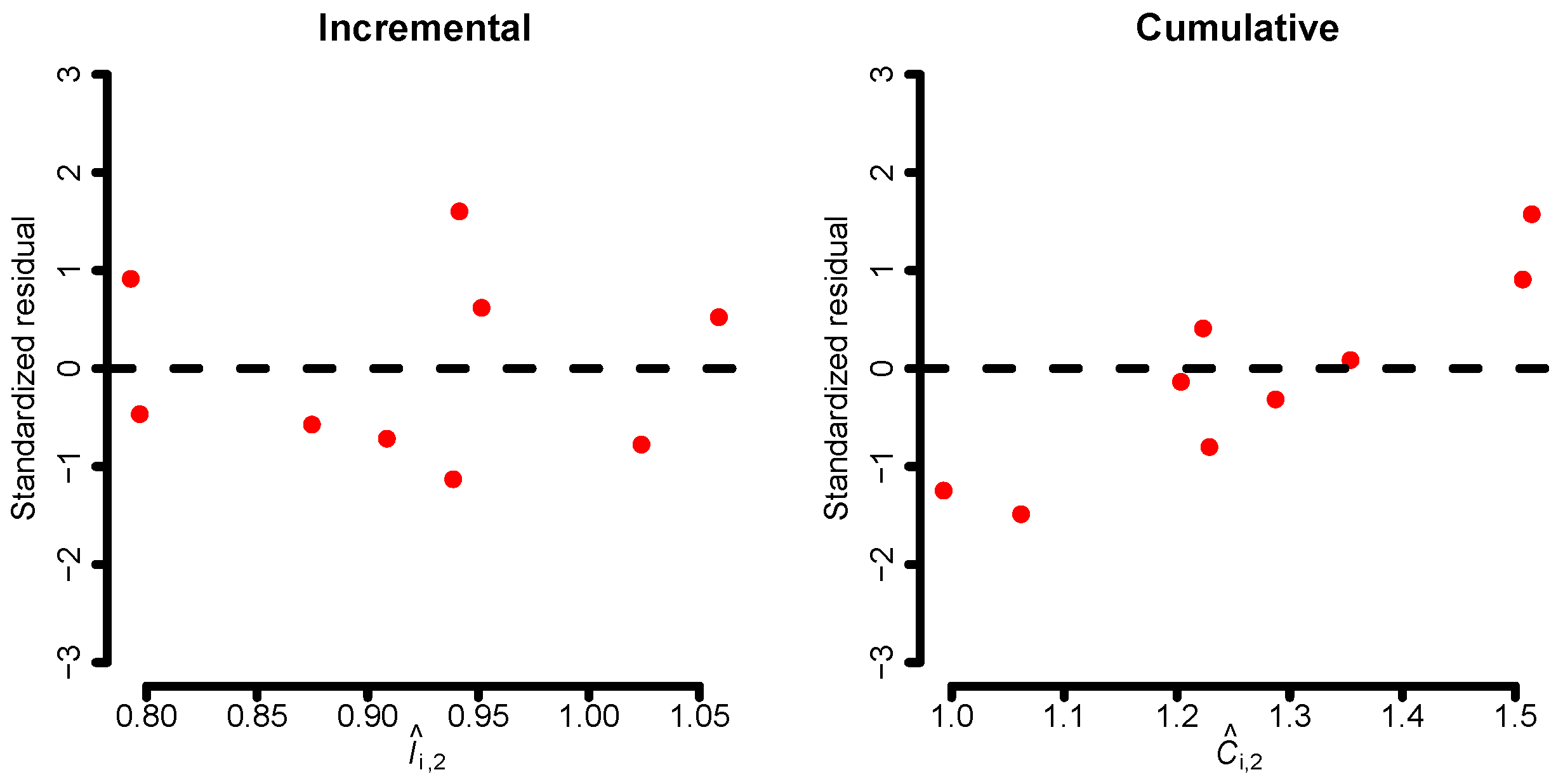
If we fit the incremental and cumulative models to the data, it is recommended to analyze standardized residuals and linearity for each development year and model. This is illustrated in Figure 1, where the standardized residuals for the second development year are shown for both models. There, we see that the residuals of the cumulative model have a systematic pattern implying that the cumulative linear structure defined by the model in Equation (20) does not capture the dynamics of the data well. This is an artifact of the lack of an intercept. However, the small sample size hinders us from making any definitive claims.
Before we proceed with calculating the cost-of-capital margin, etc., we make a brief assessment of the model performance given ideal circumstances. This is done by fitting the incremental and cumulative models to the data, considering these fits as the true models. Given the fitted parameters, we then simulate complete rectangles of data on which we re-fit the two models and plot . The result of this can be seen in Figure 2. Both models seem to be performing similarly regardless of which model is simulated.
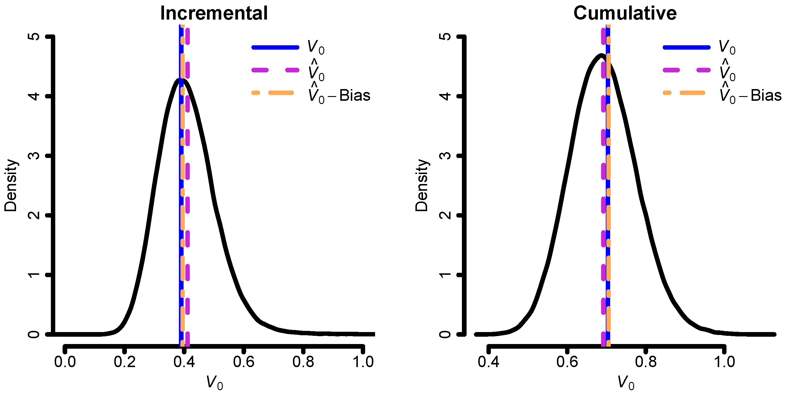
With the aim of illustrating the bias correction of the cost-of-capital margin, we next simulate new triangles from the “true” models and fit the correctly specified model to each. That is, the incremental model is fitted to data simulated from the incremental model, and the cumulative model is fitted to data simulated from the cumulative model. Then, we estimate the cost-of-capital margin (see Equation (5)) and its bias correction for each simulated triangle using the cost-of-capital rate , which is in alignment with the current Solvency II directive. This can then be compared to the true cost-of-capital margin, which we assume known since we consider the models fitted to the original data to be the true models. The results can be seen in Figure 3. The bias correction does seem to work quite well. It should be noted that the expectation part of the liability value , i.e., the best estimate (BE), in the current example is much larger than the cost-of-capital margin. Thus, the bias correction will, in this situation, have a small impact on the estimated liability value; see Table 1.
Proposition 2 provides an upper bound on , denoted ; see Equation (6). Moreover, as commented on in Section 2, the cost-of-capital margin is related to the Solvency II Risk-Margin (RM). In (EIOPA 2015, Guideline 61), the following approximation of RM is suggested:
where in our setting. The Solvency II regulation provides one-year non-life insurance risk standard deviations in the range of 10–20%, depending on the line of business, which form the basis for the SCRcalculations. For the dataset from Mack (1993a), it is not clear from which line of business the data stem. Thus, we use:
Note however that the calculations are based on the standard deviations of the one-year claims development results, which are roughly 4% and 8% of the BE for the incremental and cumulative models, respectively. These values should be compared to the ones above, which are in the range of 10–20%. Consequently, we expect and RM to be considerably lower than the corresponding standard formula results. In Table 1, we have summarized , and RM. Furthermore, the table also includes , BE, and RMSEP. Notice that when including premium risk, we cannot calculate the Solvency II RM without making further assumptions on premium volumes. For the part of Table 1 with premium risk, we have set premium volumes consistent with weights equal to one. Furthermore, note that the cost-of-capital margin cannot be calculated for the chain-ladder model, nor can we calculate any quantity involving premium risk since there is no initiation in the first column. The RMSEP for the chain-ladder model is calculated according to Mack (1993a), and is calculated according to Merz and Wüthrich (2008). Hence, it is possible to calculate RM for the chain-ladder model without premium risk. Turning to the results, from Table 1, it is seen that and are of comparable order and that the corresponding RM values are lower than and of a size comparable to . The cumulative model has almost double the cost-of-capital margin compared to the incremental model. This can most likely be explained by the fact that the intercepts in the incremental model catch some of the variation that is put into the variance parameters of the cumulative model. This is also seen in and RMSEP.
Acknowledgments
The authors would like to thank the referees for their comments and suggestions that improved the paper.
Author Contributions
The authors have contributed equally to this paper.
Conflicts of Interest
The authors declare no conflict of interest.
Appendix A. Proofs
Appendix A.1. Proof of Proposition 1
Proof.
The statement follows from minor modifications of the proof of Proposition 6 in Engsner et al. (2017). Here, different values appear instead of a common value . Moreover, since the cash flow of the replicating portfolio is -measurable, . ☐
Appendix A.2. Proof of Proposition 2
Proof.
The relation holds for -fields and a random variable Y with finite variance. For Gaussian models, the conditional variance expressions correspond to variances of conditional distributions of a multivariate Gaussian random vector, where Y is one component, and the -fields correspond to subsets of components. In particular, with , , and , . Hence,
For a given and , solving for the standard convex optimization problem:
yields the unique maximizer and maximum:
Notice that the expression Equation (5) for is of the form with . For these ’s, . ☐
Appendix A.3. Proof of Proposition 4
Proof.
Notice that for ,
where:
It remains to determine the conditional variances. Due to independence between accident years:
Under the assumption for all and all t,
☐
Appendix A.4. Proof of Proposition 6
Proof.
Let:
First, notice that:
Secondly, with , and ,
and similarly for products with more factors. ☐
Appendix A.5. Proof of Proposition 7
Proof.
Since each component of is a linear combination of predictors , the second statement follows immediately from the first statement. ☐
Appendix A.6. Proof of Proposition 8
Proof.
In order to arrive at the conclusion of Proposition 8, we need to specify and calculate and .
Based on the matrix expressions presented in Section 3.1 and Section 3.2, it is straightforward to deduce that:
where we have omitted the notation for corresponding to the line of business. As described in Section 3.2, is obtained by (independent) stacking of . Turning to the calculation of and for the incremental model given by Equation (18), we have:
which immediately gives us that the following components are the only non-zero contributions:
and so:
By combining the above, we arrive at the desired result. ☐
Appendix A.7. Proof of Proposition 9
Proof.
As in the proof of Theorem 3 in Mack (1993a), the process variance is already calculated (see Proposition 4), and consequently, its estimator is again a straightforward plug-in estimator. The complicated part is to take care of the estimation error. First, consider a single accident year i and the natural reserve estimator , which gives us:
Thus, by combining the above, it holds that:
The MSEP for the total reserve R is obtained in the same way as for the individual accident years, but there is a need to treat terms that describe the dependence between two accident years i and , that is:
which follow analogously from the single accident year situation, i.e.,
☐
Appendix A.8. Proof of Proposition 10
Proof.
Notice that from:
it follows that:
from which the conclusion follows. ☐
Appendix A.9. Proof of Proposition 12
Proof.
The steps for the cumulative model will again be identical to those for the incremental model, but simpler. For further details, we refer to Proof Appendix A.6.
To start off, is constructed based on , where:
for . For the cumulative model, we have:
which gives us that the only non-zero elements of and turn out to be:
and consequently:
Given the above, the results of the proposition follows. ☐
References
- Brockwell, Peter J., and Richard A. Davis. 1987. Time Series: Theory and Methods. Springer Series in Statistics; New York: Springer. [Google Scholar]
- Buchwalder, Markus, Hans Bühlmann, Michael Merz, and Mario V. Wüthrich. 2006. The mean square error of prediction in the chain ladder reserving method (Mack and Murphy revisited). Astin Bulletin 36: 521–42. [Google Scholar] [CrossRef]
- Christensen, Ronald. 1991. Linear Models for Multivariate, Time Series, and Spatial Data. Berlin: Springer Science & Business Media. [Google Scholar]
- EIOPA. 2015. Guidlines on the valuation of technical provisions. Official Publication of EIOPA. EIOPA-BoS-14/166 EN. [Google Scholar]
- England, Peter, and Richard Verrall. 1999. Analytic and bootstrap estimates of prediction errors in claims reserving. Insurance: Mathematics and Economics 25: 281–93. [Google Scholar] [CrossRef]
- Engsner, Hampus, Mathias Lindholm, and Filip Lindskog. 2017. Insurance valuation: A computable multi-period cost-of-capital approach. Insurance: Mathematics and Economics 72: 250–64. [Google Scholar]
- European Commission. 2015. Commission Delegated Regulation (EU) 2015/35 of 10 October 2014. Official Journal of the European Union 58. [Google Scholar]
- Fahrmeir, Ludwig, Thomas Kneib, Stefan Lang, and Brian Marx. 2013. Regression: Models, Methods and Applications. Berlin: Springer Science & Business Media. [Google Scholar]
- Ferriero, Alessandro. 2016. Solvency capital estimation, reserving cycle and ultimate risk. Insurance: Mathematics and Economics 68: 162–68. [Google Scholar]
- Gisler, Alois. 2009. The insurance risk in the SST and in Solvency II: Modelling and parameter estimation. SSRN Manuscript. Available online: https://papers.ssrn.com/sol3/papers.cfm?abstract_id=2704364 (accessed on 15 July 2017).
- Kremer, Erhard. 1984. A class of autoregressive models for predicting the final claims amount. Insurance: Mathematics and Economics 3: 111–19. [Google Scholar]
- Lindholm, Mathias, Filip Lindskog, and Felix Wahl. 2017. Comments on the classical chain-ladder MSEP calculation. Unpublished manuscript. Unpublished manuscript. [Google Scholar]
- Mack, Thomas. 1993a. Distribution-free calculation of the standard error of chain ladder reserve estimates. Astin Bulletin 23: 213–25. [Google Scholar] [CrossRef]
- Mack, Thomas. 1993b. Measuring the variability of chain ladder reserve estimates. Casualty Actuarial Society Forum 1: 101–83. [Google Scholar]
- Merz, Michael, and Mario V. Wüthrich. 2008. Modelling the claims development result for solvency purposes. Casualty Actuarial Society E-Forum Fall 2008, 542–68. [Google Scholar]
- Möhr, C. 2011. Market-consistent valuation of insurance liabilities by cost of capital. Astin Bulletin 41: 315–41. [Google Scholar]
- Ohlsson, Esbjörn, and Jan Lauzeningks. 2009. The one-year non-life insurance risk. Insurance: Mathematics and Economics 45: 203–8. [Google Scholar] [CrossRef]
- Salzmann, Robert, and Mario V. Wüthrich. 2010. Cost-of-capital margin for a general insurance liability runoff. Astin Bulletin 40: 415–51. [Google Scholar]
- Wüthrich, Mario V., Paul Embrechts, and Andreas Tsanakas. 2011. Risk margin for a non-life insurance run-off. Statistics & Risk Modeling with Applications in Finance and Insurance 28: 299–317. [Google Scholar]
- Wüthrich, Mario V., and Michael Merz. 2008. Stochastic Claims Reserving Methods in Insurance. Hoboken: John Wiley & Sons, vol. 435. [Google Scholar]
Figure 1.
Standardized residuals for the second development year for the incremental model (left) and for the cumulative model (right). Fitted values are in millions.
Figure 1.
Standardized residuals for the second development year for the incremental model (left) and for the cumulative model (right). Fitted values are in millions.

Figure 2.
Distribution of the prediction error for the incremental and cumulative models when fitted to incremental data (left) and cumulative data (right). Values are in millions.
Figure 2.
Distribution of the prediction error for the incremental and cumulative models when fitted to incremental data (left) and cumulative data (right). Values are in millions.
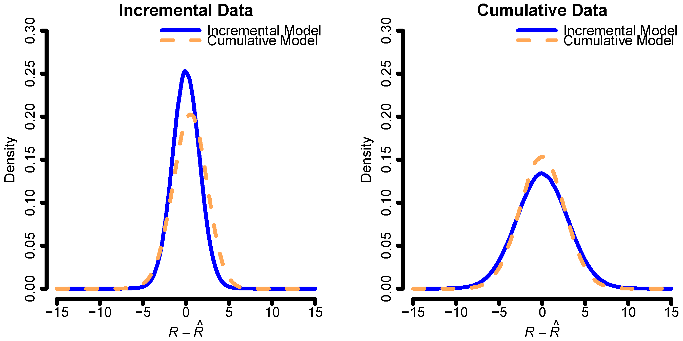
Figure 3.
Distribution of the cost-of-capital margin for the incremental model (left) and the cumulative model (right). Values are in millions.
Figure 3.
Distribution of the cost-of-capital margin for the incremental model (left) and the cumulative model (right). Values are in millions.


Table 1.
Summary table. Values are expressed in millions. RM, risk-margin; BE, best estimate.
| Model | RM | BE | RMSEP | ||||
|---|---|---|---|---|---|---|---|
| With premium risk | |||||||
| I | 0.39 | 0.44 | 0.31 | 18.47 | 18.08 | 1.09 | 1.58 |
| C | 0.70 | 0.87 | 0.83 | 19.94 | 19.24 | 2.12 | 2.67 |
| Without premium risk | |||||||
| I | 0.31 | 0.38 | 0.25 | 13.69 | 13.38 | 0.93 | 1.33 |
| C | 0.51 | 0.67 | 0.54 | 15.03 | 14.52 | 1.64 | 2.06 |
| CL | – | – | 0.71 | – | 14.77 | 1.18 | 1.51 |
© 2017 by the authors. Licensee MDPI, Basel, Switzerland. This article is an open access article distributed under the terms and conditions of the Creative Commons Attribution (CC BY) license (http://creativecommons.org/licenses/by/4.0/).
Share and Cite
MDPI and ACS Style
Lindholm, M.; Lindskog, F.; Wahl, F. Valuation of Non-Life Liabilities from Claims Triangles. Risks 2017, 5, 39. https://doi.org/10.3390/risks5030039
AMA Style
Lindholm M, Lindskog F, Wahl F. Valuation of Non-Life Liabilities from Claims Triangles. Risks. 2017; 5(3):39. https://doi.org/10.3390/risks5030039
Chicago/Turabian StyleLindholm, Mathias, Filip Lindskog, and Felix Wahl. 2017. "Valuation of Non-Life Liabilities from Claims Triangles" Risks 5, no. 3: 39. https://doi.org/10.3390/risks5030039
Note that from the first issue of 2016, this journal uses article numbers instead of page numbers. See further details here.