A Low Price Correction for Improved Volatility Estimation and Forecasting

Abstract

In this work, we focus on volatility estimation which plays a crucial role in risk analysis and management. In order to improve value at risk (VaR) forecasts, we discuss the concept of low price effect and introduce the low price correction which does not require any additional parameters and instead of returns it takes into account the prices of the asset. Judgement on the forecasting quality of the proposed methodology is based on both the relative number of violations and VaR volatility. For illustrative purposes, a real example from the Athens Stock Exchange is fully explored.

1. Introduction

In finance, one of the main goals is the estimation of volatility, since it is crucial in risk analysis and management. When we refer to volatility, we refer to the conditional standard deviation of asset returns. In financial modeling, the view has been consolidated that the asset returns are preferred over prices since they are stationary (Meucci (2009); Shiryaev (1999)). Moreover, the volatility of returns can be successfully forecasted and is essential for risk management (Poon and Granger (2003); Andersen et al. (2001)).

In order to forecast the asset volatility, a number of different models have been developed over the years. Each of them offers an answer to a specific aspect of the problem at hand. The most important approaches in this never ending quest for better estimations are Moving average models (MA), Exponentially weighted moving average models (EWMA), Autoregressive conditional heteroskedasticity models (ARCH), Generalized ARCH (GARCH) models and their extensions, Asymmetric and power GARCH models (APARCH) and Fractionally integrated GARCH models (FIGARCH). For details on the above modelling approaches, see, among others Engle (1982); Bollerslev (1986); Robinson (1991); Baillie et al. (1996); Poon and Granger (2003); Taylor (2004) and Belkhouja and Boutahary (2011).

The need that has driven researchers to introduce and explore such models is the fact that after extensive investigation on the statistical properties of financial returns, three properties have shown to be present in most, if not all, financial returns. Their existence has been the source of most problems associated with the estimation of the underlying risk of assets. These are often called the three stylized facts of financial returns and are Volatility clusters, Fat tails and Nonlinear dependence (Demirgüç-Kunt and Levine (1996); Cont (2001)).

The first property, volatility clusters, relates to the observation that the magnitudes of the volatilities of financial returns tend to cluster together, so that we observe many days of high volatility, followed by many days of low volatility. This, in most cases, is due to some economic news (Cont (2007); Cakan et al. (2015)).

The second property, fat tails (often called heavy-tailed), points to the fact that financial returns occasionally have very large positive or negative returns, which are very unlikely to be observed, if returns were normally distributed (da Cruz and Lind (2012)).

Finally, the non-linear dependence (NLD) of financial returns refers to the observed sharp increases in correlations between assets during financial crises. If returns are linearly dependent, the correlation coefficient describes how they move together. If they are non-linearly dependent, the correlation between different returns depends on the magnitudes of outcomes. For example, it is often observed that correlations are lower in "bull" markets than in “bear” markets, while in a financial crisis they tend to reach 100% (Hsieh (1989); Booth et al. (1994); Cont (2001)).

In recent years, in order to forecast returns and volatility of returns at the same time, new models have been introduced. One very important finding was the existence of the leverage effect (Black (1976); Christie (1982). The leverage effect emerges from the negative correlation which is sometimes observed between stock returns and volatility. The mechanism behind that is the fact that negative news usually increases the volatility of an asset, while good news does the opposite. Returns, on the other hand, act in the exact opposite way.

The increase in complexity of both the financial system and the nature of the financial risk, results in models with limiting reliability. The complexity of the financial risk comes from the fact that although endogenous risk could be disregarded in a typical financial system, this is not true in a financial system in crisis (Danielsson and Shin (2003)). The problem becomes more perplexed since at least one of the above three properties is almost always present. Hence, in extreme economic events, such models become less reliable and in some instances, fully unreliable and consequently produce inaccurate risk measurements. This has a great impact on many financial applications, such as asset allocation and portfolio management in general, derivatives pricing, risk management, economic capital and financial stability (based on Basel III accords).

Because of all the above mentioned issues, more and more complicated models were introduced in order to include these facts. The more complicated the model we use for volatility estimation, the larger the number of parameters that need to be estimated. Hence, more observations will be needed which results in the inclusion of older observations that may not be representative of reality in the analysis.

Assuming that the underlying mechanism of economic phenomena (the same applies to physical or biological phenomena) is quite complex, then any econometric model, no matter how complex or advanced it may be, is still unable to fully capture the entire set of explanatory factors that govern global economy. Consequently, risk models although they are becoming more and more complicated, are not necessarily improving their forecasting ability and most importantly, they will most likely fail at a time of economic crisis. For a related discussion triggered by the US crisis of 2007, see Greenspan (2008). Furthermore, risk models utilize only the returns of an asset while ignoring the prices.

In order to answer all the questions raised above, we discuss the concept of low price effect and recommend a low price correction for improved VaR forecasts which does not require any additional parameters and takes into account the prices of the asset. For judging the forecasting quality of the proposed methodology, we rely on two measures, namely the relative number of violations, known as the violation ratio, and the VaR volatility. For comparative purposes, both measures are evaluated with and without the low price correction.

The paper is organized as follows. The low price effect together with the proposed methodology for improved volatility estimation is presented in detail in Section 2. The basic characteristics of backtesting can be found in Section 2.1. For the implementation, in Section 3, we use the National Bank of Greece stock (of Athens Stock Exchange) which exhibits violent changes in its price, together with volatility structural changes due to the abnormal economic environment under which it operates.

2. Low Price Effect and Low Price Correction

If the price of an asset is extremely low because of extreme economic conditions and the market does not operate with small enough accuracy, then volatility of returns will be automatically increased. This increase which is the result of a minimum possible return that exists for the asset, is often neglected since the estimating process is based solely on returns rather than taking additionally, into consideration, the asset prices.

Definition 1. 

The minimum possible return $mpr$ of an asset is the logarithmic return that the asset will produce if its value changes by the minimum accuracy with which the market operates. Let c be the accuracy under which the market operates and $p_t$ be the asset value at time t. Then, the minimum possible return $mp{r}_t$ at time t is given by:

$$mp{r}_t=log\left(\frac{p_t+c}{p_t}\right)$$

Remark 1. 

Although in most stock exchange markets the accuracy is 0.1 cents (0.001 euros/dollars), Definition 1 allows the use of any positive value for c.

Remark 2. 

Since logarithmic returns are symmetric, the minimum possible return is the same for both upward and downward movements of the asset price.

The low price effect (or low price anomaly) was initially documented by Fritzmeier (1936) who noticed that low-priced stocks were characterized by higher returns but at the same time become more variable. Allison and Heins (1966) and Clenterin (1951) declared that the source of the price risk was not the low price but the low quality of stocks perceived by investors. We proceed below with a slightly different definition of the low price effect which sheds some extra light on the phenomenon.

Definition 2. 

Low price effect (lpe) is the inevitable increase of variance in stocks with low prices due to the existence of a minimum possible return.

This increase in volatility was previously observed, but it was addressed as the aftermath of the increased returns while it appears to be exactly the opposite. The increase in returns is due to the increase in the volatility. In order to make it clear, let us assume that the value of an asset is equal to 0.19€ and the market operates with 0.001€ accuracy. Then, the minimum possible return for the asset is 0.5%. Also, all possible (logarithmic) returns for the asset on this specific day are the integer multiples of the minimum possible return. This will result in the stock movement becoming even more nervous and model failures increasing. As a result, VaR1 violations will occur more commonly and our model will almost always offer forecasts that are irrational since the stock cannot produce such returns.

Remark 3. 

The first results on lpe as well as most of the results that follow (e.g., Christie (1982); Desai and Jain (1997); Hwang and Lu (2008)) deal with the US market. The international evidence of the low price anomaly outside the USA is rather modest and not fully interpreted or utilized, but some interesting examples could be found. For instance, Gilbertson et al. (1982) and Waelkens and Ward (1997) discuss the effect on a 1968–1979 sample on the Johannesburg Stock Exchange (JSE) while the effect on the Warsaw Stock Exchange is investigated in Zaremba and Żmudziński (2014). It should be noted that in JSE the lpe was present for shares priced below 30 cents but the performance was not equally good for “super-low priced shares” (0 to 19 cents). For WSE, the analysis was based on the 30% of stocks with the lowest prices. Based on these results, one can claim that the description of a low price share is quite subjective but the investigator is allowed to consider various prices and explore the lpe for each cut-off stock price, separately.

Definition 3. 

Low price effect area is the range of prices for which the $mpr$ is greater than a pre-specified threshold Θ.

For the choice of threshold, any value can be chosen provided that above this value, the market is believed to operate neither as freely nor as efficiently as it should. Without loss of generality and for the purposes of the present work, we arbitrarily define as the threshold of the low price effect the value $\mathsf{\Theta }=0.001$ or 0.1%. For the resulting low price effect area, our models should be appropriately adapted. This adaptation is done through the low price correction of the estimation of VaR introduced in Definition 4:

Definition 4. 

Let $Va{R}_t$ be the estimation of the VaR on day t for a specific asset and invested capital equal to 1. The low price correction of the estimation (${\widetilde{VaR}}_t$) is given by:

$${\widetilde{VaR}}_t=\{\begin{array}{c}\left(\left[\frac{Va{R}_t}{mp{r}_t}\right]+1\right)·mp{r}_t\mathrm{if}mp{r}_t\ge \mathsf{\Theta }\\ Va{R}_t\mathrm{if}mp{r}_t<\mathsf{\Theta }\end{array}$$

(1)

where $\left[w\right]$ is the floor function (integer part) of w.

Remark 4. 

For the evaluation of $Va{R}_t$, we consider an appropriate time series econometric model, apply the maximum likelihood estimating (MLE) technique for the estimation of the parameters involved in the model and finally use the standard definition of VaR. Consider, for instance, the general Asymmetric Power ARCH (APARCH) model (Ding et al. (1993)):

$$r_t={\sigma }_t{\epsilon }_t$$

with

$${\sigma }_t^{\delta }=a_0+\sum _{i=1}^p{a}_i{\left(|{\epsilon }_{t-i}|-{\gamma }_i{\epsilon }_{t-i}\right)}^{\delta }+\sum _{j=1}^q{b}_j{\sigma }_{t-j}^{\delta },$$

where $r_t$ is the logarithmic return at day t, ${\epsilon }_t$ a series of iid random variables, ${\sigma }_t^2$ the conditional variance of the model, $a_0>0$, $a_i,b_j,\delta \ge 0,i=1,\dots ,p,j=1,\dots ,q$ and ${\gamma }_i\in [-1,1],i=1,\dots ,p$.

Observe that for ${\gamma }_i=0,\forall i$ and $\delta =2$, the model reduces to the GARCH model (Bollerslev (1986)) which in turn, reduces further to the EWMA model for $p=q=1$ and for special values of the parameters involved. For the distribution F of the series $\left\{{\epsilon }_t\right\}$, in this work (see Section 3), we consider the normal, the Student-t and the skewed Student-t distribution (Lambert and Laurent (2001)). Based on the available data, the estimator ${\widehat{\sigma }}_t$ of the conditional standard deviation ${\sigma }_t$ is obtained by numerical maximization of the log-likelihood according to the distribution chosen. If, without loss of generality, we assume that the mean of the conditional distribution of the logarithmic returns is zero (otherwise the mean-corrected logarithmic returns could be used), then the estimator $Va{R}_t$ of VaR at day t is obtained as follows (see for instance Braione and Scholtes (2016)):

$$Va{R}_t=q_p\left(F\right){\widehat{\sigma }}_t,$$

where $q_p\left(F\right)$ is the $100p$-th percentile of the assumed conditional distribution F of ${\epsilon }_t$. Note that in Section 3 the standard $q_{0.05}\left(F\right)$ has been used.

2.1. Backtesting and Method’s Advantages

Let ${\left\{y_t\right\}}_{t=1}^T$ be a sample of a time series corresponding to daily logarithmic losses on a trading portfolio and VaR${}_t$ the estimation of VaR on day t. If, on a particular day, the logarithmic loss exceeds the VaR forecast, then the VaR limit is said to have been violated. For a given VaR${}_t$, we define the indicator ${\eta }_t$ as follows:

$${\eta }_t=\left\{\begin{array}{cc}1\hfill & \mathrm{if}{y}_t>Va{R}_t\hfill \\ 0\hfill & \mathrm{if}{y}_t\le Va{R}_t\hfill \end{array}\right..$$

(2)

Note that if the corrected version of VaR given in (1) is used, then VaR${}_t$ should be replaced by ${\widetilde{VaR}}_t$ in (2). A VaR violation is said to have occurred whenever the indicator ${\eta }_t$ is equal to 1. Let $W_T$ be the testing window, namely the total number of days for which a VaR forecast has been evaluated. Then, we denote by $v\left(T\right)$ the observed frequency of violations over the testing window:

$$v\left(T\right)=\sum _{t\le T}{\eta }_t.$$

(3)

Remark 5. 

All possible (logarithmic) returns for an asset are integer multiples of the minimum possible return $mpr$. Under the low price effect, stock movements become inevitably more nervous due to the accuracy with which the market operates. On the other hand, a VaR estimate can take any real value not necessarily equal to integer multiples of $mpr$ since it is not controlled by the market’s accuracy. This observation simply implies that any model almost always offers forecasts that are irrational in the sense that stocks cannot produce such returns. Thus, due to this "inconsistency" between VaR forecasts and stock movements, VaR violations occur more commonly than they should. Indeed, assume $mp{r}_t$ is greater that the threshold Θ. Then, the VaR estimate is plausible, as the asset’s logarithmic return, as long as it coincides with an integer multiple of $mpr$. Otherwise, if $k·mp{r}_t<Va{R}_t<(k+1)·mp{r}_t$ for some $k\in Z$, the VaR estimate is inadmissible. Then, by definition, whenever $y_t=(k+1)mp{r}_t$, a violation takes place which would not have been occurred if VaR was measured according to the market’s accuracy. Intuitively, this “inconsistency” could be resolved if the VaR estimate is corrected to the closest legitimate value, namely to a value that is in accordance with the market’s accuracy. For this purpose, we recommend the low price (VaR) correction defined in (1) by rounding the VaR estimation to the next integer multiple of the $mpr$ (i.e., ${\widetilde{VaR}}_t=(k+1)mp{r}_t$). In other words, the market’s accuracy is enforced on the evaluation of VaR and consequently fewer violations are expected to occur. Note that the rounding to the previous integer, although legitimate, is not acceptable for a VaR correction because in such a case the probability associated will be higher than the preassigned value of p. On the other hand, the correction proposed is both legitimate and acceptable since it is associated with a probability at most equal to p.

The comparison between the observed frequency and the expected number of violations provides the primary tool for backtesting, known as the violation ratio (Campbell (2006)) and is defined by:

Definition 5. 

Let $v\left(T\right)$ be the observed number of violations, p the probability of a violation and $W_T$ the testing window. Then, the violation ratio $VR$ is defined by

$$VR=\frac{\mathit{Observed}\mathit{number}\mathit{of}\mathit{violations}}{\mathit{Expected}\mathit{number}\mathit{of}\mathit{violations}}=\frac{v\left(T\right)}{p\times W_T}.$$

(4)

Intuitively, if the violation ratio is greater than one, the risk is underforecasted while if it is smaller than one, the risk is overforecasted. Acceptable values for VR must lie between 0.8 and 1.2 (based on Basel III accords) while values over 1.5 or below 0.5 are clear indications of imperfect modeling. For more details about the violation ratio and VaR violations, see Danielsson (2011).

The proposed low price correction technique possesses a number of advantages, namely:

• The method is simple and straightforward.
• It is general since it is applied after the forecast and it can be applied for every risk measure and estimation method.
• It either leaves estimations intact when $mp{r}_t<\mathsf{\Theta }$ or it improves the associated VR.
• After the correction, we no longer observe irrational values.
• It does not produce new extreme overestimations.
• It is useful especially in extreme scenarios when stocks collapse.
• The bigger the collapse, the better the improvement. Thus, when models tend to fail, the proposed method provides its best results.
• For backtesting, VR is always improved while VaR volatility2 does not seem to be affected.

By the definition of the low price correction, it is clear that the implementation is straightforward and at the same time it is widely applicable since it takes place after the risk measure has been calculated. Indeed, note that any method of calculation can be considered and any risk measure can be chosen. Observe that the corrected VaR estimate becomes admissible since all its values are multiples of mpr and can be realized by the asset’s logarithmic return. As indicated earlier, after the correction, less VaR violations are expected to occur and as a result, the associated VR will be improved in the sense that a more defensive approach in accordance with Basel III, is taken. Although the low price (VaR) correction can be applied irrespectively of the stock price, its usefulness becomes evident in extreme scenarios when stock prices collapse and stock movements become more violent than anticipated due to the market’s accuracy.

Through the proposed methodology, we fill the gap in the relevant bibliography and provide the first evidence (to the best of our knowledge) that returns may not be sufficient by themselves and that prices could also contain important information, useful for risk estimation.

In the following section, for the National Bank of Greece (NBG) stock, the backtesting procedure will be applied twice: once with and once without the low price correction. For comparative purposes, the analysis will be based on both VR and VaR volatility for evaluating the extent of the effect of the low price correction on each risk measure. As is shown in the next section, we have a dissent improvement in our estimations when the VR is used as the backtesting measure while the VaR violation appears to be unaffected by the low price correction.

3. Application

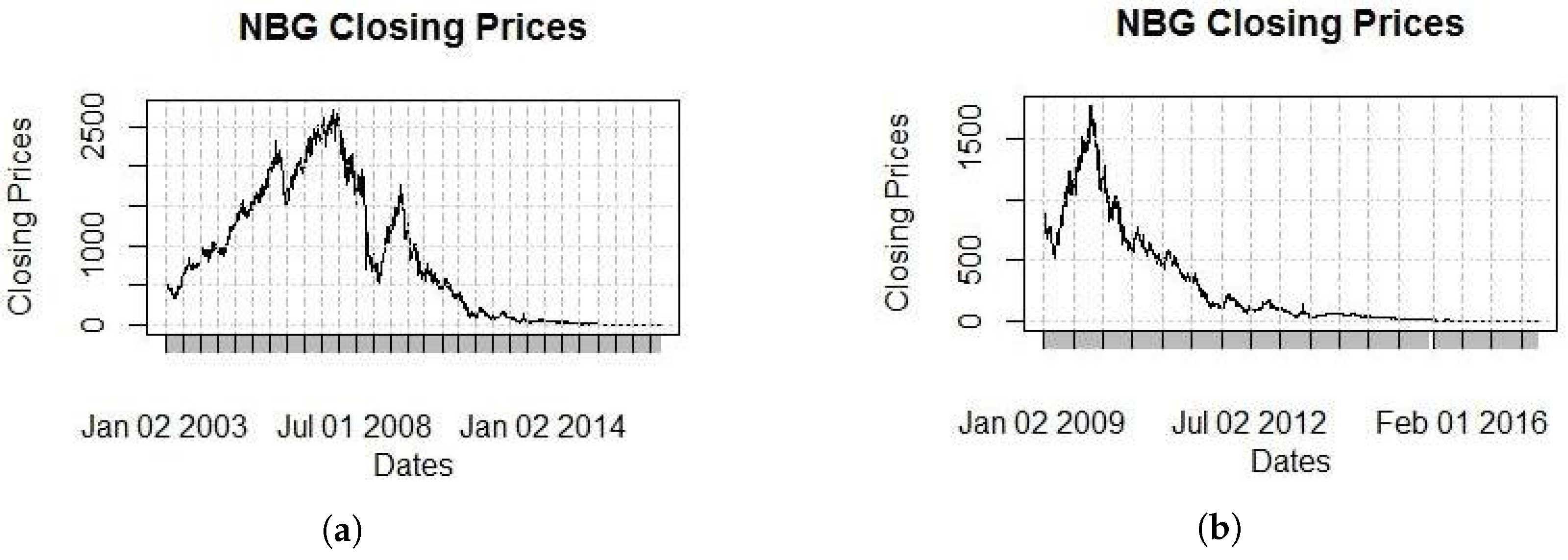
Our methodology will be implemented on the NBG stock from the banking index of the Athens Stock Exchange (ASE or ATHEX). Note that the NBG is one of the four systemic banks in Greece. Our choice emanates from the fact that it has exhibited violent changes in its price, as well as volatility structural changes because of the economic environment under which it operates. The data (7778 observations) extend for 2/1/1986 until 8/5/2017. Since such a big estimation window is inefficient, we will narrow our window to 3549 observations from 2/1/2003 until 5/1/ 2017. This choice is not completely random, as it will be clear by the plots of closing prices for five different windows provided in Figure 1, Figure 2 and Figure 3.

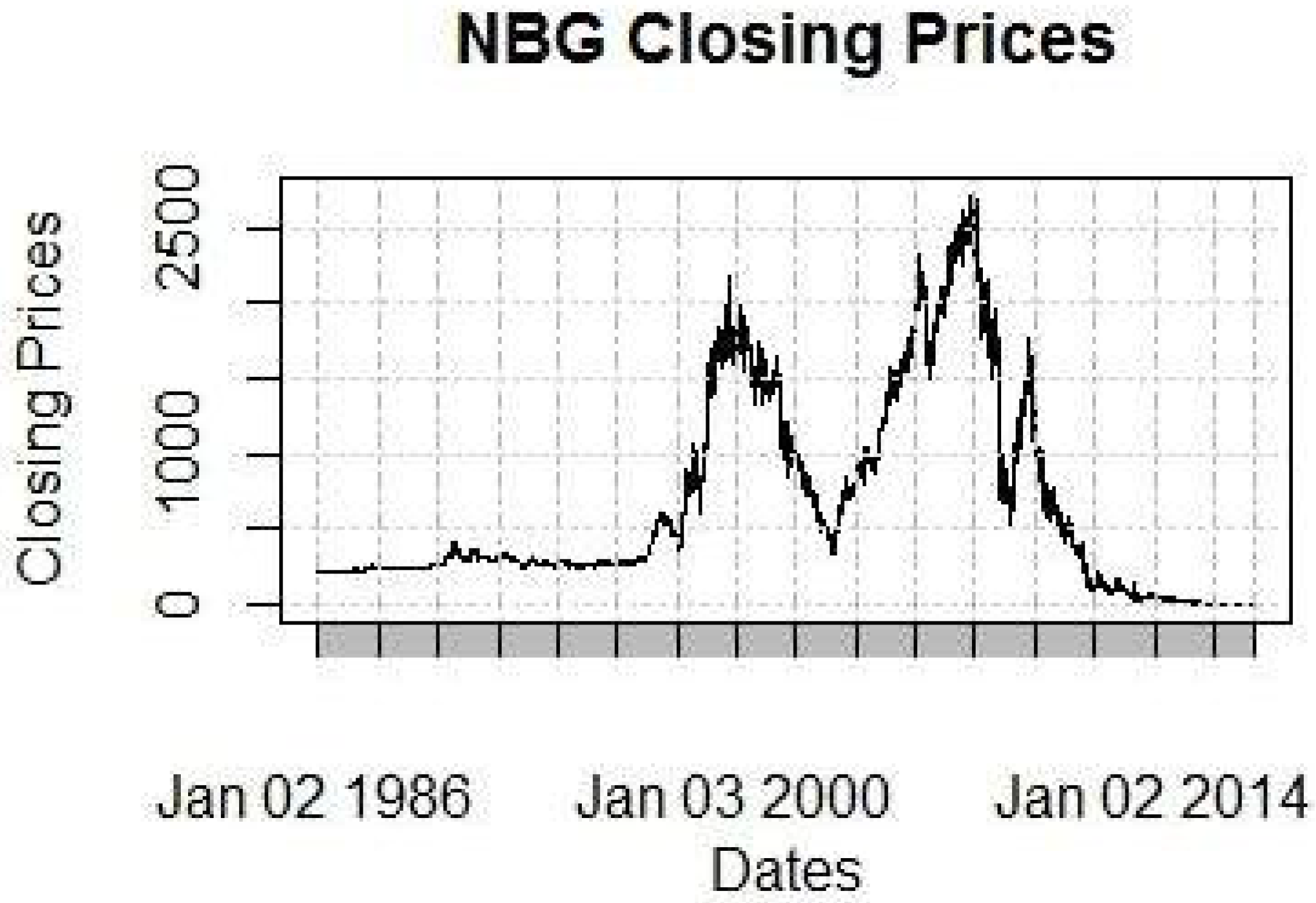
Figure 1 provides the general idea of the stock price movement over the last 30 years. Observe that prices extend to over 2000€ which is not consistent with reality. This is due to six right offerings which have been executed over the last ten years, occurring during the time periods 9/6/2006–11/7/2006, 30/6/2009–31/7/2009, 16/9/2010–27/10/2010, 13/5/2013–25/6/2013, 13/5/2014–1/7/2014 and 24/11/2015–14/12/2015.

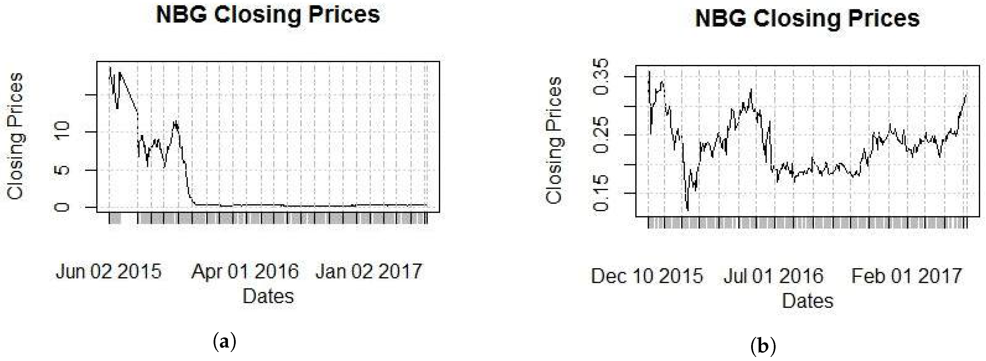
All right offerings are visible in Figure 1; in the respective periods, the prices continuously dropped as the market corrected its value. In order to get closer to the present values to be more visible, we gradually “zoom” to the present (Figure 2 and Figure 3).

All figures clearly show the impact that great economic events had of the stock price, such as the bubble of 1999, the economic crises of 2007–2009, the entrance of Greece on the IMF program on 23/4/2010 and the enforcement of capital controls on 29/6/2015. “Rare” events such as these make the aforementioned stock an ideal example for the complex models we consider below.

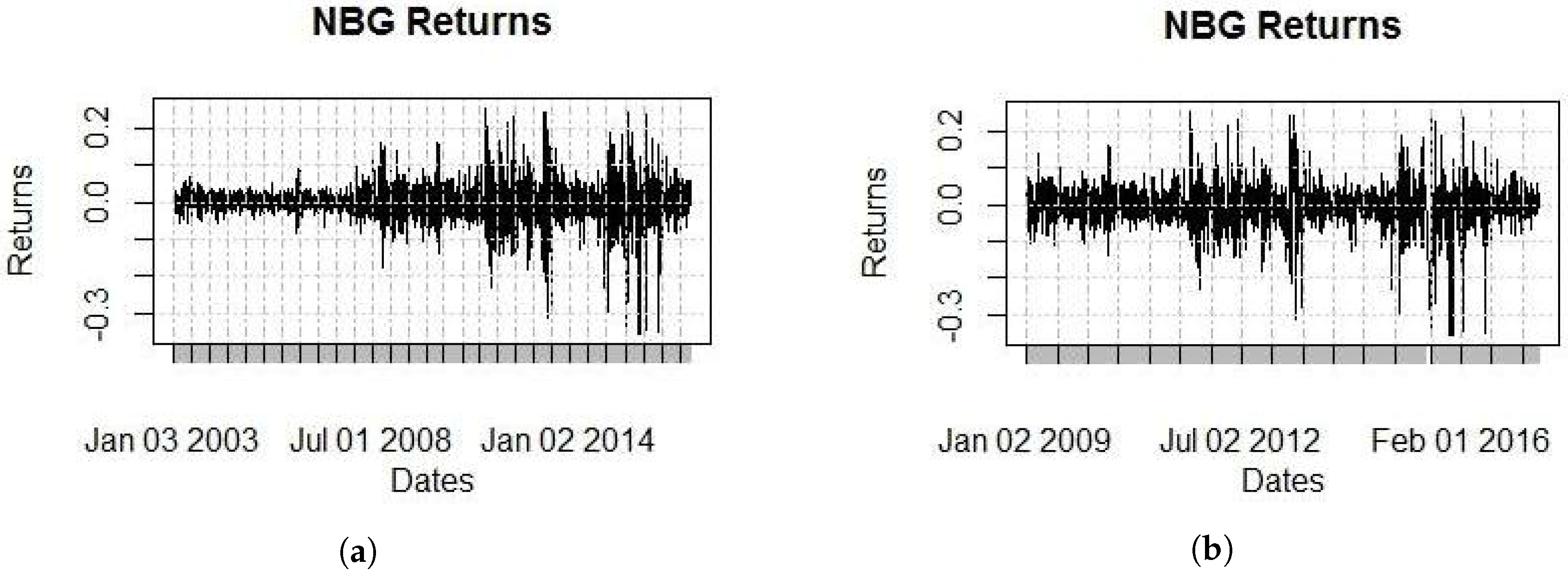
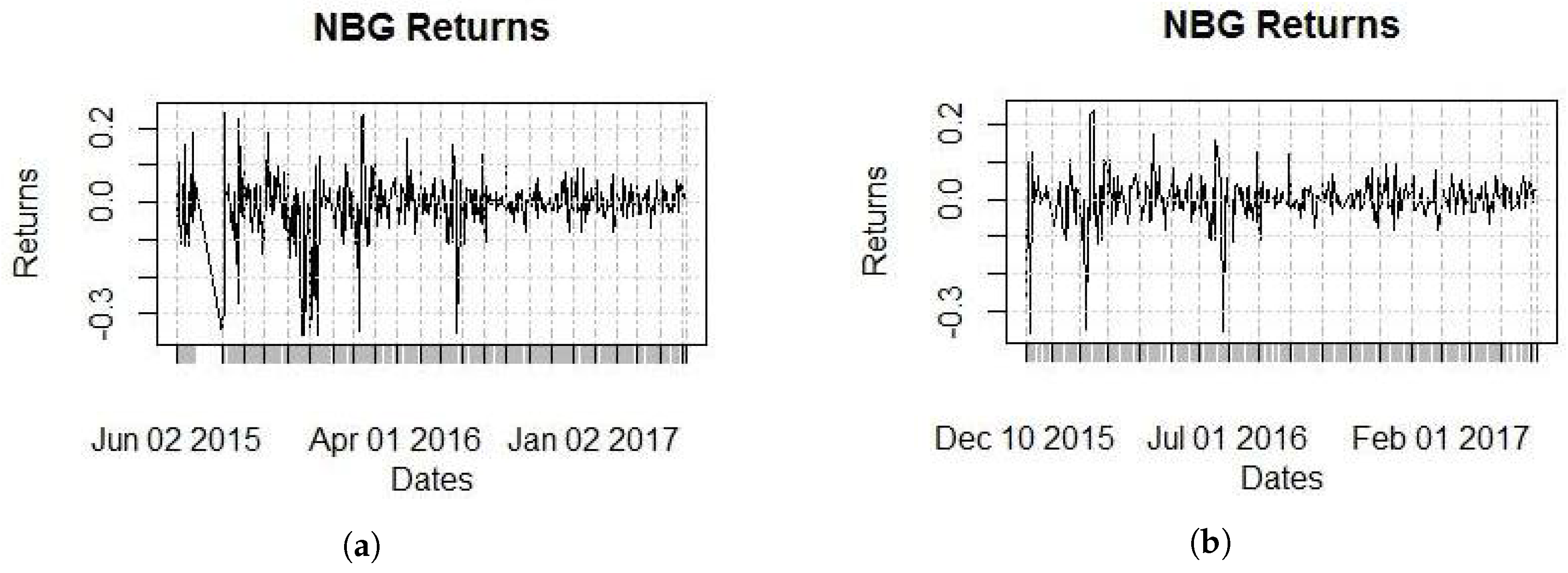
Moving our study from prices to returns, we provide Figure 4 and Figure 5 which reveal a volatility “nightmare”, not only because of the level of volatility, but also because of the clusters that are visible even to the naked eye.

The daily return mean is very small at −0.2% while daily volatility is 4.8%. The fact that the daily mean is only one-twenty-fourth of the daily volatility will simplify the construction of volatility models as we can assume that the mean is zero, without loss of generality. The returns have a negative skewness of −1.066 (i.e., negative returns are more likely to happen than positive) but more importantly, they have very high kurtosis of 14.327 (an indication of fat tails).

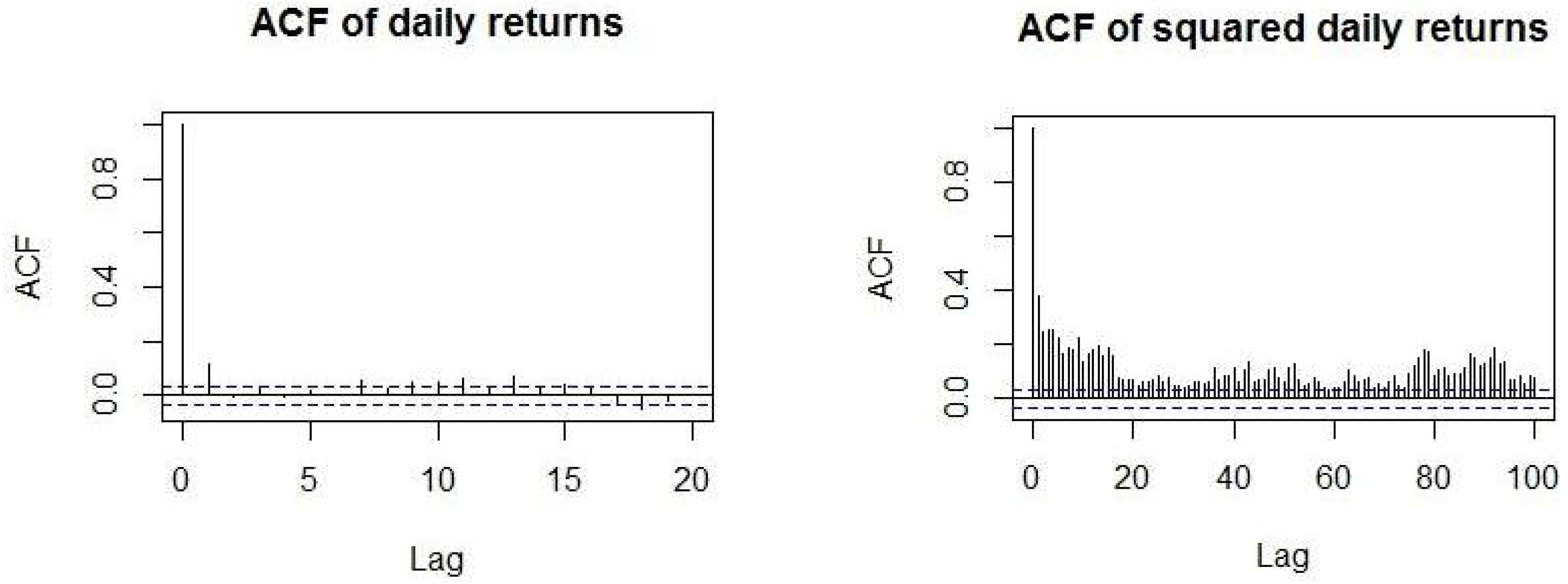
Finally, the returns have a relatively high daily autocorrelation of 12%, while squared returns (which are a proxy for volatility) have an even higher autocorrelation of 37.7%. As it was expected, squared returns exhibit higher autocorrelation than returns. The 37.7% autocorrelation of squared returns provides very strong evidence of the predictability of volatility and the existence of volatility clusters. For the latter, the Engle’s Lagrange Multiplier test for 20 lags indicates that the null hypothesis is rejected, i.e., there is no predictability in the ARCH volatility model and volatility clusters are present (test statistic = 784.94, p-value < 2.2 × 10${}^{-16}$).

We also plot (Figure 6) the autocorrelation function (ACF) of daily and squared daily returns along with the associated 95% confidence intervals for 20 and 100 lags respectively. The figures clearly show that returns are barely dependent on the return of the previous days, while on the other hand, squared returns seem to have a very long memory since even after 100 lags the correlation is still significant. This provides us with yet more strong evidence for the predictability of volatility.

The Ljung–Box (LB) test was used in order to test for the joint significance of autocorrelation coefficients over several lags. We run it using 20 lags of daily returns while using at first the full sample size (i.e., 3549), as well as the most recent 2052 and 460 observations with similar results. Results show that there is significant return predictability for all three cases. The p-value for the smallest sample size of squared returns (p-value $<4.059\times {10}^{-16}$) is lower than the corresponding value for returns. Hence, we conclude that it is easier to predict volatility than the return.

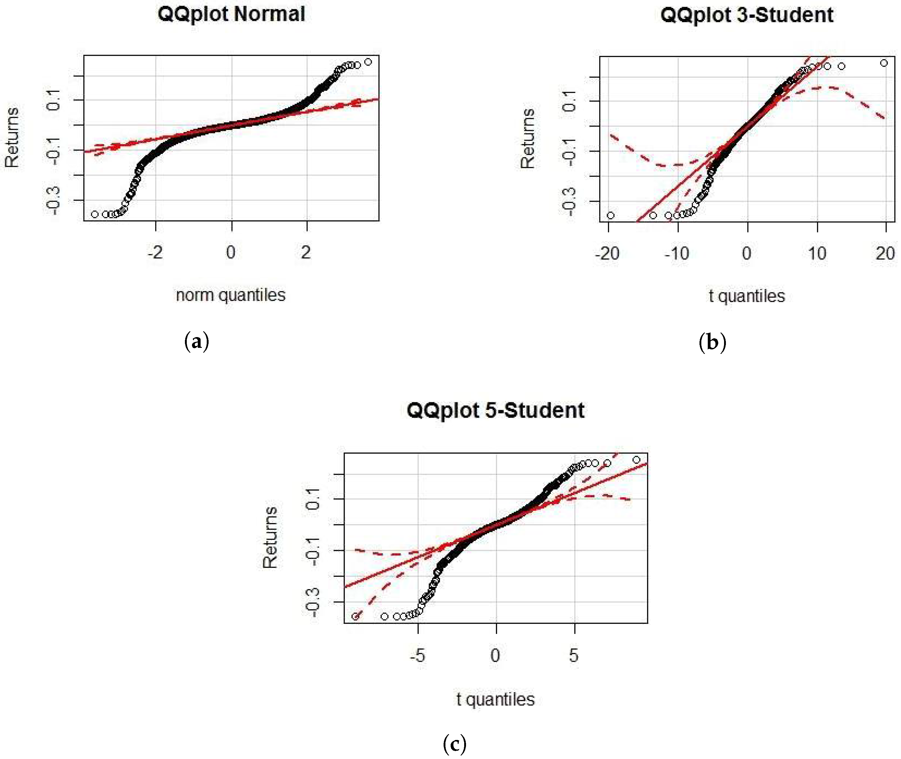
For the distribution of returns, the QQ plots for Normal, 3- and 5-Student t distributions are also furnished (Figure 7). The plots clearly show that the underlying distribution is not normal, since the tails do not fit. The deviation from normality has also been confirmed via the Jarque–Bera test (p-value $<2.2\times {10}^{-16}$). The 5-Student t distribution also seems not to have fat enough tails. Lastly, the 3-Student t distribution seems to capture the fatness of the right tail, while the left is still fatter.

We proceed now with the fitting of GARCH family models which are evaluated and compared with each other for identifying those that work better. The models considered are:

• ARCH(1), ARCH(4) and ARCH(5) with normal innovations
• GARCH(1,1) with normal and t-Student innovations
• GARCH(1,1), (4,1), (5,1), (2,2) and (3,2) with skew t-Student innovations
• APARCH(1,1) with Normal, t-Student and skew t-Student innovations and with Normal innovations and $\delta =2$,
• APARCH(2,2) with Normal, t-Student and skew t-Student innovations
• IGARCH(1,1) with and without a constant and with a constant with Student’s t innovations
• FIGARCH(0,d,0), (1,d,0),(0,d,1),(1,d,1) and (1,d,1) with Student’s t Errors

It should be noted that the data, before being fitted, were multiplied by 100 and demeaned.

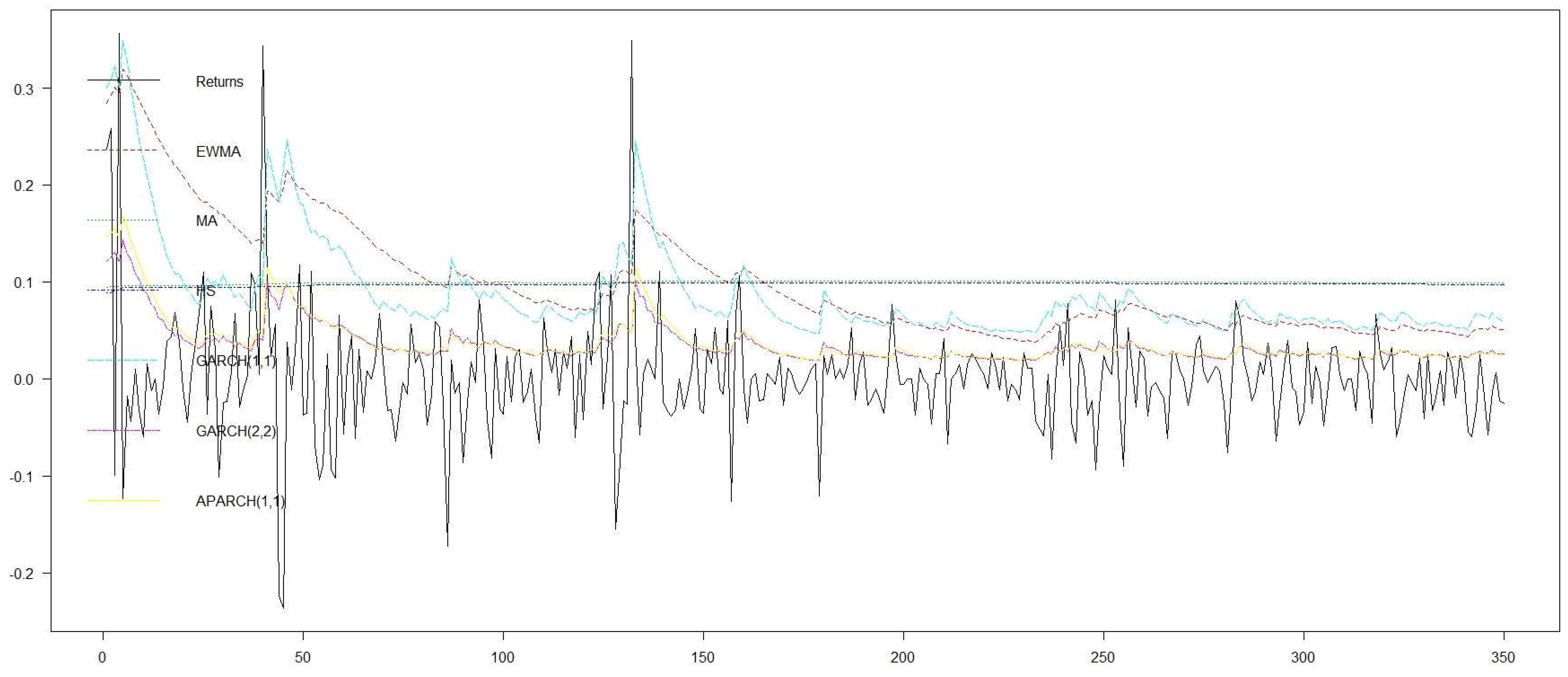
By comparing the above models using AIC and BIC (results not shown) and after we tested that all of their parameters are statistically important, we conclude that GARCH(1,1), GARCH(2,2) and APARCH(1,1) all with skew t-Student innovations are the models that appear to perform better than the rest. In order to measure their forecast ability, we implement backtesting considering, in addition to the above three best choices, the simple HS, MA and EWMA models. For evaluating the applicability as well as the effectiveness of the proposed low price effect approach, we run the models and the respective backtesting twice in the last part of the series where the threshold for the low price effect has been surpassed. This happened on 10/12/2015 leaving 349 available values until the end of the series. The results of backtesting for the two runs–one without and one with the low price correction—are shown in

Table 1. Backtest results with and without low price effect (lpe) being taken into account.

	VR without lpe	VR with lpe	VaR vol without lpe	VaR vol with lpe
EWMA	0.6285714	0.6285714	0.06026717	0.0603289
MA	0.8571429	0.7428571	0.001316615	0.002102242
HS	0.9142857	0.8	0.001710221	0.002358666
GARCH(1,1)	0.9142857	0.8	0.05176546	0.05173457
GARCH(2,2)	3.771429	3.257143	0.02092407	0.02087996
APARCH(1,1)	3.657143	3.085714	0.02497998	0.02502232

. Recall that if $mp{r}_t\ge \mathsf{\Theta }$ and $k·mp{r}_t<Va{R}_t<(k+1)·mp{r}_t$ for some $k\in Z$, then according to the low price (VaR) correction, $Va{R}_t$ is rounded to the next integer multiple of $mp{r}_t$, namely ${\widetilde{VaR}}_t=(k+1)mp{r}_t$. Otherwise, the VaR forecast remains intact, i.e., ${\widetilde{VaR}}_t=Va{R}_t$.

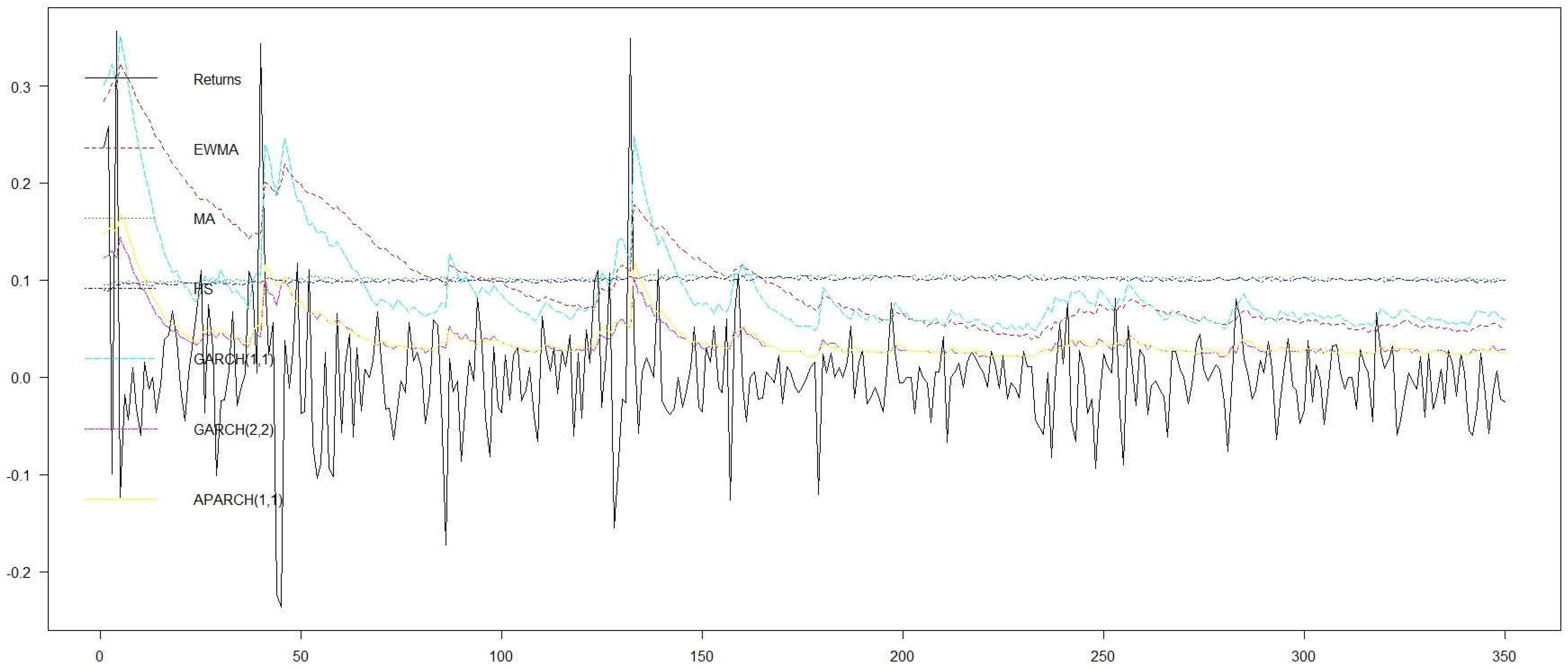
The results in Table 1 and in Figure 8 and Figure 9 clearly show that if the low effect correction is taken into consideration in backtesting, the Violation Ratio (VR) is always improved in the sense that the frequency of violations is reduced which is implying a more defensive approach in accordance with Basel III. Indeed, observe that in all cases except the EWMA model, the observed number of violations has been reduced and as a result the violation ratio is improved. As expected, the low price correction is extremely effective for failing models such as GARCH(2,2) and APARCH(1,1). In such cases, the reduction in VR appears to be considerable. On the other hand, we observe that VaR volatility fails to show any improvement by remaining almost unaffected when the low price correction is applied. Similar conclusions can be drawn from Figure 8 and Figure 9 where forecasts are reported with and without the low price correction. In some instances, it is clear that GARCH(1,1), which is one of the models that captures satisfactorily the behavior of the stock, has slightly improved forecasts when the correction has been applied. The improvement in forecasting when the low price correction is implemented, is obvious in models such as GARCH(2,2) and APARCH(1,1), that both fail considerably to capture the mechanism of the underlying process. Figures provide sufficient indications that when models tend to fail, the proposed methodology is highly effective.

4. Conclusions

In this work, we proposed a technique for improved volatility estimations by taking into consideration a low price correction via an approach which is based on asset prices and, as it turns out, is both simple and straightforward. The VaR estimations either remain unaffected or are improved in the sense that their violation ratio is improved. Among the advantages of the proposed method is that it is versatile since it can be applied to any risk measure and any estimating method chosen by the investigator while it does not require estimation of any extra parameters. Furthermore, it should be pointed out that the violation ratio was always improved in all scenario simulations considered as opposed to VaR volatility that did not seem to be affected. Although it is always useful, as expected, it is extremely useful and powerful in extreme scenarios and severe stock collapses.

Through the proposed methodology, we fill the gap in the relevant literature and provide evidence that prices could contain additional (to the amount contained in returns) important information which, if used shrewdly and properly, could be advantageous for risk estimation. Last but not least, we also provide the solution to the problem. The asset under consideration must be reverse splitted if possible in order to correct the above problems.

Apart from any theoretical considerations, the practical implications that the low price correction entails are the key issues in the contributions of the present work.