
A Cointegrated Regime-Switching Model Approach with Jumps Applied to Natural Gas Futures Prices


1
Chair of Financial Mathematics, Technical University Munich, 80333 München, Germany
2
Department of Mathematics and Statistics, University of Calgary, Calgary, AB T2N 1N4, Canada
*
Author to whom correspondence should be addressed.
†
These authors contributed equally to this work.
Risks 2017, 5(3), 48; https://doi.org/10.3390/risks5030048
Submission received: 24 July 2017
/
Revised: 30 August 2017
/
Accepted: 7 September 2017
/
Published: 12 September 2017
Abstract
:Energy commodities and their futures naturally show cointegrated price movements. However, there is empirical evidence that the prices of futures with different maturities might have, e.g., different jump behaviours in different market situations. Observing commodity futures over time, there is also evidence for different states of the underlying volatility of the futures. In this paper, we therefore allow for cointegration of the term structure within a multi-factor model, which includes seasonality, as well as joint and individual jumps in the price processes of futures with different maturities. The seasonality in this model is realized via a deterministic function, and the jumps are represented with thinned-out compound Poisson processes. The model also includes a regime-switching approach that is modelled through a Markov chain and extends the class of geometric models. We show how the model can be calibrated to empirical data and give some practical applications.
1. Introduction
The physical and the financial markets of energy commodities have converged over time. This is shown in multiple studies, e.g., Adams and Glück (2015), Benth and Koekebakker (2015), Carmona (2015), Döttling and Heider (2014) and Silvennoinen and Thorp (2013). The phenomenon itself is based on the increasing liquidity of energy markets. On the one hand, many banks are looking to benefit from investments in commodity derivatives, and on the other hand, there are more and more traded products. As a matter of course, an increase in liquidity usually causes an increase in the volatility of prices; see (Brunnermeier and Pedersen 2009). The natural reaction of companies that suffer from price volatility is to hedge. This leads to further developments in the markets such as new derivatives. However, the most commonly-traded financial instruments in commodity markets remain futures and options; see (Geman 2009). Nevertheless, most financial models dealing with commodities use spot prices even though these prices are often estimates. On the other hand, hedging still requires a highly suitable model for the prices under consideration. Furthermore, there are multiple models covering especially the nature of natural gas prices, e.g., Andersen (2010). Over the last few decades, mean-reverting models (e.g., the Ornstein–Uhlenbeck (OU) process) have been the most common for commodity prices; see (Schwartz 1997). Newer developments include multivariate models in order to model correlations, several underlyings or stochastic parameters such as stochastic volatilities. Multi-factor mean-reverting models with jump-diffusion are for example used for both electricity and gas spot prices by Meyer-Brandis and Morgan (2014). Other recent approaches to modelling gas markets are infinite-dimensional models for forward markets proposed by Barndorff et al. (2015) and Benth and Krühner (2015).
If one thinks of futures, one also has to think of their maturities. Naturally, the question of the interdependence of futures with different maturities arises. Empirical data analysis shows that these futures are not only correlated, but also cointegrated; see (Chowdhury 2006). Most of the time, cointegrated models in mathematical finance deal with the cointegration between different underlyings. Daskalaki et al. (2014) look at monthly and quarterly return data for a collection of individual commodities, and Kavoussanos et al. (2014) examine volatility spillovers between commodity and freight markets and the existence of a long-run equilibrium (cointegration) relationship between them. Zhang and Qu (2015) explore cross-market cointegration in China’s agricultural commodities due to global oil price shocks. Batchelor et al. (2007) investigate the relationship between the spot and the nearest-dated forward price in the international freight market employing ARMA and VAR models and cointegration tests. Panagiotidis and Rutledge (2007) document that there exists a cointegrating relationship between the gas and oil price in the spot and futures markets. However, none of these papers try to model the joint evolution of the forward curves. At best, they look at the relation between the spot price and the nearest-dated futures price. Farkas et al. (2016) propose a system of cointegrated commodity prices and allow for an arbitrary number of cointegration relationships. They derive futures prices as a derivative of the underlying commodity, thus excluding jumps, which are specific to only one future of a given maturity or a subset of traded futures with different maturities. Therefore, one question we address in this paper is whether one can find a model that covers the cointegration of futures with different maturities and different jump behaviours.
Typical models that are used to model commodity prices and commodity-based financial products are based on geometric or arithmetic models (Benth et al. 2008, p. 59 ff). Both of these model types use Ornstein–Uhlenbeck processes to model commodity prices and a multi-factor approach. Other known multi-factor models that are used to analyse the price structure of commodities include the stochastic long-run mean model by Pilipović (2007) and the stochastic convenience yield models by Schwartz (1997), in which one-factor, two-factor and three-factor models are considered. This paper also includes the two-factor Gibson–Schwartz model where one factor is the spot price and the other one is the instantaneous convenience yield. One stylized fact that motivates the use of multi-factor models is the stochastic change in the shape of the forward curve; while shifts (sometimes sudden) in the whole curve occur, we also see more complex behaviour that cannot be captured by a single factor. For storable commodities, prices for delivery times that are close together are relatively highly correlated. Further, for some commodities such as natural gas and electricity, anticipated cyclical factors affecting demand generate corresponding cyclical patterns in the levels of futures prices. Another observation (pertinent to the approach in our paper) is the appearance of qualitatively different dynamical behaviour at different times, possibly corresponding to unanticipated changes in market conditions. Schwartz and Smith (2000) have analysed commodity dynamics in a different setting using short- and long-term factors. They prove that this model is equivalent to the Gibson-Schwartz model. Several other approaches generalize the models above including Casassus and Collin-Dufrense (2005) and Nielsen and Schwartz (2004). The model of Paschke and Prokopczuk (2009) considers cointegration in a commodity futures context. This model is based on the class of geometric models and uses cointegration to model prices of different commodities while also including jumps. We want to mention here that multi-factor models based on Ornstein–Uhlenbeck processes can lead to cointegration or in the case that the number of underlying risk-factors is smaller than the number of observed time series, directly enforce the assumption of cointegration.
The aim of this paper is to find and discuss a suitable model for a considered commodity and its futures prices that is able to incorporate cointegration of the term structure. With the integration of this feature, the model can describe the development of the term structure over time and hence also allow for a simulation of the term structure in time. Moreover, the number of underlying risk factors can be reduced since the information, which is needed to model the term structure, is inherently provided through the structure of the model. Nevertheless, we include the basic requirements of a common commodity model. The proposed model can be viewed as an extension of the Schwartz–Smith model. Cartea and Williams (2008) considered an extension that includes seasonality in a similar way to this approach. The model shall allow for different jump behaviours of the future prices of different maturities. Shortage in supply and demand might lead to joint jumps in prices until shortage is eased, while individual jumps are highly typical for commodities that cannot be stored or easily produced. The model shall also allow for different behaviours in different market regimes.
First, we take a deep look at prices of futures that are traded at the Intercontinental Exchange (ICE) in Section 2. We observe that the prices are cointegrated, have strong seasonal effects, incorporate jumps and also depend on different regimes based on volatility. In Section 3, we formulate and propose a model that incorporates these effects and show how one can use the Kalman filter in order to calibrate the model to market data. Furthermore, the goodness-of-fit is analysed. Finally, we show applications of the model (Section 4).
2. Data Analysis and Stylized Facts
In the following steps, we want to analyse commodity futures in order to develop a suitable model for highly correlated commodity futures prices of one underlying commodity with different maturities. We use rolling futures prices of the ICE U.K. Natural Gas provided by Bloomberg (the expiration date is two business days prior to the first calender day of the settlement month). These are futures with the maturities from 1–5 months (Bloomberg ticker: FN1, …, FN5). The reason why we want to use natural gas futures lies in several effects like seasonality, which are not always observable for other commodities like crude oil; see (Schwartz 1997). We observe data of these futures in a timespan from August 2003 until the end of July 2013 (Figure 1).
As a first step, we compute the correlation matrix of the futures prices. The values are displayed in Table 1 and show that these prices are highly correlated.
The most important conjecture we want to analyse here is the one that the data are not only correlated, but also cointegrated. Hence, we test the data for cointegration. The test we will use first is the Engle–Granger test; see (Engle and Granger 1987). Engle–Granger tests assess the null hypothesis of no cointegration among different time series. Let h be the Boolean decision variable for the test. A value of h equal to one (true) indicates rejection of the null in favour of the alternative of cointegration. Values of h equal to zero (false) indicate a failure to reject the null. For the considered data, we can reject the null with a p-value of 0.001 suggesting the cointegration of the futures.
As a second, more modern test, we will use the Johansen test; see (Johansen 1991). The Johansen test assesses the null hypothesis H(r) of the cointegration rank less than or equal to r. Hence, this test gives us a suggestion of how many underlying risk factors we have to consider in a multi-factor model. The results of this test are displayed in Table 2 and suggest that the data are cointegrated with rank . A cointegration of rank is rejected. In Table 2, the “H(r)” denotes the null hypothesis, the “Stat” means the test statistics, and the “eigVal” means the eigen value associated with H(r).
Having in mind the cointegration of the futures prices, we now want to state other effects that we have found by analysing the data. An overview of typical effects for gas futures can be found in Benth et al. (2008) (p. 129 ff). These effects are seasonality, jumps and a regime-switching behaviour.
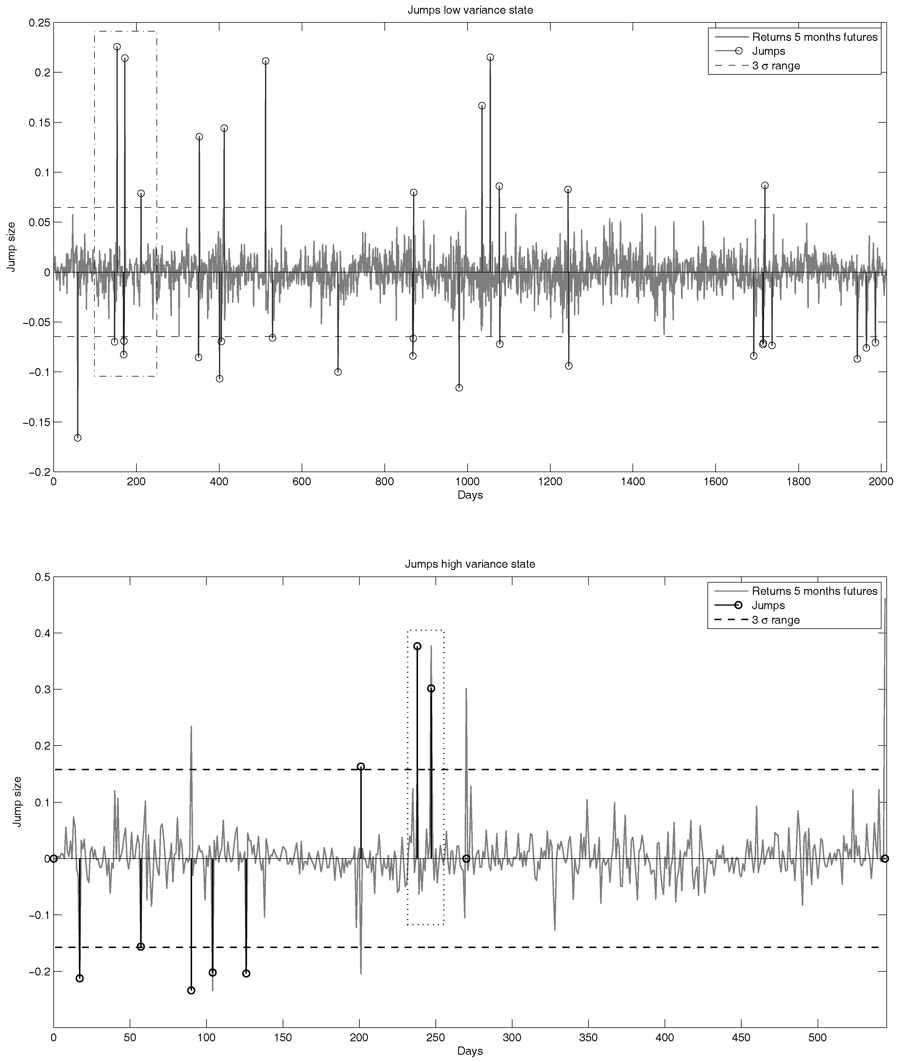
Seasonality occurs within the cycle of one year comparable to other energy commodities driven by demand. Jumps on the other hand can either appear simultaneously within all time series at once or only within a subset of the futures. Usually, these jumps are related to political or social crises. One example are jumps we observe in August 2006, where Israel started a ground offensive in Libya, and a diplomatic solution was close to failure (marked with a dotted/dashed square in Figure 8). Another example for jumps can be found around Christmas in 2011 after heavy suicide bombings in Syria and Afghanistan (marked with a dotted square in Figure 8). The regimes, which are based on volatility, can be linked to more general effects in the financial markets. One example for a high volatility regime is of course the financial crisis. Following our data analysis, we want to develop a model that includes seasonality, regime-switching effects and jumps. We proceed with a further analysis of the data and state the functions/stochastic processes we use to model the above effects. Furthermore, we estimate the model parameters using market data. Finally, we state the model, which results from this analysis.
Since we want to ensure non-negativity in our model, we continue with the log-prices of the observed futures data. We now proceed by filtering the seasonality component from the data giving us a deseasonalized data series. In a next step, we split the data series into a low and a high volatility state. This is done because we can expect a different jump behaviour in a low and a high volatility state due to different volatility and skewness. We then filter the jumps of the two data series and calibrate the jump processes. In the last step, we subtract the jumps, and the two “smoothened” times series are used to calibrate the geometric model. Taking this approach has several implications on the observed jump behaviour and the estimated parameters of the geometric model. We will state the details of these effects in the following subsections.
2.1. Seasonality
We now filter and model the seasonality of the data series. In order to filter seasonality and obtain an empirical, deterministic, periodical seasonality function, we follow the instructions of Brockwell and Davis (2002) (p. 179 ff). This method is based on averages over the observed time horizon in the same period every year on a daily basis. This smooths the seasonality function over the observed years and enables it to return a seasonal factor for each day on a one-year horizon. The estimated seasonality function for each future is given by:
where is the log return of future l at time t and is the number of observed years (we account for 250 trading days each year). We furthermore assume that this seasonality function stays constant over all observed years, meaning that we repeat this estimation for all years. The results of this filter are shown in Figure 2 and Figure 3. As one can observe, the seasonality manifests as a yearly, periodic function that reflects the global demand on gas. We use this function to clear the seasonality effects of the time series. This allows us to observe the movement of the time without these effects, focusing on the underlying stochastic processes.
2.2. Regime-Switching
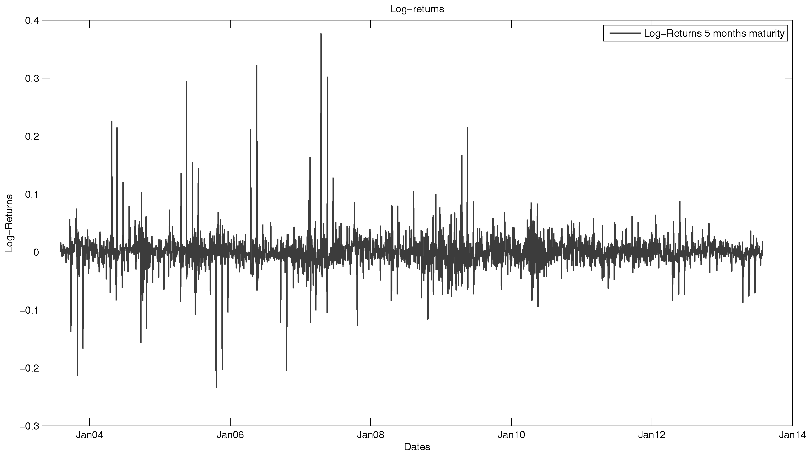
In a next step, we will observe the seasonality-adjusted log-returns of the natural gas futures. As one can see in Figure 4, the historical volatility of the futures varies between states with high volatility (for example, during the financial crisis) and states with low volatility.
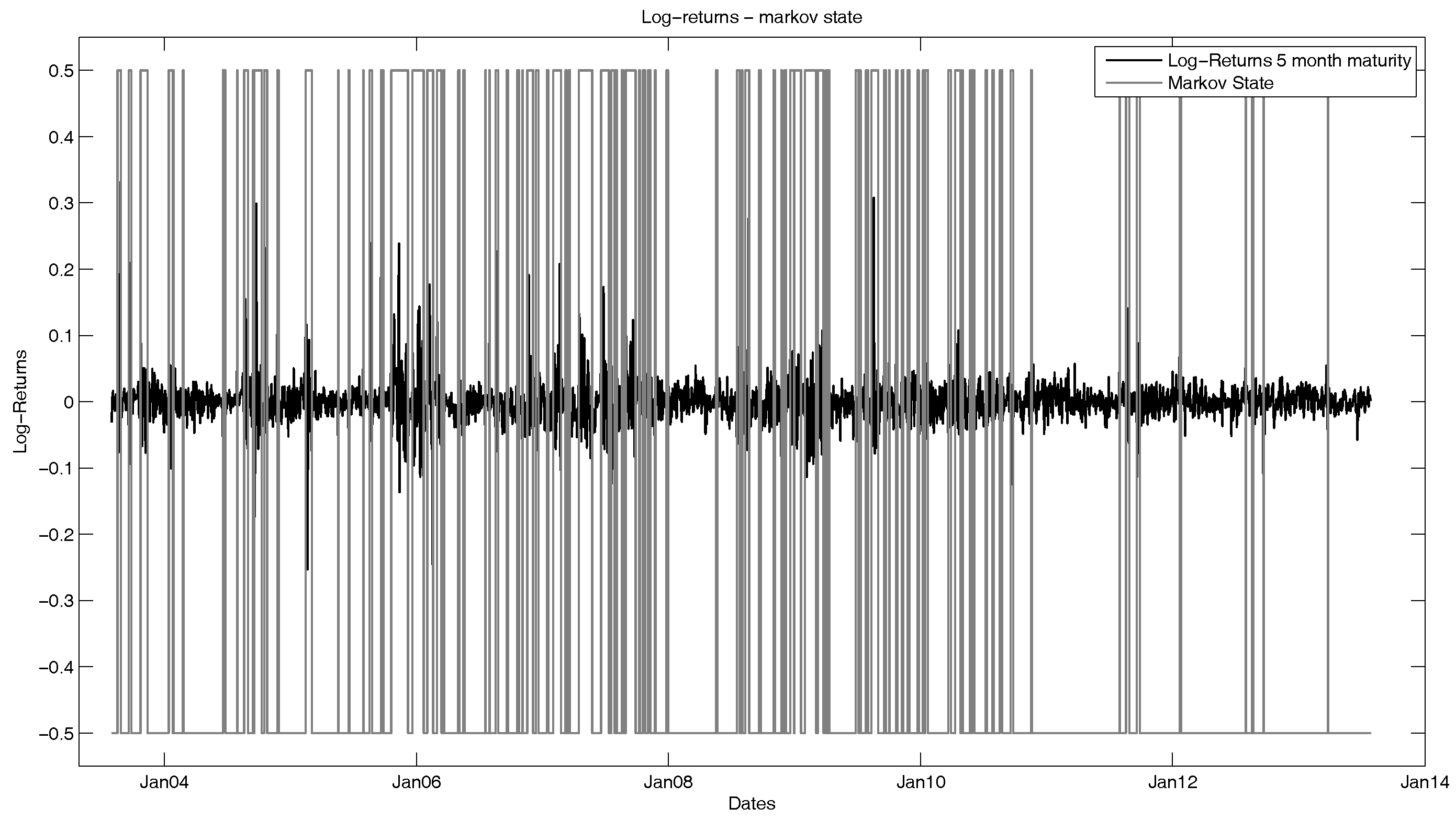
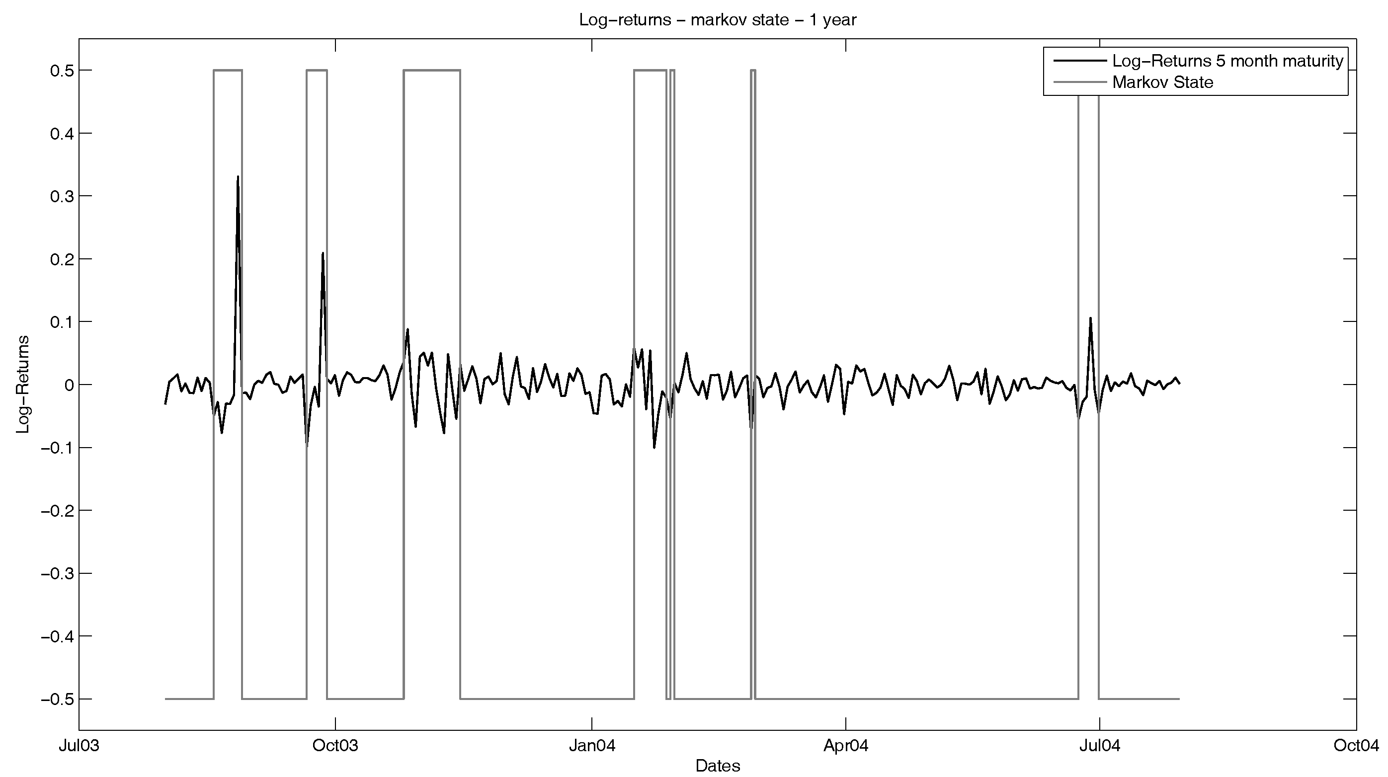
In order to describe this phenomenon, we choose a Markov switching framework. The idea is to model the log-futures prices by a linear combination of the seasonality function and a regime-dependent factor process following a multi-dimensional mean-reverting jump diffusion. For simplicity reasons and the computational effort that is needed in higher dimensions, we consider a two-state Markov chain. For the estimation of the Markov states, we use the MS_Regress package in MATLAB, which computes the Markov regimes via a maximum likelihood estimation and is capable of multivariate input, meaning that the estimation is fitted simultaneously for all time series that we consider. The results of this are shown in Figure 5 and Figure 6 with the returns of the five-month future.
From this estimation, we can calculate a discrete transition matrix of the Markov chain, which gives us the probability to switch from one state into the other one. We denote the transition matrix by , where the low volatility state corresponds to State 1 and the high volatility state to State 2, respectively. The values can be found in Table 3.
The result of our calibration is that we can separate the time series into two states. As stated above, these states highly depend on effects in the financial markets and are based on volatility. The Markov transition matrix can be interpreted in the following way: The regime of the time series changes with a probability of 1.5% from the low to the high volatility state and changes from the high to the low volatility state with a probability of 3.4%. This means it is more than twice as likely that the time series switches to the low volatility state, and the probability to remain in State 1 is 98.5% compared to 96.6% to stay in State 2. Hence, the time series in general are more likely to be in the low volatility state. Nevertheless, the time series stays in the state in which they are at the observed point in time with a very high probability.
2.3. Jumps
From now on, we will always consider the time series for the two separated states. In a next step, we want to include jumps in our model for each state. We consider returns that are bigger than three standard deviations as jumps. This means for a daily log return of the futures , we consider this return to be a jump if:
where
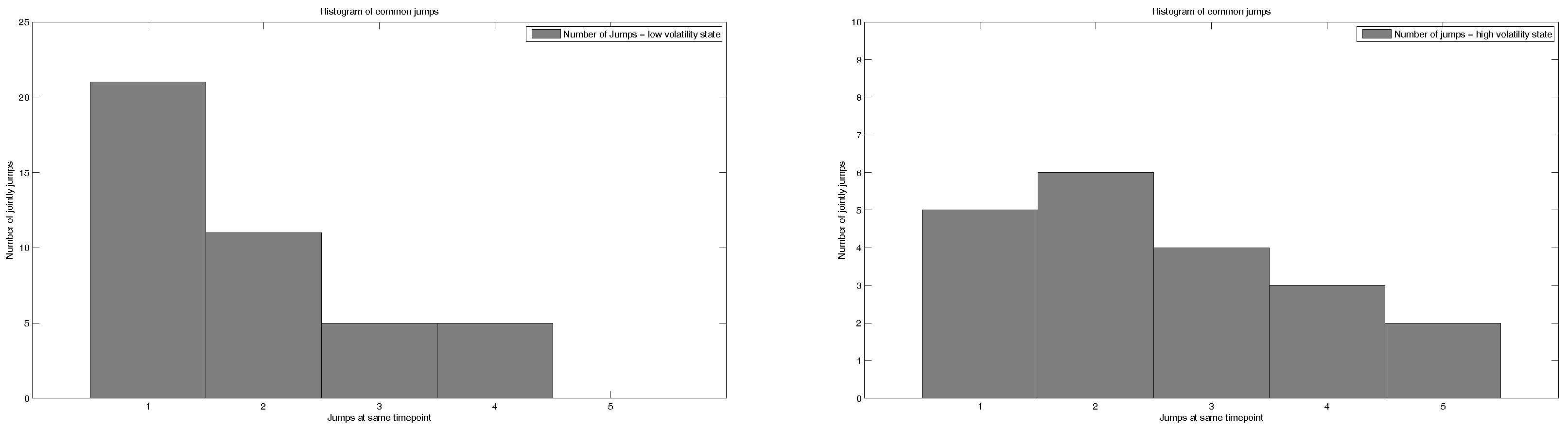
Important to notice at this point is the fact that these jumps are not independent. One can see this in Figure 7, where the number of jumps is displayed that happen in a five-day window. We want to note that we observe more jumps in the low volatility state due to the price skewness. Here, one can see that there are extreme events in which all time series jump at once. Furthermore, the other jumps do not happen independently. Hence, we will model the jumps in two processes. One process only tracks the extreme events. The other jump process will model the jumps with thinned-out compound Poisson processes. We filter the detected jumps from the data and go on with the cleaned time series. Using such cleaned data series reduces the volatility that is observed calibrating the underlying geometric model.
As one can see in Figure 8, the jumps during the high volatility state are (absolutely) bigger than the jumps during the low volatility state (average for the low volatility state: 0.11; average for the high volatility state 0.14). The higher probability that a jump occurs in a low volatility state is due to the fact that the average standard deviation in this state is lower, and therefore, smaller outliers are considered jumps.
3. Model and Calibration
3.1. An Extended Geometric Model
Now, we adapt a geometric model in order to include the discussed and observed stylized facts, which are seasonality, jumps, regime-switching and cointegration. Compared to other models that are usually used to describe commodity prices, we not only include the basic effects such as seasonality and jumps, but also the regime-switching approach and cointegration. Both of these effects are rather unusual for commodity models, but as the data have shown, both effects can be observed within the analysed natural gas futures. Compared to the model of Paschke and Prokopczuk (2009), which includes cointegration, we also include jump-effects and regime-switching. Furthermore, the model we want to state now models not only different commodities or multidimensional time series, but also the term structure due to the considered cointegration.
At this point, it is important to notice again that we want to model multidimensional data. This means that the price process of the futures and the process of the underlying risk factors (we use this dimension for the risk factors since we have seen before that the time series are cointegrated with rank ); also, we consider a jump process for each future, meaning that . Furthermore, we consider the seasonality function independent of the Markov chain , which introduces the different states of the model. We can now state the model as follows:
where:
is assumed to be diagonal. and are the matrices in order to introduce cointegration. denotes a three-dimensional Brownian motion. The processes are thinned-out compound Poisson processes. We assume this through the histograms (Figure 7) we have shown before. Here, we can see that it is most likely for the processes not to jump at the same time, even if this is possible nevertheless. We want to take this phenomenon into account by choosing the components of as:
where is a Poisson process with rate and is a Bernoulli process with:
Furthermore, are independent and identically-distributed processes. We assume that are normally distributed with .
The processes model the jumps at extreme events. Hence, we define them as compound Poisson processes that jump at the same time. This means the components of are:
where is a Poisson process with rate and are independent and identically-distributed processes. We assume that are normally distributed with .
3.2. State Space Form and Calibration
The next step is to calibrate the underlying OU processes, as well as the matrix Ω, which transfers the risk factors to the modelled log futures prices. To calibrate this core part of the model, we will use the Kalman filter. In order to be able to apply this approach, we first have to take a brief look at the state space form of the “pre-filtered” model. This means that we consider the above stated two-state separated time series where we first filtered out seasonality, split the time series into two separated time series according to the state of the Markov chain and remove the jumps. The parameters of this can be found in Table 6.
We can simply derive the state space model via the discretization of the model after filtering the data according to the above-stated method. The state space model then takes the form:
Measurement equation:
where , serially uncorrelated, and .
Transition equation:
where:
3.3. Optimization of the Maximum Likelihood function
The calibration of the model is done by using a Kalman filter and optimizing the resulting maximum likelihood function. A solution to this optimization problem is derived in different steps. For the basic setup, we use the “dlm”-package in R (Petris et al. 2009). This package is able to build a Kalman filter of the model and can evaluate the maximum likelihood function. For the optimization itself, the “optim”-function in R is used along with several optimization techniques. The method that was most effective and stable in our test is the Broyden–Fletcher–Goldfarb–Shanno method (BFGS-method). In the following Algorithm 1, one can find a schematic display of the optimization.
| Algorithm 1 Calibration of a geometric model. |
| Choose a random starting parameter set . |
| Separate in subsets . |
| Set the outer optimization control parameter to a random high number. |
| while do |
| for all to n do |
| Set the inner optimization control parameter to a random high number. |
| while do |
| Run Kalman filter for the parameter set . |
| Optimize the MLE resulting from the Kalman Filter for , and receive . |
| Set . |
| Set = . |
| end while |
| Set = . |
| Update with the new parameters from . |
| end for |
| end while |
3.4. Estimated Parameters
In Table 4 and Table 5, we state the estimated parameters for the underlying risk processes that we estimated via the Kalman filter and the maximum likelihood estimation, respectively. Please note that the futures and their respective parameters are sorted by their maturities linking, e.g., the first row of the matrices and to the one-month future. In the parameters of the matrix , we can see the influence of the three considered risk factors on the futures time series. The matrix gives us indicators of the cointegration and the linear independences of the risk factors since its structure reflects the cointegration of the futures. This means that the obvious linear independence of the columns (rows) of this matrix indicates that the risk factors reflect different influences on the futures prices. Such influences can be a general drift or connections between futures with short- and long-term maturities, respectively. This also allows for the modelling of contango and backwardation1 (rising or falling forward/futures curve). gives us an idea of the mean-reversion level of the risk factors.
First, we want to take a look at the low variance case. Here, we can see that the third risk factor is the most influential. Since is the largest -component, this means that the third risk factor is used for the drift of the time series. Hence, the other risk factors are disturbances that calibrate the cointegration of the series and the structure of the forward curve. As we can see in Table 5, these two risk factors are also the most volatile. The structure of (considering the signs, namely that for the first column, the first and last entry are negative, for the third column, the first and second entries are negative and for the last column, the last two entries are negative) tells us that the risk factors are independent, which was also calculated in MATLAB (rank () = 3).
In the high variance case, on the one hand, we have a similar picture. Here, the second risk factor is used for the drift. On the other hand, the factors are all clearly independent (considering the structure of again by the distribution of negative entries: first column with three negative entries, second with two and last column with only one negative entry). Here, the drift factor is quite volatile. Furthermore, the errors shown in Table 5 are higher than in the low variance case.
and terms give us some information about the volatility of the process. While is the measurement error that is needed to compute the Kalman filter, gives us information about the volatility of the underlying risk factors. This volatility seems to be quite low at first glance, but since this is equal to a daily volatility, already accounts for a large proportion of the overall movement of the process. As expected, the volatility is on average higher in the high volatility state (.
In conclusion, one can say that the estimated parameters we received by calibrating the model give it much structure. Due to the structure of and the structure of , we can see that the basic hypothesis of cointegration seems to be valid for the observed data.
In Table 6, the parameters for the thinned compound Poisson processes are listed. Furthermore, in Table 6, we can see the parameters for the extreme events, meaning that all time series jump at the same time. As one can see, there are no such extreme events in the low volatility phases. The first thing we want to remark on here is that the jumps in the extreme case (processes jumping at the same time) are higher on average than for the thinned-out compound Poisson process. Nevertheless, the standard deviation is lower. This is the case due to an increased rarity of these events.
3.5. Goodness-Of-Fit
The fit of the estimation can, e.g., be observed by the convergence of the simulation. By the structure of the underlying risk factors, several experiments with different optimization and calibration methods (other than the Kalman filter) resulted in diverging simulated paths, which is also the case by considering fewer degrees of freedom (DOF) in the optimization. Therefore, we also tested a structure in the parameters of the model, e.g., we assumed the matrix to be diagonal or that the first entry of is zero. Such assumptions are for example made in Paschke and Prokopczuk (2009). With less DOFs, the optimization routines, which were used in R, do not converge any more. Hence, we do not compare the fitted structure with similar processes (for example, with independent risk factors). Nevertheless, we now state some measures for the real processes and simulated processes. Furthermore, we show that the jumps, the Markov-switching and the seasonality function improve the basic model. This is done by a comparison of the value-at-risk that is computed and shown in the next section.
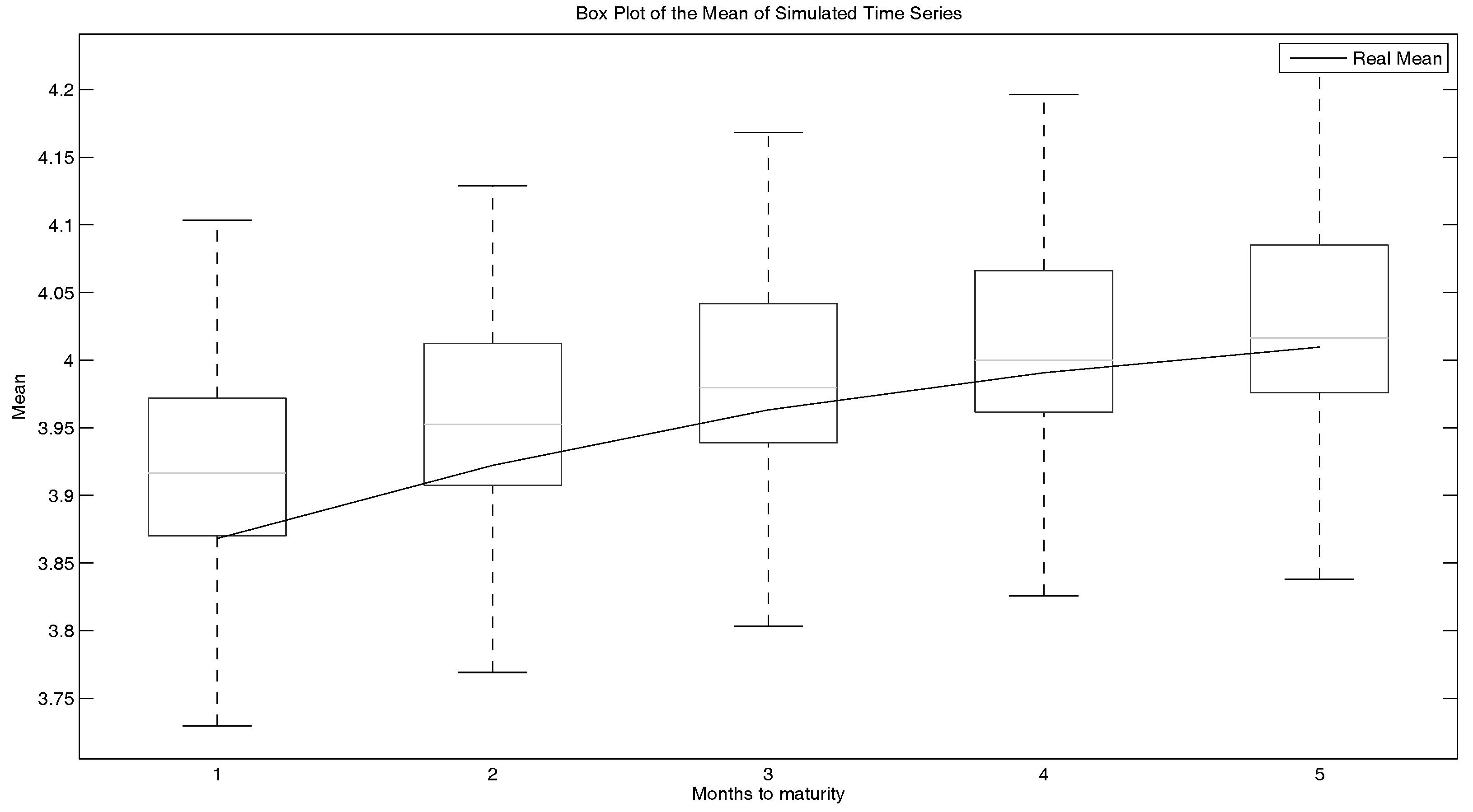
First, we look at the mean of the real log-prices of the futures, as well as of the simulated ones. In Figure 9, a box plot of the mean of the simulated time series is shown. One-hundred time series were simulated. The inputs were two years of data from August 2011–July 2012. Furthermore, the real means are shown in this plot (note that the edges of the boxes in a box plot are the 25%- and the 75%-percentiles, respectively). This plot shows that the simulated processes fit the real ones in this matter quite nicely.
We want to show this plot also for the standard deviation and the skewness. This is shown in Figure 10 and Figure 11. We can see that the fit for the standard deviation is still quite good. Nevertheless, it gets worse for the skewness.
To be more specific, the mean is slightly overestimated with this model. The standard deviation is also slightly overestimated, but still within the boxes of the box plots. However, the skewness is underestimated. One has to notice the change of signs within the skewness of longer running futures and the rising skewness. This behaviour also takes place in the simulated time series and is reproduced by the model.
We also want to compare this model to a basic geometric model without jumps, seasonality and regime-switching. This is done in Section 4. Nevertheless, we want to state, at this point, that the comparison to other models is not always given, since this model is focused on the term structure of the futures due to its incorporated cointegration.
4. Application
In this section, we analyse a possible application that the calibrated model offers. Moreover, we want to compare the model with the basic underlying model, i.e., the model without seasonality, jumps and the Markov switching framework. As an application, we will look at the value-at-risk (VaR2) that we can observe with this model. Since this type of model can diverge if the calibrated parameters are not well fitted to the observed time series (see (Karatzas and Shreve 1991), p. 281 ff), we can get an empirical indicator of how well the parameters are calibrated. We observe this via the Monte Carlo simulation we use for the VaR estimation. We run 10,000 simulations with the estimated parameters of the model. The simulated series do not diverge in any case3.
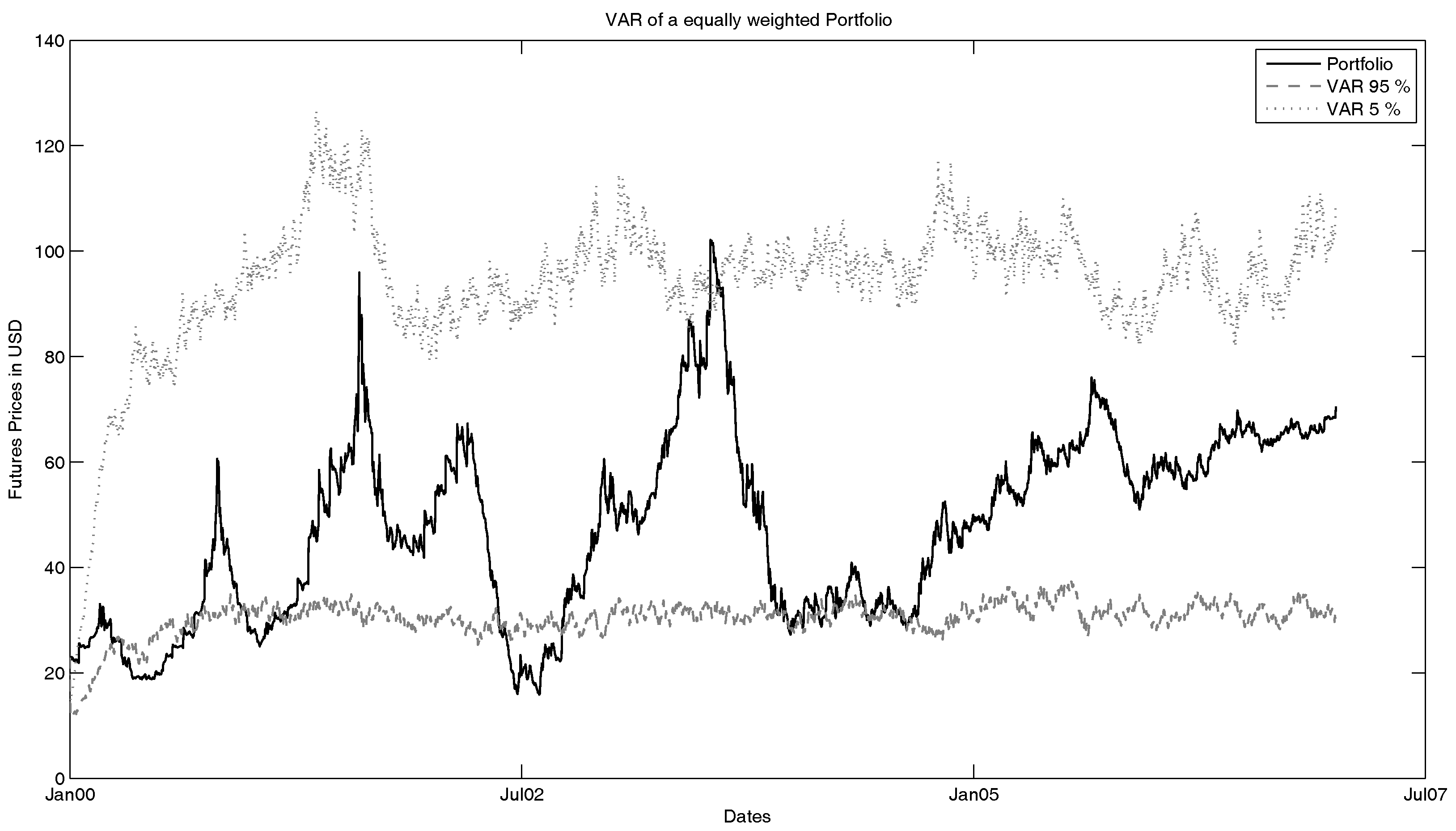
The value-at-risk we want to analyse is the 95%- and 5%-VaR of a portfolio consisting of all five observed ICE U.K. Natural Gas Futures with equal weights. The estimated VaR is shown in Figure 12. Here, one can see several facts and influences of the model. First, one should notice that the 95%-VaR is basically only the fitted seasonality function. This can be explained by the nature of the model. Since this model is based on a geometric model, all simulated time series have to be non-negative. Since we observe this on a time frame of ten years with much volatility, this means that with a high possibility, the simulated futures can have a low price, which is close to zero. Hence, the future price (without seasonality) becomes negligible compared to the seasonality function. When we take a look at the basic model (see Figure 13), we see that in this case, the future price is not as small as in case of the full model. This is explainable by the fact that we look at a Markov switching framework in the extended model. Hence, we have the possibility (compared to the parameters of the fitted Markov transition matrix) that one or more of the simulated time series are in the low variance state. This leads to smaller prices. Furthermore, due to negative jumps that can happen with a positive probability, the prices can be low in extreme cases.
Furthermore, we can notice that in the comparison, the 5%-VaR is underestimated in the full model. One percent of the real portfolio in the basic model lies above the 5%-VaR, compared to 10% outliers in the complete model. The 95%-VaR is overestimated by the basic model (basic model: 19% outliers; complete model: 0% outliers). An explanation for this can be found in the lack of jumps. As we have seen in the data analysis, we can observe jumps in the futures prices. These jumps are not reflected in the basic model (without seasonality, jumps and Markov switching), leading to a lower volatility of the VaR.
Secondly, we can see that the 5%-VaR shows reasonable results. By the logic of 5%-VaR, about 5% of the real portfolio should be above the simulated value-at-risk. Furthermore, one can see that the seasonality function highly influences the VaR, and if seasonality is not as strong as usual (no strong winter), the 5%-VaR is underestimated. This is also especially notable in the recovery phase of the financial crisis. One can observe here that the simulated VaR lies under the real portfolio. In this recovery phase, one can see that the portfolio development is not influenced by seasonality facts as strongly as at other times.
In Table 7, a comparison of the VaR is displayed for the basic model and the complete, full model for the whole time series (considering the timespan of 10 years). This reflects again the observations that we have made, when we analysed Figure 12 and Figure 13. We notice again that the 95%-VaR is underestimated by both models, respectively. Furthermore, the 5%-VaR of the complete model is much closer to the real 5%-VaR than the basic model.
Other fields of application could be the estimation of a spot price via an extrapolation of the simulated time series. Another application might be the pricing via this model. Nevertheless, we do not use risk-neutral valuation, which would be required, as this would be another field of research.
5. Conclusions
In this paper, we analysed the behaviour of natural gas futures prices. This led us to several effects that we want to consider in order to model such prices. We employed a cointegrated geometric model. Having calibrated the model, which was the first task of this paper, we then showed the value-at-risk calculation as one possible application of the model. We also used this application to compare the model to a basic version, in which we did not consider jumps, seasonality and a Markov switching framework.
There are several conclusions we can draw from the results of this research. First of all, one has to note the problems that emerge from the usage of such a model. The most severe problem is the calibration or the optimization, respectively. This problem arises from the matrix structure and the number of parameters calibrated on the one hand, and from the hidden risk factors, on the other hand. We solved this by using several optimization techniques and a Kalman filter.
Another problem is the possible over-fitting of the model by using a large amount of information for a low-dimensional number of risk factors. As we have seen, one has to be very careful with this issue, since, due to the form of the model, the simulated time series do not converge (in an empirical sense) if the parameter set is not chosen in the right way (see Section 3).
We have shown that it is useful to include cointegration and other aspects of commodities to fit standard measures of the real processes. Moreover, we included all state-of-the-art aspects of recent commodity models in our model. Furthermore, cointegration allows for more structure in our model. This has the advantage that the information is used in a more effective way, and less risk factors are needed. Nevertheless, this approach allows one to model the forward curve by simulating several points on a forward curve and interpolating them. This interpretation of cointegration can be used to describe several properties of a forward curve including backwardation or contango, which was not a central topic of this paper, but can be seen in the figures shown. For example, the futures curve switches from contango to backwardation, if the futures prices drop rapidly. The simulated paths with our models imitate this behaviour.
Compared to the existing models for commodity futures, we have taken several steps and approaches into consideration, which have not been part of other models. First, we used effects, such as seasonality and jumps, which are common for commodity models. Nevertheless, we used thinned-out compound Poisson processes to model these jumps, which was not used before in commodity models. We extended classical models by the use of cointegration in order to model the term structure of futures prices. Furthermore, we used a regime-switching approach to reproduce the volatility effects of commodity markets.
Since we considered futures prices for our calibration, a further step one can take from here is the evaluation of the spot prices via risk-neutral valuation or the valuation of other financial products (e.g., options) with such a risk-neutral measure. Furthermore, another next step could be the calibration via options on the commodity futures. This allows for a more precise calibration of the model due to the higher amount of information.
Acknowledgments
The authors gratefully acknowledge the comprehensive feed back of two anonymous referees which significantly improved this paper.
Author Contributions
The model shown was collaboratively developed by the three authors. Daniel Leonhardt conducted the data analysis and modelling (coding). Antony Ware and Rudi Zagst gave critical input. Antony Ware and Rudi Zagst reviewed and interpreted the results. The article was written as a shared effort.
Conflicts of Interest
The authors declare no conflict of interest.
References
- Adams, Zeno, and Thorsten Glück. 2015. Financialization in commodity markets: A passing trend or the new normal? Journal of Banking & Finance 60: 93–111. [Google Scholar] [CrossRef]
- Andersen, Leif. 2010. Markov models for commodity futures: Theory and practice. Quantitative Finance 10: 831–54. [Google Scholar] [CrossRef]
- Barndorff-Nielsen, Ole E., Fred Espen Benth, and Almut E. D. Veraart. 2015. Cross-Commodity Modelling by Multivariate Ambit Fields. In Commodities, Energy and Environmental Finance. Edited by René Aïd, Michael Ludkovski and Ronnie Sircar. Fields Institute Communications. New York: Springer, vol. 74, pp. 109–48. ISBN 978-1-4939-2732-6. [Google Scholar]
- Batchelor, Roy A, Amir H Alizadeh, and Ilias D Visvikis. 2007. Forecasting spot and forward prices in the international freight market. International Journal of Forecasting 23: 101–14. [Google Scholar] [CrossRef]
- Benth, Fred Espen, Jūratė Šaltytė Benth, and Steen Koekebakker. 2008. Stochastic Modeling of Electricity and Related Markets. Singapore: World Scientific Publishing, ISBN 978-981-281-230-8. [Google Scholar]
- Benth, Fred Espen, and Steen Koekebakker. 2015. Pricing of forwards and other derivatives in cointegrated commodity markets. Energy Economics 52: 104–17. [Google Scholar] [CrossRef] [Green Version]
- Benth, Fred Espen, and Paul Krühner. 2015. Derivatives pricing in energy markets: An infinite dimensional approach. SIAM Journal on Financial Mathematics 6: 825–69. [Google Scholar] [CrossRef]
- Brockwell, Peter J., and Richard A. Davis. 2002. Introduction to Time Series and Forecasting, 2nd ed. New York: Springer, ISBN 978-0-387-21657-7. [Google Scholar]
- Brunnermeier, Markus K., and Lasse Heje Pedersen. 2009. Market Liquidity and Funding Liquidity. Review of Financial Studies, Oxford University Press for Society for Financial Studies 22: 2201–38. [Google Scholar] [CrossRef]
- Carmona, Rene. 2015. Financialization of the Commodities Markets: A Non-Technical Introduction. New York: Springer, ISBN 978-1-4939-2732-6. [Google Scholar]
- Cartea, Avaro, and Thomas Williams. 2008. UK Gas Markets: The Market Price of Risk and Applications to Multiple Interruptible Supply Contracts. Energy Economics 30: 829–46. [Google Scholar] [CrossRef] [Green Version]
- Casassus, Jaime, and Pierre Collin-Dufrense. 2005. Stochastic convenience yield implied from commodity futures and interest rates. Review of Financial Studies 22: 2201–38. [Google Scholar] [CrossRef]
- Chowdhury, Abdur R. 2006. Futures market efficiency: Evidence from cointegration tests. Journal of Futures Markets 11: 577–89. [Google Scholar] [CrossRef]
- Daskalaki, Charoula, Alexandros Kostakis, and George S. Skiadopoulos. 2014. Are there common factors in individual commodity futures returns? Journal of Banking and Finance 40: 346–63. [Google Scholar] [CrossRef]
- Döttling, Rainer, and Pascal Heider. 2014. Spread volatility of cointegrated commodity pairs. The Journal of Energy Markets 6: 69–89. [Google Scholar] [CrossRef]
- Engle, Robert F., and Clive W. J. Granger. 1987. Co-Integration and Error Correction: Representation, Estimation, and Testing. Econometrica 55: 251–76. [Google Scholar] [CrossRef]
- Farkas, Walter, Elise Gourier, Robert Huitema, and Ciprian Necula. 2017. A Two-Factor Cointegrated Commodity Price Model with an Application to Spread Option Pricing. Journal of Banking & Finance 77: 249–68. [Google Scholar] [CrossRef]
- Geman, Hélyette. 2009. Commodities and Commodity Derivatives: Modeling and Pricing for Agriculturals, Metals and Energy. New York: John Wiley & Sons, ISBN 978-0-470-01218-5. [Google Scholar]
- Johansen, Søren. 1991. Estimation and hypothesis testing of cointegration vectors in Gaussian vector autoregressive models. Econometrica 59: 1551–80. [Google Scholar] [CrossRef]
- Karatzas, Ioannis, and Steven E. Shreve. 1991. Brownian Motion and Stochastic Calculus, 2nd ed. New York: Springer, ISBN 978-0-3879-6535-2. [Google Scholar]
- Kavoussanos, Manolis, Ilias Visvikis, and Dimitris Dimitrakopoulos. 2015. Economic spillovers between related derivative markets: The case of commodity and freight markets. Transportation Research Part E 68: 79–102. [Google Scholar] [CrossRef]
- Meyer-Brandis, Thilo, and Michael Morgan. 2014. A Dynamic Lévy Copula Model for the Spark Spread. In Quantitative Energy Finance. Edited by Peter Laurence, Valery A. Kholodnyi and Fred Espen Benth. New York: Springer, pp. 237–57. ISBN 978-1-4614-7247-6. [Google Scholar]
- Nielsen, Martin J., and E. S. Schwartz. 2004. Theory of storage and the pricing of commodity claims. Review of Derivatives Research 7: 5–24. [Google Scholar] [CrossRef]
- Panagiotidis, Theodore, and Emilie Rutledge. 2007. Oil and gas markets in the UK: Evidence from a cointegrating approach. Energy Economics 29: 239–347. [Google Scholar] [CrossRef]
- Paschke, Raphael, and Marcel Prokopczuk. 2009. Integrating multiple commodities in a model of stochastic price dynamics. Journal of Energy Markets 2: 47–82. [Google Scholar] [CrossRef]
- Petris, Giovanni, Sonia Petrone, and Patrizia Campagnoli. 2007. Dynamic Linear Models with R. New York: Springer, ISBN 978-0-387-77238-7. [Google Scholar]
- Pilipović, Dragana. 2007. Energy Risk: Valuing and Managing Energy Derivatives, 2nd ed. New York: McGraw-Hill, ISBN 978-0071485944. [Google Scholar]
- Silvennoinen, Annastiina, and S. Thorp. 2013. Financialization, crisis and commodity correlation dynamics. Journal of International Financial Markets, Institutions and Money 24: 42–65. [Google Scholar] [CrossRef]
- Schwartz, Eduardo. 1997. The stochastic behavior of commodity prices: Implications for valuation and hedging. Journal of Finance 52: 637–54. [Google Scholar] [CrossRef]
- Schwartz, Eduardo, and James E. Smith. 2000. Short-term variations and long-term dynamics in commodity prices. Management Science 46: 893–911. [Google Scholar] [CrossRef]
- Zhang, Chuanguo, and Xuqin Qu. 2015. The effect of global oil price shocks on China’s agricultural commodities. Energy Economics 51: 354–64. [Google Scholar] [CrossRef]
| 1. | Since the model includes a mean-reversion approach where all risk factors are interconnected via linear transformation, these effects can be observed within simulated time series of futures prices, e.g., if the prices radically drop, the futures go from normal backwardation to contango. |
| 2. | For a given time horizon and a fixed confidence level , the value-at-risk of the prices F represents the price that is not exceeded during the considered period of time with the specified probability . |
| 3. | This is, e.g., not the case if the amount of input data is too small or too large. In these cases, all simulated paths diverge instantly within 100–500 simulated days. |
Figure 1.
Prices of the ICE U.K. Natural Gas Futures with different maturities.
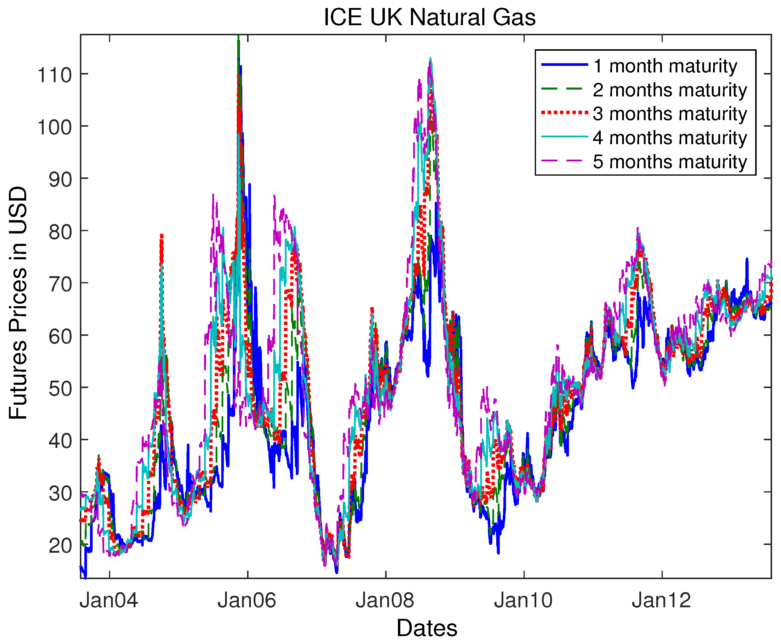
Figure 2.
ICE U.K. Natural Gas Futures log-prices and deseasonalized log-prices for the one-month rolling future.
Figure 2.
ICE U.K. Natural Gas Futures log-prices and deseasonalized log-prices for the one-month rolling future.
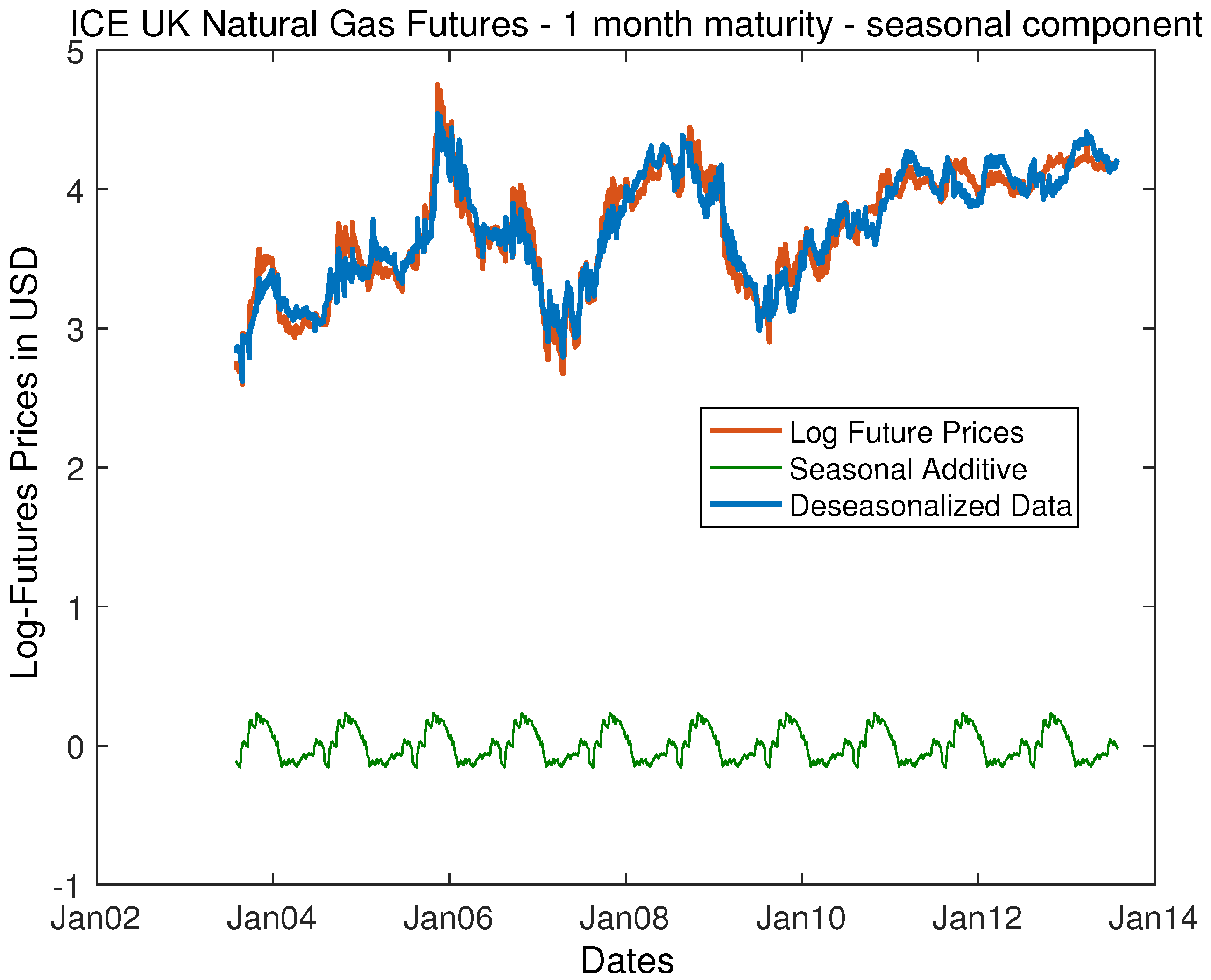
Figure 3.
ICE U.K. Natural Gas Futures: seasonal additive shown for one year for the one-month rolling future.
Figure 3.
ICE U.K. Natural Gas Futures: seasonal additive shown for one year for the one-month rolling future.
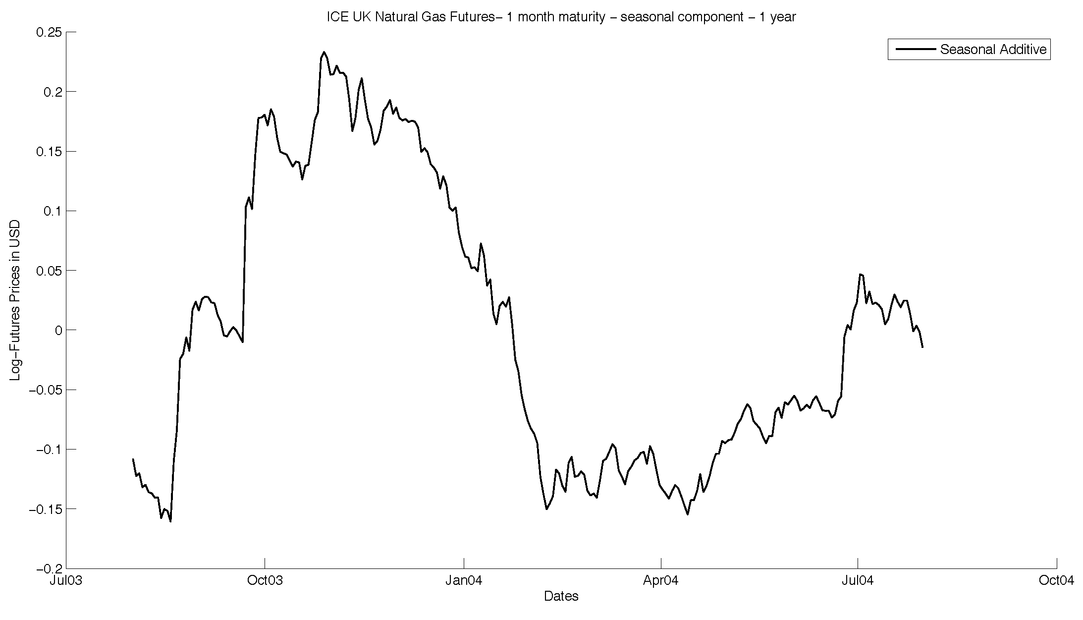
Figure 4.
ICE U.K. Natural Gas deseasonalized log-returns.

Figure 5.
Fitted Markov chain.

Figure 6.
Fitted Markov chain: one-year view.

Figure 7.
Histogram of the number of jumps occurring in a five-day window.

Figure 8.
Jumps for the different states.

Figure 9.
Box plots of the mean of simulated time series.

Figure 10.
Box plots of the standard deviation of simulated time series.
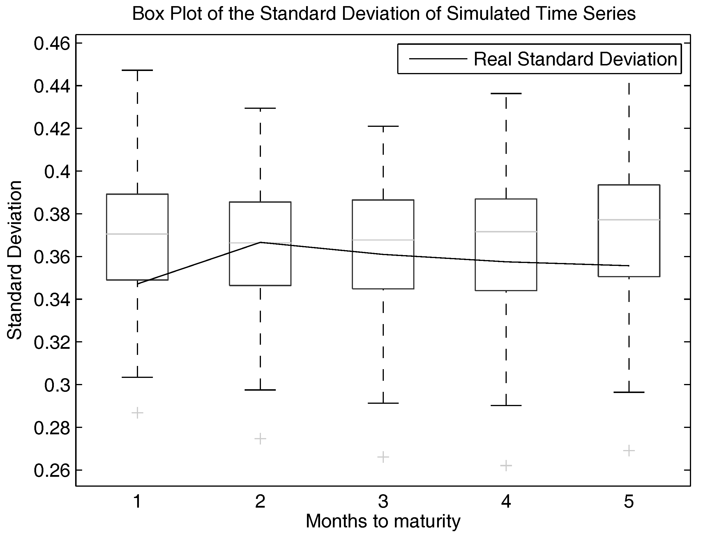
Figure 11.
Box plots of the skewness of simulated time series.
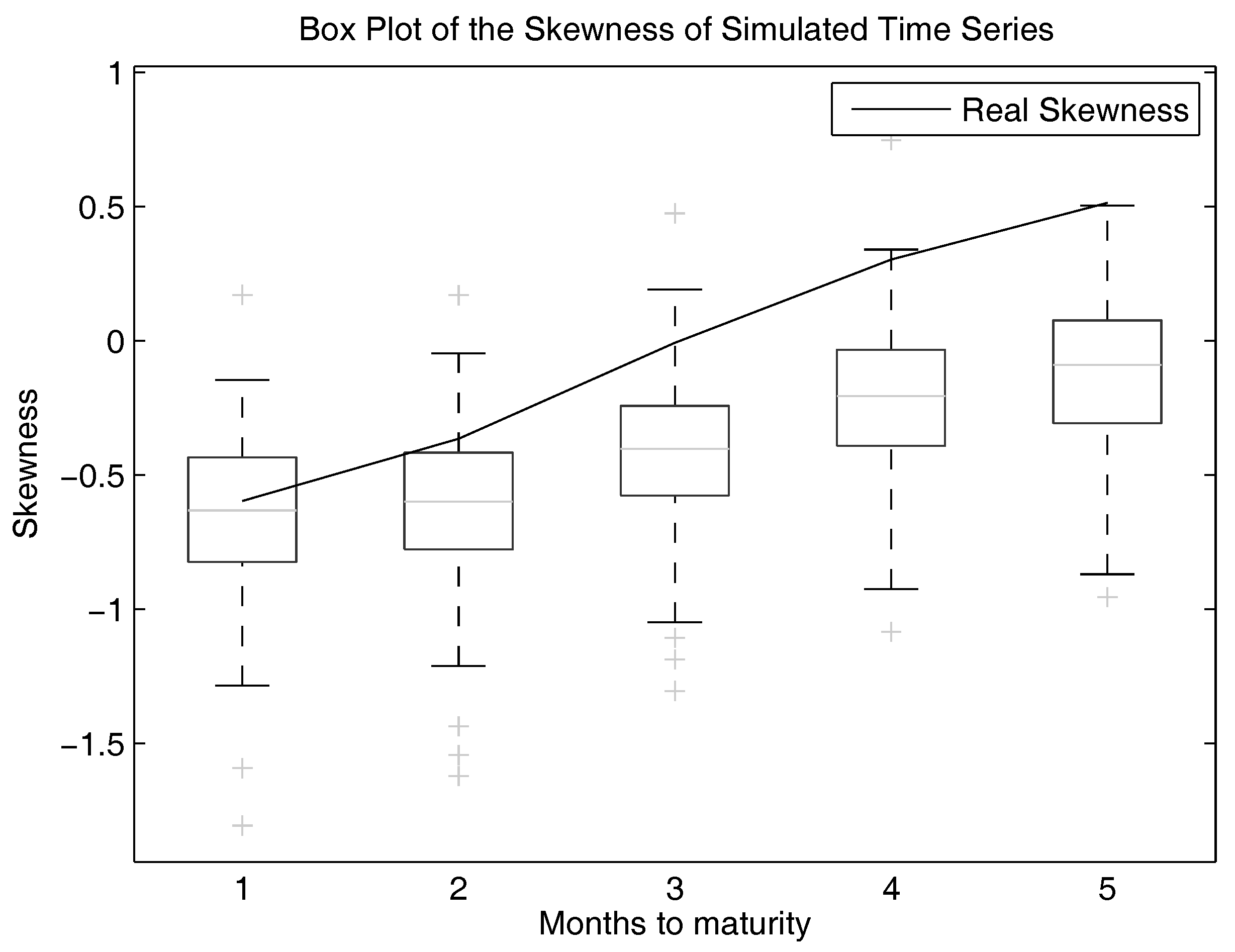
Figure 12.
VaR for the ICE U.K. Natural Gas Futures estimated with the extended geometric model.
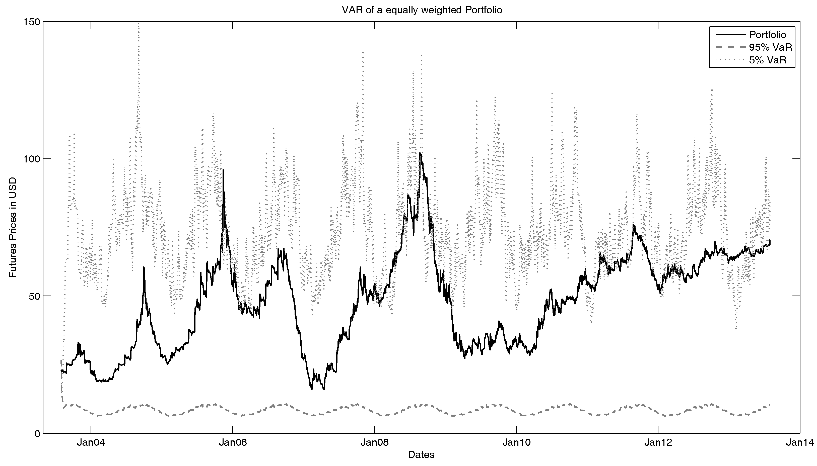
Figure 13.
VaR for the ICE U.K. Natural Gas Futures estimated with the basic, but still cointegrated geometric model.
Figure 13.
VaR for the ICE U.K. Natural Gas Futures estimated with the basic, but still cointegrated geometric model.


Table 1.
Correlation matrix of the ICE U.K. Natural Gas Futures prices with maturities from 1–5 months.
Table 1.
Correlation matrix of the ICE U.K. Natural Gas Futures prices with maturities from 1–5 months.
| Correlation | FN1 | FN2 | FN3 | FN4 | FN5 |
|---|---|---|---|---|---|
| FN1 | 1.0 | 0.96 | 0.87 | 0.77 | 0.65 |
| FN2 | 0.96 | 1.0 | 0.96 | 0.87 | 0.74 |
| FN3 | 0.87 | 0.96 | 1.0 | 0.96 | 0.84 |
| FN4 | 0.77 | 0.87 | 0.96 | 1.0 | 0.95 |
| FN5 | 0.65 | 0.74 | 0.84 | 0.95 | 1.0 |
Table 2.
Johansen trace test with a significance level of 0.05.
| r | H(r) | Stat | cValue | pValue | eigVal |
|---|---|---|---|---|---|
| 0 | 1 | 437.7947 | 76.9721 | 0.0010 | 0.0603 |
| 1 | 1 | 278.5820 | 54.0779 | 0.0010 | 0.0508 |
| 2 | 1 | 145.2208 | 35.1929 | 0.0010 | 0.0303 |
| 3 | 1 | 66.4185 | 20.2619 | 0.0010 | 0.0230 |
| 4 | 0 | 6.9356 | 9.1644 | 0.1302 | 0.0027 |
Table 3.
Markov transition matrix: probabilities to switch from a low volatility state to a high volatility state and vice versa.
Table 3.
Markov transition matrix: probabilities to switch from a low volatility state to a high volatility state and vice versa.
| Parameter | Estimate | Standard Deviation |
|---|---|---|
| 0.985 | 0.0008 | |
| 0.015 | 0.000 | |
| 0.0337 | 0.000 | |
| 0.9663 | 0.004 |
Table 4.
ICE U.K. futures: parameters of the underlying risk factors.
| FN1 | FN2 | FN3 | FN4 | FN5 | |||||||
| 0.6710 | 0.4914 | 0.3905 | 0.3722 | 0.3148 | −0.0005 | 0.0038 | −0.0085 | 0.0016 | |||
| 0.2167 | 0.2068 | 0.3304 | 0.3051 | 0.1403 | −0.0013 | −0.0077 | 0.0149 | −0.0021 | |||
| 1.4527 | 1.6972 | 1.7209 | 1.8546 | 2.018 | 0.0011 | −0.0034 | −0.0028 | 0.0113 | |||
| FN1 | FN2 | FN3 | FN4 | FN5 | |||||||
| 1.7255 | 1.3161 | 1.2062 | 1.0743 | 0.7731 | −0.0179 | −0.0061 | −0.0043 | 0.0238 | |||
| 0.5669 | 0.9917 | 0.8769 | 0.7518 | 0.9165 | 0.0007 | −0.0497 | −0.0344 | 0.1075 | |||
| 0.3179 | 0.3976 | 0.6491 | 0.9112 | 1.0649 | 0.0111 | 0.0047 | −0.006 | 0.0082 |
Table 5.
ICE U.K. futures: parameters of the diagonal correlation matrices.
| 0.0000 | 0.0010 | ||
| 0.0071 | 0.0010 | ||
| 0.0000 | 0.0010 | ||
| 0.0022 | 0.0010 | ||
| 0.0000 | 0.0010 | ||
| 0.0010 | 0.0016 | ||
| 0.0020 | 0.0019 | ||
| 0.0002 | 0.0001 |
Table 6.
ICE U.K. Natural Gas Futures: parameters of the thinned-out Poisson process.
| 19.5534 | |||||
| −0.0120 | 0.0628 | 0.0485 | |||
| 0.0045 | 0.1199 | 0.1748 | |||
| 0.0068 | 0.1223 | 0.2524 | |||
| 0.0285 | 0.1445 | 0.2039 | |||
| −0.0017 | 0.1187 | 0.3204 | |||
| ∞ | |||||
| 0 | 0 | ||||
| 0 | 0 | ||||
| 0 | 0 | ||||
| 0 | 0 | ||||
| 0 | 0 | ||||
| 12.3864 | |||||
| 0.2167 | 0.1622 | 0.2500 | |||
| 0.2333 | 0.0527 | 0.2045 | |||
| 0.1195 | 0.1541 | 0.2273 | |||
| 0.0510 | 0.3002 | 0.1364 | |||
| −0.0210 | 0.2570 | 0.1818 | |||
| 272.5000 | |||||
| 0.2668 | 0.0387 | ||||
| 0.3340 | 0.0897 | ||||
| 0.3255 | 0.1848 | ||||
| 0.3336 | 0.1797 | ||||
| 0.3480 | 0.1611 | ||||
Table 7.
VaR of the different models and the real ICE U.K. Futures data.
| Model/Data | 5%-VaR | %95-VaR |
|---|---|---|
| Data Set | 74.12 | 8.44 |
| Complete Model | 73.35 | 21.36 |
| Basic Model | 96.11 | 30.99 |
© 2017 by the authors. Licensee MDPI, Basel, Switzerland. This article is an open access article distributed under the terms and conditions of the Creative Commons Attribution (CC BY) license (http://creativecommons.org/licenses/by/4.0/).
Share and Cite
MDPI and ACS Style
Leonhardt, D.; Ware, A.; Zagst, R. A Cointegrated Regime-Switching Model Approach with Jumps Applied to Natural Gas Futures Prices. Risks 2017, 5, 48. https://doi.org/10.3390/risks5030048
AMA Style
Leonhardt D, Ware A, Zagst R. A Cointegrated Regime-Switching Model Approach with Jumps Applied to Natural Gas Futures Prices. Risks. 2017; 5(3):48. https://doi.org/10.3390/risks5030048
Chicago/Turabian StyleLeonhardt, Daniel, Antony Ware, and Rudi Zagst. 2017. "A Cointegrated Regime-Switching Model Approach with Jumps Applied to Natural Gas Futures Prices" Risks 5, no. 3: 48. https://doi.org/10.3390/risks5030048
Note that from the first issue of 2016, this journal uses article numbers instead of page numbers. See further details here.