Model Uncertainty in Operational Risk Modeling Due to Data Truncation: A Single Risk Case

Abstract

Over the last decade, researchers, practitioners, and regulators have had intense debates about how to treat the data collection threshold in operational risk modeling. Several approaches have been employed to fit the loss severity distribution: the empirical approach, the “naive” approach, the shifted approach, and the truncated approach. Since each approach is based on a different set of assumptions, different probability models emerge. Thus, model uncertainty arises. The main objective of this paper is to understand the impact of model uncertainty on the value-at-risk (VaR) estimators. To accomplish that, we take the bank’s perspective and study a single risk. Under this simplified scenario, we can solve the problem analytically (when the underlying distribution is exponential) and show that it uncovers similar patterns among VaR estimates to those based on the simulation approach (when data follow a Lomax distribution). We demonstrate that for a fixed probability distribution, the choice of the truncated approach yields the lowest VaR estimates, which may be viewed as beneficial to the bank, whilst the “naive” and shifted approaches lead to higher estimates of VaR. The advantages and disadvantages of each approach and the probability distributions under study are further investigated using a real data set for legal losses in a business unit (Cruz 2002).

1. Introduction

Basel II/III and Solvency II are the leading international regulatory frameworks for banking and insurance industries, and mandate that financial institutions build separate capital reserves for operational risk. Within the advanced measurement approach (AMA) framework, the loss distribution approach (LDA) is the most sophisticated tool for estimating the operational risk capital. According to LDA, the risk-based capital is an extreme quantile of the annual aggregate loss distribution (e.g., the 99.9th percentile), which is called value-at-risk or VaR. Some recent discussions between the industry and the regulatory community in the United States reveal that the LDA implementation still has a number of “thorny” issues (AMA Group 2013). One such issue is the treatment of data collection threshold. Here is what is stated on page 3 of the same document: “Although the industry generally accepts the existence of operational losses below the data collection threshold, the appropriate treatment of such losses in the context of capital estimation is still widely debated.”

Various assumptions about the data collection threshold have been considered in the existing literature: known threshold (Baud et al. 2002; Shevchenko and Temnov 2009), threshold as unknown parameter (Baud et al. 2002), stochastic threshold whose distribution has to be modeled (Baud et al. 2002; de Fontnouvelle et al. 2006), and time varying threshold that may scale according to inflation and business factors (Shevchenko and Temnov 2009). In this paper, we will assume that the threshold is known. Given (external) operational risk databases (which often collect losses exceeding, for example, $1 million), such an assumption is appropriate.

Further, the annual aggregate loss variable is a combination of two variables—loss frequency and loss severity—and there are different ways to estimate risk-based capital. One way is to estimate the untruncated severity and truncation-adjusted frequency and then compute VaR. This approach follows directly from the results described by Brazauskas, Jones, and Zitikis (Brazauskas et al. 2015). Another way is to estimate the truncated severity and unadjusted frequency to compute VaR. For a comprehensive review of analytic techniques for truncated data in the context of operational risk modeling, see Cruz, Peters, Shevchenko (Cruz et al. 2015, sct. 7.9). Furthermore, as is known in practice, the severity distribution is a key driver of the capital estimate (Opdyke 2014). This is the part of the aggregate model where initial assumptions about the data collection threshold are most influential. A number of authors have examined some aspects of this topic in the past (e.g., Cavallo et al. 2012; Chernobai et al. 2007; Ergashev et al. 2016; Luo et al. 2007; Moscadelli et al. 2005). The modeling approaches they (collectively) considered include: the empirical approach, the “naive” approach, the shifted approach, and the truncated approach. Since each approach is based on a different set of assumptions, different probability models emerge. Thus, model uncertainty arises.

The main objective of this paper is to understand the impact of model uncertainty on risk measurements, and (hopefully) help settle the debate about the treatment of data collection threshold in the context of capital estimation. Solving such a problem under a general setup (i.e., by considering many interdependent risks and multiple stakeholders) is only possible through extensive simulations, but that would not produce much insight. Therefore, we simplify the problem by taking the bank’s perspective and by studying a single risk. Under this simplified scenario, we can solve the problem analytically (when the underlying distribution is exponential), and show that it uncovers similar patterns among VaR estimates to those based on the simulation approach (when data follow a Lomax distribution). We demonstrate that for a fixed probability distribution, the choice of the truncated approach yields lowest VaR estimates, which may be viewed as beneficial to the bank, whilst the “naive” and shifted approaches lead to higher estimates of VaR. As for the choice of severity distributions, besides the Lomax distribution (which is heavy tailed and hence appropriate in operational risk modeling), we intentionally select the light-tailed exponential distribution to show what happens to VaR estimates when incorrect assumptions are made. Moreover, our step-by-step analysis not only shows “what happens” to VaR estimates, but it helps understand the questions of “how” and “why” it happens. Additionally, perhaps surprisingly, our numerical illustrations reveal why the shifted approach is still popular. That is because it is flexible enough to pass standard model validation tests and thus cannot be discarded from practical use based on such tools alone. In summary, this paper contributes to the existing literature by performing an extensive investigation of the impact that model uncertainty has on the VaR estimators, justifies the soundness of the regulatory recommendation (i.e., use the truncated approach), and paves the way for a number of research problems in this important area.

It is worth noting here that the model uncertainty considered in this paper is an epistemic one, not a random uncertainty. It can be reduced—but not completely eliminated—by employing sound model validation tools, and in some cases (e.g., when the shifted approach is used) may require out-of-model knowledge. In a more general context, model uncertainty is an important topic within the model risk governance framework as regulated by the OCC and the Federal Reserve Bank in the U.S. and the Basel Committee on Banking Supervision for the G20 countries (e.g., Basel Coordination Committee 2014; Office of the Comptroller of the Currency 2011).

The rest of the paper is structured as follows. In Section 2, we describe how model uncertainty emerges and study its effects on VaR estimates. This is done by employing theoretical results (presented in Appendix A) and via Monte Carlo simulations. Next, in Section 3, these explorations are further illustrated using a real data set for legal losses in a business unit. Finally, concluding remarks are offered in Section 4. Additionally, in Appendix A we provide some technical tools that are essential for analytic treatment of the problem. In particular, key probabilistic features of the generalized Pareto distribution are presented, and several asymptotic theorems of mathematical statistics are specified.

2. Model Uncertainty

We start this section by introducing the problem and describing how model uncertainty arises. Then, in Section 2.2, we review several typical models used for estimating VaR. Finally, using the theoretical results of Appendix and Monte Carlo simulations, we finish with two parametric examples, where we evaluate the probability of overestimating true VaR for exponential and Lomax distributions.

2.1. Motivation

In order to fully understand the problem, in this paper we will walk the reader through the entire modeling process and demonstrate how our assumptions affect the end product, which is the estimate of severity VaR. Since the problem involves collected data, initial assumptions, and statistical inference (in this case, point estimation and assessment of estimates’ variability), it will be tackled with statistical tools, including theoretical tools (asymptotics), Monte Carlo simulations, and real-data case studies. Let us briefly discuss data, assumptions, and inference. As noted in Section 1, it is generally agreed that operational losses exist above and below the data collection threshold. Therefore, this implies that choosing a modeling approach is equivalent to deciding on how much probability mass there is below the threshold.

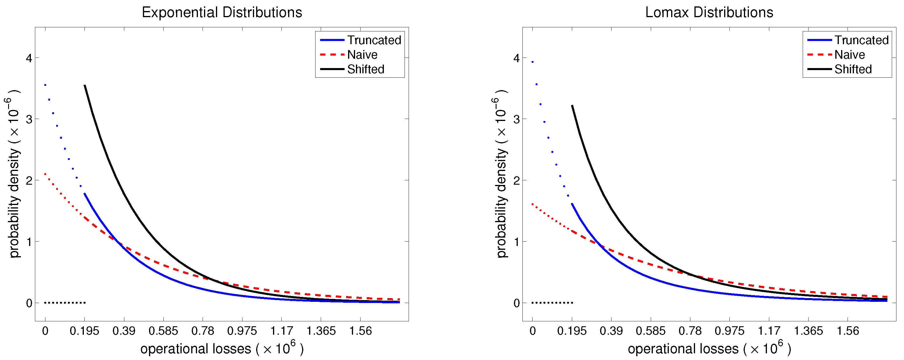
In Figure 1, we provide graphs of truncated, naive, and shifted probability density functions of two distributions (studied formally in Section 2.3): Exponential, which is a light-tailed model; and Lomax, with the tail parameter $\alpha =3.5$, which is a moderately-tailed model (it has three finite moments). We clearly see that those models are quite different below the threshold $t=195,000$, but in practice that would be unobserved. On the other hand, in the observable range (i.e., above $t=195,000$), the plotted density functions are similar (note that the vertical axes are in very small units, ${10}^{-6}$) and converge to each other as losses get larger (note how little differentiation there is among the curves when losses exceed 1,000,000). Moreover, it is even difficult to spot a difference between the corresponding exponential and Lomax models, though the two distributions possess distinct theoretical properties (e.g., for one all moments are finite, whereas for the other only three are). Additionally, since probability mass below the threshold is one of the “known unknowns,” it will have to be estimated from the observed data (above t). As will be shown in the case study of Section 3, this task may look straightforward, but its outcomes vary and are heavily influenced by the initial assumptions.

To formalize this dicussion, suppose that $Y_1,\dots ,Y_N$ represent (positive and i.i.d.) loss severities resulting from operational risk, and let us denote their probability density function (pdf), cumulative distribution function (cdf), and quantile function (qf) as f, F, and $F^{-1}$, respectively. Then, the problem of estimating VaR-based capital is equivalent to finding an estimate of qf at some probability level (e.g., $F^{-1}\left(\beta \right)$). The difficulty here is that we observe only those $Y_i$’s that exceed some known data collection threshold $t\gg 0$. That is, the actually observed variables are $X_i$’s with

$$X_1\stackrel{d}{=}{Y}_{i_1}|Y_{i_1}>t,\dots ,X_n\stackrel{d}{=}{Y}_{i_n}|Y_{i_n}>t,$$

(1)

where $\stackrel{d}{=}$ denotes “equal in probability” and $n={\sum }_{j=1}^N\mathbf{1}\left\{Y_j>t\right\}$. Their cdf $F_{*}$, pdf $f_{*}$, qf $F_{*}^{-1}$ are related to F, f, $F^{-1}$, and given by

$$F_{*}\left(x\right)=\frac{F\left(x\right)-F\left(t\right)}{1-F\left(t\right)},f_{*}\left(x\right)=\frac{f\left(x\right)}{1-F\left(t\right)},F_{*}^{-1}\left(u\right)=F^{-1}\left(u+(1-u)F\left(t\right)\right)$$

(2)

for $x\ge t$ and $0<u<1$, and for $x<t$, $f_{*}\left(x\right)=F_{*}\left(x\right)=0$.

Further, let us investigate the behavior of $F_{*}^{-1}\left(u\right)$ from a purely mathematical point of view. Since the qf of continuous random variables (which is the case for loss severities) is a strictly increasing function and $(1-u)F\left(t\right)\ge 0$, it follows that

$$F_{*}^{-1}\left(u\right)=F^{-1}\left(u+(1-u)F\left(t\right)\right)\ge F^{-1}\left(u\right),0<u<1,$$

with the inequality being strict unless $F\left(t\right)=0$. This implies that any quantile of the observable variable X is never below the corresponding quantile of the unobservable variable Y, which is true VaR. This fact is certainly not new (for example, see the extensive analysis by Opdyke (2014), about the effect of Jensen’s inequality in VaR estimation). However, if we now change our perspective from mathematical to statistical and take into account the method of how VaR is estimated, we could augment the above discussion with new insights and improve our understanding.

A review of existing methods shows that, besides estimation of VaR using Equations (1) and (2) under the truncated distribution framework, there are other parametric methods that employ different strategies, such as the naive and shifted approaches (described in Section 2.2.2). In particular, those two approaches use the data $X_1,\dots ,X_n$ and either ignore t or recognize it in some other way than Equation (2). Thus, model uncertainty emerges.

2.2. Typical Models

2.2.1. Empirical Model

As mentioned earlier, the empirical model is restricted to the range of observed data. So, it uses data from Equation (1), but since the empirical estimator $\widehat{F}\left(t\right)=0$, Formulas (2) simplify to ${\widehat{F}}_{*}\left(x\right)=\widehat{F}\left(x\right)$, ${\widehat{f}}_{*}\left(x\right)=\widehat{f}\left(x\right)$, for $x\ge t$, and ${\widehat{F}}_{*}^{-1}\left(u\right)={\widehat{F}}^{-1}\left(u\right)$. Thus, the model cannot take full advantage of Equation (2). In this case, the VaR($\beta$) estimator is simply ${\widehat{F}}^{-1}\left(\beta \right)=X_{(\lceil n\beta \rceil )}$, and as follows from Theorem A1,

$$X_{(\lceil n\beta \rceil )}is\mathcal{AN}\left(F_{*}^{-1}\left(\beta \right),\frac{1}{n}\frac{\beta (1-\beta )}{f_{*}^2\left(F_{*}^{-1}\left(\beta \right)\right)}\right).$$

We now can evaluate the probability of overestimating the true VaR by a certain percentage; i.e., we want to study function $H\left(c\right):=\mathbf{P}\left\{X_{(\lceil n\beta \rceil )}>c{F}^{-1}\left(\beta \right)\right\}$ for $c\ge 1$. Using Z to denote the standard normal random variable and $\Phi$ for its cdf, and taking into account Equation (2), we proceed as follows:

$$\begin{array}{cc}\hfill H\left(c\right)& =\mathbf{P}\left\{X_{(\lceil n\beta \rceil )}>c{F}^{-1}\left(\beta \right)\right\}\approx \mathbf{P}\left\{Z>\left[c{F}^{-1}\left(\beta \right)-F_{*}^{-1}\left(\beta \right)\right]\times {\left(\frac{1}{n}\frac{\beta (1-\beta )}{f_{*}^2\left(F_{*}^{-1}\left(\beta \right)\right)}\right)}^{-1/2}\right\}\hfill \\ & =1-\Phi \left(\sqrt{\frac{n}{\beta (1-\beta )}}\left[c{F}^{-1}\left(\beta \right)-F^{-1}(\beta +(1-\beta )F\left(t\right))\right]\times \frac{f\left(F^{-1}(\beta +(1-\beta )F\left(t\right))\right)}{1-F\left(t\right)}\right).\hfill \end{array}$$

From this formula, we clearly see that $0.50\le H\left(1\right)<1$, with the lower bound being achieved when $F\left(t\right)=0$. Additionally, at the other extreme, when $c\to \infty$, we observe $H\left(c\right)\to 0$. Additional numerical illustrations are provided in

Table 1. Function $H\left(c\right)$ evaluated for various combinations of c, confidence level $\beta$, proportion of unobserved data $F\left(t\right)$, and severity distributions with varying degrees of tail heaviness ranging from light- and moderate-tailed to heavy-tailed. The sample size is $n=100$.

c	$\mathit{\beta }$	$\mathit{F}\left(\mathit{t}\right)=0$			$\mathit{F}\left(\mathit{t}\right)=0.5$			$\mathit{F}\left(\mathit{t}\right)=0.9$
		Light	Moderate	Heavy	Light	Moderate	Heavy	Light	Moderate	Heavy
1	0.95	0.500	0.500	0.500	0.944	0.925	0.874	1.000	1.000	0.981
	0.995	0.500	0.500	0.500	0.688	0.672	0.638	0.949	0.884	0.738
	0.999	0.500	0.500	0.500	0.587	0.579	0.563	0.767	0.703	0.612
1.2	0.95	0.085	0.178	0.331	0.585	0.753	0.824	1.000	1.000	0.978
	0.995	0.226	0.349	0.444	0.398	0.551	0.612	0.811	0.840	0.734
	0.999	0.331	0.424	0.475	0.414	0.517	0.550	0.615	0.668	0.610
1.5	0.95	0.000	0.010	0.138	0.032	0.326	0.726	0.968	0.996	0.975
	0.995	0.030	0.167	0.362	0.083	0.364	0.571	0.403	0.756	0.727
	0.999	0.137	0.317	0.437	0.191	0.424	0.532	0.358	0.613	0.606
2	0.95	0.000	0.000	0.015	0.000	0.009	0.523	0.056	0.930	0.968
	0.995	0.000	0.026	0.240	0.001	0.127	0.501	0.017	0.577	0.715
	0.999	0.014	0.170	0.376	0.025	0.280	0.500	0.073	0.516	0.600

Threshold t is 0 for $F\left(t\right)=0$ and $195,000$ for $F\left(t\right)=0.5,0.9$. Distributions: $Light=\mathrm{exponential}\left(\sigma \right)$, $Moderate=\mathrm{Lomax}(\alpha =3.5,{\theta }_1)$, $Heavy=\mathrm{Lomax}(\alpha =1,{\theta }_2)$. For $F\left(t\right)=0$: $\sigma ={\theta }_1={\theta }_2=1$. For $F\left(t\right)=0.5$: $\sigma =281,326$, ${\theta }_1=890,355$, ${\theta }_2=195,000$. For $F\left(t\right)=0.9$: $\sigma =84,687$, ${\theta }_1=209,520$, ${\theta }_2=21,667$.

.

Several conclusions emerge from the table. First, the case $F\left(t\right)=0$ is a benchmark case that illustrates the behavior of the empirical estimator when data is completely observed (and in that case $X_{(\lceil n\beta \rceil )}$ would be a consistent method for estimating $\mathrm{VaR}\left(\beta \right)$). We see that $H\left(1\right)=0.5$, and then it quickly decreases to 0 as c increases. The decrease is quickest for the light-tailed distribution, exponential$(\sigma =1)$, and slowest for the heavy-tailed Lomax $(\alpha =1,{\theta }_2=1)$, which has no finite moments. Second, as less data is observed (i.e., as $F\left(t\right)$ increases to 0.5 and 0.9), the probability of overestimating true VaR increases for all types of distribution. For example, while the probability of overestimating $\mathrm{VaR}\left(0.995\right)$ by 20% ($c=1.2$) for the light-tailed distribution is only 0.226 for $F\left(t\right)=0$, it increases to 0.398 and 0.811 for $F\left(t\right)=0.5$ and $0.9$, respectively. If severity follows the heavy-tailed distribution, then $H\left(1.2\right)$ is 0.444, 0.612, 0.734 for $F\left(t\right)=0,0.5,0.9$, respectively. Finally, in practice, typical scenarios would be near $F\left(t\right)=0.9$ with moderate- or heavy-tailed severity distributions, which corresponds to quite unfavorable patterns in the table. Indeed, function $H\left(c\right)$ declines very slowly, and the probability of overestimating $\mathrm{VaR}\left(0.995\right)$ by 100% seems like a norm (0.577 and 0.715).

2.2.2. Parametric Models

We discuss three parametric approaches: truncated, naive, and shifted.

Truncated Approach: The truncated approach uses the observed data $X_1,\dots ,X_n$ and fully recognizes its distributional properties. That is, it takes into account Equation (2) and derives maximum likelihood estimator (MLE) values by maximizing the following log-likelihood function:

$$log{\mathcal{L}}_T\left({\theta }_1,\dots ,{\theta }_k|X_1,\dots ,X_n\right)=\sum _{i=1}^{n}log{f}_{*}\left(X_i\right)=\sum _{i=1}^{n}log\left(\frac{f\left(X_i\right)}{1-F\left(t\right)}\right),$$

(3)

where ${\theta }_1,\dots ,{\theta }_k$ are the parameters of pdf f. Once parameter MLEs are available, $\mathrm{VaR}\left(\beta \right)$ estimate is found by plugging those MLE values into $F^{-1}\left(\beta \right)$.                                            □

Naive Approach: The naive approach uses the observed data $X_1,\dots ,X_n$, but ignores the presence of threshold t. That is, it bypasses Equation (2) and derives MLE values by maximizing the following log-likelihood function:

$$log{\mathcal{L}}_N\left({\theta }_1,\dots ,{\theta }_k|X_1,\dots ,X_n\right)=\sum _{i=1}^{n}logf\left(X_i\right).$$

(4)

Notice that since $f\left(X_i\right)\le f\left(X_i\right)/[1-F\left(t\right)]=f_{*}\left(X_i\right)$, with the inequality being strict for $F\left(t\right)>0$, the log-likelihood of the naive approach will always be less than that of the truncated approach. This in turn implies that parameter MLEs of pdf f derived using the naive approach will always be suboptimal, unless $F\left(t\right)=0$. Finally, $\mathrm{VaR}\left(\beta \right)$ estimate is computed by inserting parameter MLEs (the ones found using the naive approach) into $F^{-1}\left(\beta \right)$.                                            □

Shifted Approach: The shifted approach uses the observed data $X_1,\dots ,X_n$ and recognizes threshold t by first shifting the observations by t. Then, it derives parameter MLEs by maximizing the following log-likelihood function:

$$log{\mathcal{L}}_S\left({\theta }_1,\dots ,{\theta }_k|X_1,\dots ,X_n\right)=\sum _{i=1}^{n}logf(X_i-t).$$

(5)

By comparing Equations (4) and (5), we can easily see that the naive approach is a special case of the shifted approach (with $t=0$). Moreover, although this may only be of interest to theoreticians, one could introduce a class of shifted models by considering $f(X_i-s)$, with $0\le s\le t$, and create infinitely many versions of the shifted model. Finally, $\mathrm{VaR}\left(\beta \right)$ is estimated by applying parameter MLEs (the ones found using the shifted approach) to $F^{-1}\left(\beta \right)+t$.                                            □

2.3. Parametric VaR Estimation

2.3.1. Example 1: Exponential Distribution

Suppose $Y_1,\dots ,Y_N$ are i.i.d. and follow an exponential distribution, with pdf, cdf, and qf given by Equations (A1), (A2), and (A4), respectively, with $\gamma =0$ and $\mu =0$. However, we observe only variable X, whose relation to Y is governed by Equations (1) and (2). Now, by plugging exponential pdf and/or cdf into the log-likelihoods Equations (3)–(5), we obtain

$$\begin{array}{cc}\hfill log{\mathcal{L}}_T\left(\sigma |X_1,\dots ,X_n\right)& =\sum _{i=1}^{n}log\left(\frac{f\left(X_i\right)}{1-F\left(t\right)}\right)=\sum _{i=1}^{n}log\left(\frac{{\sigma }^{-1}{e}^{-X_i/\sigma }}{e^{-t/\sigma }}\right)\hfill \\ & =-nlog\sigma +\sum _{i=1}^n\frac{-(X_i-t)}{\sigma },\hfill \end{array}$$

(6)

$$\begin{array}{cc}\hfill log{\mathcal{L}}_N\left(\sigma |X_1,\dots ,X_n\right)& =\sum _{i=1}^{n}logf\left(X_i\right)=\sum _{i=1}^{n}log\left({\sigma }^{-1}{e}^{-X_i/\sigma }\right)\hfill \\ & =-nlog\sigma +\sum _{i=1}^n\frac{-X_i}{\sigma },\hfill \end{array}$$

(7)

$$\begin{array}{cc}\hfill log{\mathcal{L}}_S\left(\sigma |X_1,\dots ,X_n\right)& =\sum _{i=1}^{n}logf(X_i-t)=\sum _{i=1}^{n}log\left({\sigma }^{-1}{e}^{-(X_i-t)/\sigma }\right)\hfill \\ & =-nlog\sigma +\sum _{i=1}^n\frac{-(X_i-t)}{\sigma },\hfill \end{array}$$

(8)

where the subscripts $T,N,S$ (for $\mathcal{L}$) denote “truncated”, “naive”, and “shifted”, respectively. Then, by maximizing the log-likelihoods (6)–(8) with respect to $\sigma$, we get the following MLE formulas for parameter $\sigma$ under the truncated, naive, and shifted approaches:

$${\widehat{\sigma }}_T=\overline{X}-t,{\widehat{\sigma }}_N=\overline{X},{\widehat{\sigma }}_S=\overline{X}-t,$$

where $\overline{X}=n^{-1}{\sum }_{i=1}^n{X}_i$.

Next, by inserting ${\widehat{\sigma }}_T$, ${\widehat{\sigma }}_N$, and ${\widehat{\sigma }}_S$ into the corresponding qf’s as described in Section 2.2.2, we get the following $\mathrm{VaR}\left(\beta \right)$ estimators:

$${\widehat{\mathrm{VaR}}}_T\left(\beta \right)=-{\widehat{\sigma }}_{T}log(1-\beta ),{\widehat{\mathrm{VaR}}}_N\left(\beta \right)=-{\widehat{\sigma }}_{N}log(1-\beta ),{\widehat{\mathrm{VaR}}}_S\left(\beta \right)=-{\widehat{\sigma }}_{S}log(1-\beta )+t.$$

Further, a direct application of Theorem A2 for ${\widehat{\sigma }}_T$ (with obvious adjustment for ${\widehat{\sigma }}_N$), yields that

$${\widehat{\sigma }}_{T}is\mathcal{AN}\left(\sigma ,\frac{{\sigma }^2}{n}\right),{\widehat{\sigma }}_N\mathrm{is}\mathcal{AN}\left(\sigma +t,\frac{{\sigma }^2}{n}\right),{\widehat{\sigma }}_S\mathrm{is}\mathcal{AN}\left(\sigma ,\frac{{\sigma }^2}{n}\right).$$

Furthermore, having established $\mathcal{AN}$ for parameter MLEs, we can apply Theorem A3 and specify asymptotic distributions for VaR estimators. They are as follows:

$${\widehat{\mathrm{VaR}}}_T\left(\beta \right)\mathrm{is}\mathcal{AN}\left(-\sigma log(1-\beta ),\frac{{\sigma }^2{log}^2(1-\beta )}{n}\right),$$

$${\widehat{\mathrm{VaR}}}_N\left(\beta \right)\mathrm{is}\mathcal{AN}\left(-(\sigma +t)log(1-\beta ),\frac{{\sigma }^2{log}^2(1-\beta )}{n}\right),$$

$${\widehat{\mathrm{VaR}}}_S\left(\beta \right)\mathrm{is}\mathcal{AN}\left(-\sigma log(1-\beta )+t,\frac{{\sigma }^2{log}^2(1-\beta )}{n}\right).$$

Note that while all three estimators are equivalent in terms of the asymptotic variance, they are centered around different targets. The mean of the truncated estimator is the true quantile of the underlying exponential model (estimating which is the objective of this exercise) and the mean of the other two methods is shifted upwards; in both cases, the shift is a function of threshold t.

Finally, as was done for the empirical VaR estimator in Section 2.2.1, we now define function $H\left(c\right)=\mathbf{P}\left\{\widehat{\mathrm{VaR}}\left(\beta \right)>c{F}^{-1}\left(\beta \right)\right\}$ for $c\ge 1$, the probability of overestimating the target by $(c-1)100\%$ for each parametric VaR estimator and study its behavior:

$$H_T\left(c\right)\approx 1-\Phi \left((c-1)\sqrt{n}\right),H_N\left(c\right)\approx 1-\Phi \left((c-1)\sqrt{n}-\sqrt{n}(t/\sigma )\right),$$

$$H_S\left(c\right)\approx 1-\Phi \left((c-1)\sqrt{n}+\sqrt{n}(t/\sigma ){log}^{-1}(1-\beta )\right).$$

Table 2. Functions $H_T\left(c\right)$, $H_N\left(c\right)$, $H_S\left(c\right)$ evaluated for various combinations of c, confidence level $\beta$, and proportion of unobserved data $F\left(t\right)$. (The sample size is $n=100$.)

c	$\mathit{\beta }$	$\mathit{F}\left(\mathit{t}\right)=0$			$\mathit{F}\left(\mathit{t}\right)=0.5$			$\mathit{F}\left(\mathit{t}\right)=0.9$
		T	N	S	T	N	S	T	N	S
1	0.95	0.500	0.500	0.500	0.500	1.000	0.990	0.500	1.000	1.000
	0.995	0.500	0.500	0.500	0.500	1.000	0.905	0.500	1.000	1.000
	0.999	0.500	0.500	0.500	0.500	1.000	0.842	0.500	1.000	1.000
1.2	0.95	0.023	0.023	0.023	0.023	1.000	0.623	0.023	1.000	1.000
	0.995	0.023	0.023	0.023	0.023	1.000	0.245	0.023	1.000	0.991
	0.999	0.023	0.023	0.023	0.023	1.000	0.159	0.023	1.000	0.909
1.5	0.95	0.000	0.000	0.000	0.000	0.973	0.004	0.000	1.000	0.996
	0.995	0.000	0.000	0.000	0.000	0.973	0.000	0.000	1.000	0.257
	0.999	0.000	0.000	0.000	0.000	0.973	0.000	0.000	1.000	0.048
2	0.95	0.000	0.000	0.000	0.000	0.001	0.000	0.000	1.000	0.010
	0.995	0.000	0.000	0.000	0.000	0.001	0.000	0.000	1.000	0.000
	0.999	0.000	0.000	0.000	0.000	0.001	0.000	0.000	1.000	0.000

Note: Threshold t is 0 for $F\left(t\right)=0$ and $195,000$ for $F\left(t\right)=0.5,0.9$. $\mathrm{Exponential}\left(\sigma \right)$, with $\sigma =1$ (for $F\left(t\right)=0$), $\sigma =281,326$ (for $F\left(t\right)=0.5$), $\sigma =84,687$ (for $F\left(t\right)=0.9$).

provides numerical illustrations of functions $H_T\left(c\right)$, $H_N\left(c\right)$, $H_S\left(c\right)$. We select the same parameter values as in the light-tailed cases of Table 1. From Table 2, we see that the case $F\left(t\right)=0$ is special in the sense that all three methods become identical and perform well. For example, the probability of overestimating true VaR by 20% is only 0.023 for all three methods, and it is essentially 0 as $c\ge 1.5$. In this case, parametric estimators outperform the empirical estimator (see Table 1) because they are designed for the correct underlying model. However, as the proportion of unobserved data increases (i.e., as $F\left(t\right)$ increases to 0.5 and 0.9), only the truncated approach maintains its excellent performance. Additionally, while the shifted estimator is better than the naive, both methods perform poorly and even rarely improve the empirical estimator. For example, in the extreme case of $F\left(t\right)=0.9$, the naive and shifted methods overestimate true $\mathrm{VaR}\left(0.95\right)$ by 50% with probability 1.000 and 0.996, respectively, whereas the corresponding probability for the empirical estimator is 0.968.

2.3.2. Example 2: Lomax Distribution

Suppose that $Y_1,\dots ,Y_N$ are i.i.d. and follow a Lomax distribution, with pdf, cdf, and qf given by Equations (A1), (A2), and (A4), respectively, with $\alpha =1/\gamma$, $\theta =\sigma /\gamma$, and $\mu =0$. However, we observe only variable X whose relation to Y is governed by Equations (1) and (2). Now, unlike the exponential case, maximization of the log-likelihoods (3)–(5) does not yield explicit formulas for MLEs of a Lomax model. So, in order to evaluate functions $H_T\left(c\right)$, $H_N\left(c\right)$, $H_S\left(c\right)$, we use Monte Carlo simulations to implement the following procedure: (i) generate a Lomax-distributed data set according to pre-specified parameters; (ii) numerically evaluate parameters $\alpha$ and $\theta$ for each approach; (iii) compute the corresponding estimates of VaR; (iv) check whether the inequality in function $H\left(c\right)$ is true for each approach and record the outcomes; and (v) repeat steps (i)–(iv) a large number of times and report the proportion of “true” outcomes in step (iv). To facilitate comparisons with the moderate-tailed scenarios in Table 1, we select simulation parameters as follows:

• Severity distribution $\mathrm{Lomax}(\alpha =3.5,{\theta }_1)$: ${\theta }_1=1$ (for $F\left(t\right)=0$), ${\theta }_1=890,355$ (for $F\left(t\right)=0.5$), ${\theta }_1=209,520$ (for $F\left(t\right)=0.9$).
• Threshold: $t=0$ (for $F\left(t\right)=0$) and $t=195,000$ (for $F\left(t\right)=0.5,0.9$).
• Complete sample size: $N=100$ (for $F\left(t\right)=0$); $N=200$ (for $F\left(t\right)=0.5$); $N=1000$ (for $F\left(t\right)=0.9$). The average observed sample size is $n=100$.
• Number of simulation runs: $10,000$.

Simulation results are summarized in

Table 3. Functions $H_T\left(c\right)$, $H_N\left(c\right)$, $H_S\left(c\right)$ evaluated for various combinations of c, confidence level $\beta$, and proportion of unobserved data $F\left(t\right)$. The average sample size is $n=100$.

c	$\mathit{\beta }$	$\mathit{F}\left(\mathit{t}\right)=0$			$\mathit{F}\left(\mathit{t}\right)=0.5$			$\mathit{F}\left(\mathit{t}\right)=0.9$
		T	N	S	T	N	S	T	N	S
1	0.95	0.453	0.453	0.453	0.459	0.951	0.982	0.547	0.908	1.000
	0.995	0.433	0.433	0.433	0.435	0.692	0.734	0.444	0.891	0.998
	0.999	0.426	0.426	0.426	0.437	0.149	0.624	0.331	0.867	0.944
1.2	0.95	0.131	0.131	0.131	0.095	0.945	0.791	0.356	0.904	0.999
	0.995	0.247	0.247	0.247	0.184	0.208	0.518	0.170	0.889	0.993
	0.999	0.297	0.297	0.297	0.272	0.059	0.484	0.121	0.845	0.864
1.5	0.95	0.009	0.009	0.009	0.002	0.626	0.270	0.112	0.879	0.998
	0.995	0.097	0.097	0.097	0.044	0.044	0.278	0.021	0.875	0.872
	0.999	0.178	0.178	0.178	0.123	0.016	0.313	0.019	0.843	0.708
2	0.95	0.000	0.000	0.000	0.000	0.032	0.010	0.002	0.865	0.984
	0.995	0.025	0.025	0.025	0.004	0.004	0.090	0.000	0.851	0.563
	0.999	0.075	0.075	0.075	0.032	0.002	0.147	0.001	0.224	0.459

Note: Threshold t is 0 for $F\left(t\right)=0$ and $195,000$ for $F\left(t\right)=0.5,0.9$. $\mathrm{Lomax}(\alpha =3.5,{\theta }_1)$, with ${\theta }_1=1$ (for $F\left(t\right)=0$), ${\theta }_1=890,355$ (for $F\left(t\right)=0.5$), ${\theta }_1=209,520$ (for $F\left(t\right)=0.9$).

, where we again observe similar patterns to those of Table 1 and Table 2. This time, however, the entries are more volatile, which is mostly due to the randomness of the simulation experiment (e.g., all entries for the T and $c=1$ cases theoretically should be equal to 0.5, because those cases correspond to the probability of a normal random variable exceeding its mean, but they are slightly off). The $F\left(t\right)=0$ case is where all parametric models perform well, as they should. However, once they leave that comfort zone ($F\left(t\right)=0.5$ and $0.9$), only the truncated approach works well, with the naive and shifted estimators performing similarly to the empirical estimator. Since Lomax distributions have heavier tails than exponential, function $H\left(c\right)$ under the truncated approach is also affected by that and converges to 0 (as $c\to \infty$) slower. In other words, for a given choice of model parameters, the coefficient of variation of VaR is larger for the Lomax model than that for the exponential model, thus resulting in larger overestimating probabilities than those in Table 2. The difference between the T entries in Table 2 and Table 3 is also influenced by the fact that the numerically found MLE does not often produce very stable or trustworthy parameter estimates for the truncated approach, which is a common technical issue. Nonetheless, the overall message here does not change: we observe certain patterns among functions $H_T\left(c\right)$, $H_N\left(c\right)$, and $H_S\left(c\right)$, which are no different from those of Section 2.3.1, which were found using the theoretical tools.

3. Real-Data Example

In this section we illustrate how all the modeling approaches considered in this paper (empirical and three parametric) perform on real data. We go step-by-step through the entire modeling process, starting with model fitting and validation, continuing with VaR estimation, and completing the example with model-based predictions for quantities below the data collection threshold. Note that for the parametric approaches we employ both exponential and Lomax models, although exponential is clearly not a viable model for operational risk data (because its tail is too light for such data). However, the exponential distribution is a model for which all relevant formulas are explicit and can be easily verified by the reader. Moreover, the data analysis exercise also serves as an example of how to identify inappropriate models (e.g., exponential), and if the model validation step is ignored, to illustrate how wrong the predictions based on such models can be.

3.1. Data

We will use the data set from Cruz (2002, p. 57), which has 75 observations and represents the cost of legal events for a business unit. The cost is measured in U.S. dollars. To illustrate the impact of data collection threshold on the selected models, we split the data set into two parts: losses that are at least $195,000, which will be treated as observed and used for model building and VaR estimation, and losses that are below $195,000, which will be used at the end of the exercise to assess the quality of model-based predictions. This data-splitting scenario implies that there are 54 observed losses. A quick exploratory analysis of the observed data shows that it is right-skewed and potentially heavy-tailed, with the first quartile 248,342, median 355,000, and the third quartile 630,200; its mean is 546,021, standard deviation 602,912, and skewness 3.8.

3.2. Model Fitting

We fit exponential and Lomax models to the observed data and use three parametric approaches: truncated, naive, and shifted. The truncation threshold is $t=195,000$. For the exponential model, MLE formulas for $\sigma$ are available in Section 2.3.1. For the Lomax distribution, we perform numerical maximization of the log-likelihoods (3)–(5) to compute parameter values. For the data set under consideration, the resulting MLE values are reported in

Table 4. Parameter maximum likelihood estimators (MLEs, with variance and covariance estimates in parentheses) of the exponential and Lomax models, using truncated, naive, and shifted approaches.

Model	Truncated	Naive	Shifted
Exponential	$\widehat{\sigma }=351,021$ $\left(2.28\times {10}^9\right)$	$\widehat{\sigma }=546,021$ $\left(5.52\times {10}^9\right)$	$\widehat{\sigma }=351,021$ $\left(2.28\times {10}^9\right)$
Lomax	$\widehat{\alpha }=1.91$ $\left(0.569\right)$	$\widehat{\alpha }=22.51$ $\left(5,189.86\right)$	$\widehat{\alpha }=1.91$ $\left(0.569\right)$
	$\widehat{\theta }=151,234$ $\left(3.84\times {10}^{10}\right)$	$\widehat{\theta }=11,735,899$ $\left(1.54\times {10}^{15}\right)$	$\widehat{\theta }=346,234$ $\left(3.84\times {10}^{10}\right)$
	$\left(\widehat{cov}(\widehat{\alpha },\widehat{\theta })=138,934\right)$	$\left(\widehat{cov}(\widehat{\alpha },\widehat{\theta })=2.82\times {10}^9\right)$	$\left(\widehat{cov}(\widehat{\alpha },\widehat{\theta })=138,934\right)$

. Additionally, the corresponding estimates for parameter variances and covariances were computed using Theorem A3.

3.3. Model Validation

To validate the fitted models, we employ quantile–quantile plots (QQ plots) and two goodness-of-fit statistics: Kolmogorov–Smirnov (KS) and Anderson–Darling (AD).

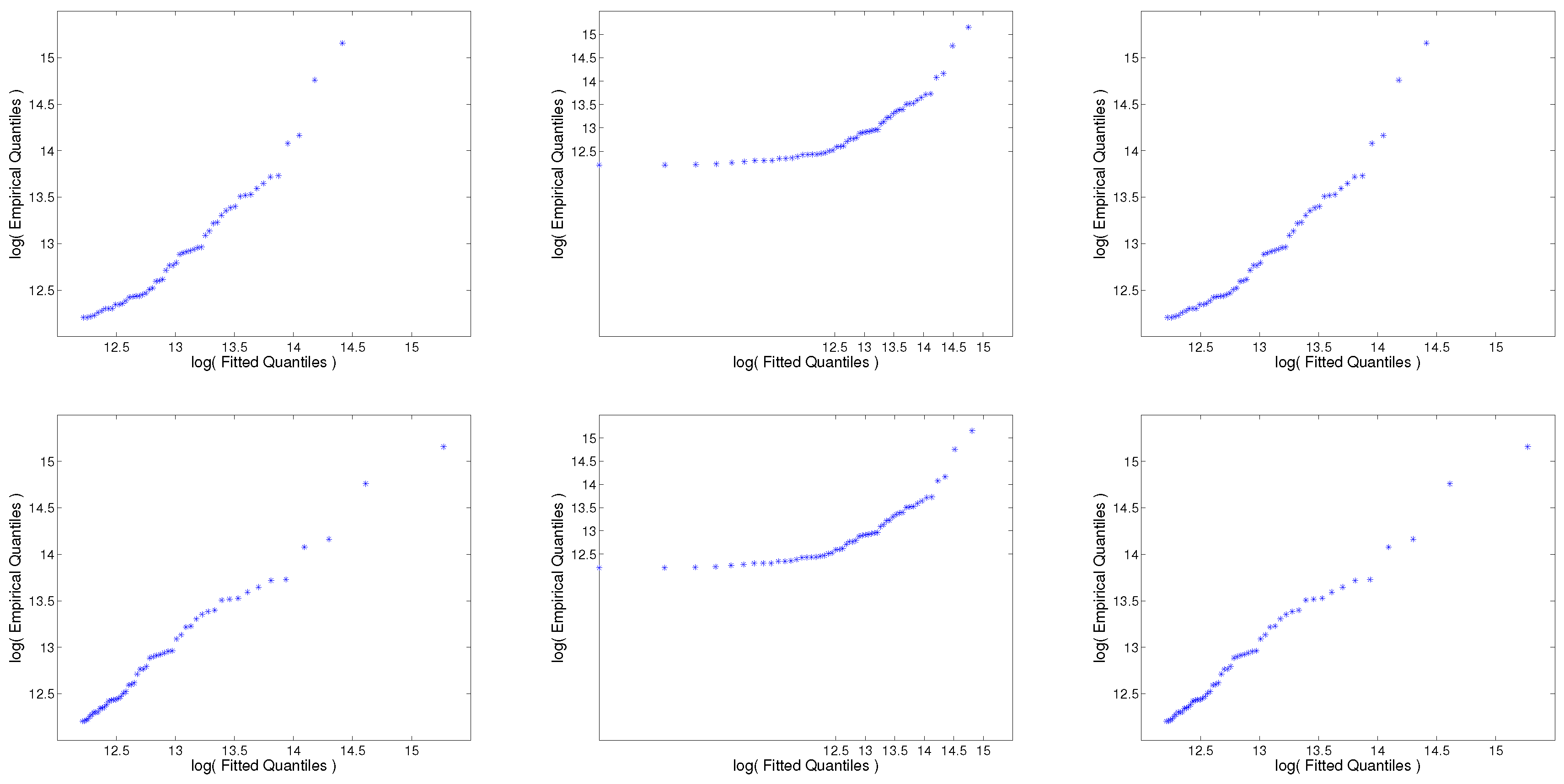
In Figure 2, we present plots of the fitted-versus-observed quantiles for the six models of Section 3.2. In order to avoid visual distortions due to large spacings between the most extreme observations, both axes in all the plots are measured on a logarithmic scale. That is, the points plotted in those graphs are the following pairs:

$$\left(log\left({\widehat{G}}^{-1}\left(u_i\right)\right),log\left(X_{\left(i\right)}\right)\right),i=1,\dots ,54,$$

where ${\widehat{G}}^{-1}$ is the estimated parametric qf, $X_{\left(1\right)}\le \cdots \le X_{\left(54\right)}$ denote the ordered losses, and $u_i=(i-0.5)/54$ is the quantile level. For the truncated approach, ${\widehat{G}}^{-1}\left(u_i\right)={\widehat{F}}^{-1}\left(u_i+\widehat{F}(195,000)(1-u_i)\right)$; for the naive approach, ${\widehat{G}}^{-1}\left(u_i\right)={\widehat{F}}^{-1}\left(u_i\right)$; for the shifted approach, ${\widehat{G}}^{-1}\left(u_i\right)={\widehat{F}}^{-1}\left(u_i\right)+195,000$. Additionally, the corresponding cdf and qf functions were evaluated using the MLE values from Table 4.

We can see from Figure 2 that Lomax models show a better overall fit than exponential models, and especially in the extreme right tail. That is, most of the points in those plots do not deviate from the ${45}^{\circ }$ line. The naive approach seems off, but the truncated and shifted approaches do a reasonably good job for both distributions, with Lomax models exhibiting slightly better fits.

The KS and AD goodness-of-fit statistics measure, respectively, the maximum absolute distance and the cumulative weighted quadratic distance (with more weight on the tails) between the empirical cdf ${\widehat{F}}_n\left(x\right)=n^{-1}{\sum }_{i=1}^n\mathbf{1}\{X_i\le x\}$ and the parametrically estimated cdf $\widehat{G}\left(x\right)$. Their respective computational formulas are given by

$${\mathrm{K}\mathrm{S}}_n=\underset{1\le i\le n}{max}\left\{|\widehat{G}\left(X_{\left(i\right)}\right)-\frac{i-1}{n}|,|\widehat{G}\left(X_{\left(i\right)}\right)-\frac{i}{n}|\right\}$$

and

$${\mathrm{A}\mathrm{D}}_n=-n+n\sum _{i=1}^n{\left(i/n\right)}^{2}log\left(\frac{\widehat{G}\left(X_{(i+1)}\right)}{\widehat{G}\left(X_{\left(i\right)}\right)}\right)-n\sum _{i=0}^{n-1}{\left(1-i/n\right)}^{2}log\left(\frac{1-\widehat{G}\left(X_{(i+1)}\right)}{1-\widehat{G}\left(X_{\left(i\right)}\right)}\right),$$

where $195,000=X_{\left(0\right)}\le X_{\left(1\right)}\le \cdots \le X_{\left(n\right)}\le X_{(n+1)}=\infty$ denote the ordered claim severities. Additionally, $\widehat{G}\left(X_{\left(i\right)}\right)={\widehat{F}}_{*}\left(X_{\left(i\right)}\right)$ for the truncated approach, $\widehat{G}\left(X_{\left(i\right)}\right)=\widehat{F}\left(X_{\left(i\right)}\right)$ for the naive approach, and $\widehat{G}\left(X_{\left(i\right)}\right)=\widehat{F}(X_{\left(i\right)}-195,000)$ for the shifted approach. Note that $n=54$ and the corresponding cdf’s were evaluated using the MLE values from Table 4. The p-values of the KS and AD tests were computed using parametric bootstrap with 10,000 simulation runs. For a brief description of the parametric bootstrap procedure, see, for example, Klugman, Panjer, and Willmot (2012, sct. 20.4.5).

As the results of

Table 5. Values of KS and AD statistics (with p-values in parentheses) for the fitted models, using truncated, naive, and shifted approaches.

Model	Kolmogorov–Smirnov			Anderson–Darling
	Truncated	Naive	Shifted	Truncated	Naive	Shifted
Exponential	$0.186$ (0.004)	$0.307$ (0.000)	$0.186$ (0.004)	$3.398$ (0.000)	$4.509$ (0.000)	$3.398$ (0.000)
Lomax	$0.072$ (0.632)	$0.316$ (0.000)	$0.072$ (0.631)	$0.272$ (0.671)	$4.696$ (0.000)	$0.272$ (0.678)

suggest, both naive models are strongly rejected by the KS and AD tests, which is consistent with the conclusions based on QQ-plots. The truncated and shifted exponential models are also rejected, which strengthens our “weak” decisions based on QQ-plots. Unfortunately, for this data set, neither KS nor the AD test can help us with differentiating between the truncated and shifted Lomax models, as both of them fit the data very well.

3.4. VaR Estimates

Having fitted and validated the models, we now compute several point and interval estimates of $\mathrm{VaR}\left(\beta \right)$ for all six models. The purpose of calculating $\mathrm{VaR}\left(\beta \right)$ estimates for all—“good” and “bad”—models is to see the impact that model fit (which is driven by the initial assumptions) has on the capital estimates. The results are summarized in

Table 6. Value-at-risk ($\mathrm{VaR}\left)\right(\beta )$ estimates (with 95% confidence intervals in parentheses), measured in millions and based on the fitted models, using truncated, naive, and shifted approaches.

Model	$\mathit{\beta }$	Truncated	Naive	Shifted
Exponential	0.95	1.052 (0.771; 1.332)	1.636 (1.199; 2.072)	1.247 (0.966; 1.527)
	0.995	1.860 (1.364; 2.356)	2.893 (2.121; 3.665)	2.055 (1.559; 2.551)
	0.999	2.425 (1.778; 3.071)	3.772 (2.766; 4.778)	2.620 (1.973; 3.266)
Lomax	0.95	0.576 (0.071; 1.160)	1.670 (1.134; 2.206)	1.514 (0.978; 2.755)
	0.995	2.281 (0.413; 4.758)	3.114 (2.257; 5.023)	5.417 (2.213; 20.604)
	0.999	5.504 (1.100; 13.627)	4.214 (3.019; 8.586)	12.797 (3.649; 89.992)

Empirical estimates of $\mathrm{VaR}\left(\beta \right)$: 1.416 (for $\beta =0.95$) and 3.822 (for $\beta =0.995$ and $0.999$).

, where empirical estimates of $\mathrm{VaR}\left(\beta \right)$ are also reported for completeness. The confidence intervals for the exponential models are derived using Theorem A3 and based on the variance estimates from Table 4. For the Lomax models, the confidence intervals are obtained using parametric bootstrap with 10,000 simulation runs.

We see from the table that the $\mathrm{VaR}\left(\beta \right)$ estimates based on the naive approach significantly differ from the rest. The difference between truncated and shifted estimates at the exponential model is $t=195,000$. For the Lomax model, these two approaches—which exhibited nearly perfect fits to data—produce substantially different estimates, especially at the very extreme tail. Finally, in view of such large differences between parametric estimates (which resulted from models with excellent fits), the empirical estimates do not seem completely off.

3.5. Model Predictions

As the final test of our models, we check their out-of-sample predictive power.

Table 7. Unobserved costs of legal events (below $195,000).

142,774.19	146,875.00	151,000.00	160,000.00	176,000.00	182,435.12	191,070.31
143,000.00	150,411.29	153,592.54	165,000.00	176,000.00	185,000.00	192,806.74
145,500.50	150,930.39	157,083.00	165,000.00	180,000.00	186,330.00	193,500.00

Source: Cruz (2002, p. 57).

provides the “unobserved” legal losses, which will be used to verify how accurate our model-based predictions are. To start with, we note that the empirical and shifted models are not able to produce meaningful predictions because they assume that such data were impossible to occur (i.e., $\widehat{F}(195,000)=0$ for these two approaches). So, we now work only with the truncated and naive models.

Firstly, we report the estimated probabilities of losses below the data collection threshold, $\widehat{F}(195,000)$. For the exponential models, it is 0.300 (naive) and 0.426 (truncated). For the Lomax models, it is 0.310 (naive) and 0.794 (truncated). Secondly, using these probabilities we can estimate the total, observed, and unobserved number of losses. For the exponential models, $\widehat{N}=77.2\approx 77$ (naive) and $\widehat{N}=94.1\approx 94$ (truncated). For the Lomax models, $\widehat{N}=78.3\approx 78$ (naive) and $\widehat{N}=262.1\approx 262$ (truncated). Note how different from the rest the estimate of the truncated Lomax model is. (Recall that this model exhibited the best statistical fit for the observed data).

For predictions that are verifiable, in

Table 8. Model-based predictions (with 95% confidence intervals in parentheses) of several statistics for the unobserved losses between $150,000 and $175,000.

Model	Truncated			Naive
	Number of Losses	Average Loss	Total Loss	Number of Losses	Average Loss	Total Loss
Exponential	4.2	162,352	685,108	2.6	162,405	426,197
	(3.0; 5.5)	(162,312; 162,391)	(452,840; 917,376)	(1.9; 3.4)	(162,379; 162,430)	(141,592; 710,802)
Lomax	9.9	162,017	1,609,649	2.7	162,397	441,155
	(3.3; 16.5)	(161,647; 162,388)	(543,017; 2,676,281)	(1.8; 3.7)	(162,343; 162,451)	(288,324; 593,985)

we report model-based estimates of the number of losses, the average loss, and the total loss in the interval [150,000;175,000]. We also provide the corresponding 95% confidence intervals for the predictions. The intervals were constructed by using the variance and covariance estimates of Table 4 in conjunction with Theorem A3. Notice that by using the data points from Table 7 it is straightforward to verify that the actual number of losses is eight, the average loss is 156,627, and the total loss is 1,253,017. We see from Table 8 that, with the exception of the average loss measure, there are large disparities in predictions between different approaches. This mostly has to do with the quality of model fit for the given data set, which is good for the truncated Lomax model but bad for the other models and/or approaches. As a consequence, 95% confidence intervals based on the truncated Lomax model cover the actual values of two important measures—number of losses (eight) and total loss (1,253,017)—but those based on the truncated exponential model do not. Moreover, both naive models fit the data poorly and produce point and interval predictions that are even further from their respective targets than those of the truncated exponential model. In addition, if one chose to ignore the model validation step and proceeded directly to predictions based on the naive models, they would be (falsely) reassured by the consistency of such predictions (number of losses: 2.6 and 2.7; total loss: 426,197 and 441,155).

4. Concluding Remarks

In this paper, we have studied the problem of model uncertainty in operational risk modeling, which arises due to different (seemingly plausible) model assumptions. We have focused on the statistical aspects of the problem by utilizing asymptotic theorems of mathematical statistics, Monte Carlo simulations, and real-data examples. Similar to other authors who have studied some aspects of this topic before, we conclude that:

• The naive and empirical approaches are inappropriate for determining VaR estimates.
• The shifted approach—although fundamentally flawed (simply because it assumes that operational losses below the data collection threshold are impossible)—has the flexibility to adapt to data well and successfully pass standard model validation tests.
• The truncated approach is theoretically sound when appropriate fits data well, and (in our examples) produces lower VaR-based capital estimates than those of the shifted approach.

The research presented in this paper invites follow-up studies in several directions. For example, as the first and most obvious direction, one may choose to explore these issues for other—perhaps more popular in practice—distributions such as lognormal or loggamma. If the chosen model lends itself to analytic investigations, then our Example 1 (in Section 2.3) is a blueprint for analysis. Otherwise, one may follow our Example 2 for a simulations-based approach. Second, VaR can be replaced by a different risk measure. For instance, the Expected Shortfall (also known as Tail-VaR or Conditional Tail Expectation) has some theoretical advantages over VaR (e.g., it is a coherent risk measure), and is a recommended measure in the Swiss Solvency Test. Third, due to the theoretical soundness of the truncated approach, one may try to develop model-selection strategies for truncated (but not necessarily nested) models. However, this line of work may be quite challenging due to the “flatness” of the truncated likelihoods—a phenomenon frequently encountered in practice (see Cope 2011). The fourth venue of research that may also help with the latter problem is robust model fitting. There are several excellent contributions to this topic in the operational risk literature (e.g., Chau 2013; Horbenko et al. 2011; Opdyke and Cavallo 2012), but more work can be done.

References

- AMA Group. 2013. AMA Quantification Challenges: AMAG Range of Practice and Observations on “The Thorny LDA Topics”. Munich: Risk Management Association. [Google Scholar]
- Arnold, Barry C. 2015. Pareto Distributions, 2nd ed. London: Chapman & Hall. [Google Scholar]
- Basel Coordination Committee. 2014. Supervisory guidance for data, modeling, and model risk management under the operational risk advanced measurement approaches. Basel Coordination Committee Bulletin 14: 1–17. [Google Scholar]
- Baud, Nicolas, Antoine Frachot, and Thierry Roncalli. 2002. Internal Data, External Data and Consortium Data for Operational Risk Measurement: How to Pool Data Properly? Working Paper, Groupe de Recherche Opérationnelle, Crédit Lyonnais, France. [Google Scholar]
- Brazauskas, Vytaras, Bruce L. Jones, and Ričardas Zitikis. 2015. Trends in disguise. Annals of Actuarial Science 9: 58–71. [Google Scholar] [CrossRef]
- Cavallo, Alexander, Benjamin Rosenthal, Xiao Wang, and Jun Yan. 2012. Treatment of the data collection threshold in operational risk: A case study with the lognormal distribution. Journal of Operational Risk 7: 3–38. [Google Scholar] [CrossRef]
- Chau, Joris. 2013. Robust Estimation in Operational Risk Modeling. Master’s thesis, Department of Mathematics, Utrecht University, Utrecht, The Netherland. [Google Scholar]
- Chernobai, Anna S., Svetlozar T. Račev, and Frank J. Fabozzi. 2007. Operational Risk: A Guide to Basel II Capital Requirements, Models, and Analysis. Hoboken: Wiley. [Google Scholar]
- Cope, Eric. 2011. Penalized likelihood estimators for truncated data. Journal of Statistical Planning and Inference 141: 345–58. [Google Scholar] [CrossRef]
- Cruz, Marcelo G. 2002. Modeling, Measuring and Hedging Operational Risk. Hoboken: Wiley. [Google Scholar]
- Cruz, Marcelo G., Gareth W. Peters, and Pavel V. Shevchenko. 2015. Fundamental Aspects of Operational Risk and Insurance Analytics: A Handbook of Operational Risk. Hoboken: Wiley. [Google Scholar]
- De Fontnouvelle, Patrick, Virginia Dejesus-Rueff, John S. Jordan, and Eric S. Rosengren. 2006. Capital and risk: New evidence on implications of large operational losses. Journal of Money, Credit, and Banking 38: 1819–46. [Google Scholar] [CrossRef]
- Ergashev, Bakhodir, Konstantin Pavlikov, Stan Uryasev, and Evangelos Sekeris. 2016. Estimation of truncated data samples in operational risk modeling. Journal of Risk and Insurance 83: 613–40. [Google Scholar] [CrossRef]
- Horbenko, Nataliya, Peter Ruckdeschel, and Taehan Bae. 2011. Robust estimation of operational risk. Journal of Operational Risk 6: 3–30. [Google Scholar] [CrossRef]
- Klugman, Stuart A., Harry Panjer, and Gordon E. Willmot. 2012. Loss Models: From Data to Decisions, 4th ed. Hoboken: Wiley. [Google Scholar]
- Luo, Xiaolin, Pavel V. Shevchenko, and John B. Donnelly. 2007. Addressing the impact of data truncation and parameter uncertainty on operational risk estimates. Journal of Operational Risk 2: 3–26. [Google Scholar] [CrossRef]
- Moscadelli, Marco, Anna Chernobai, and Svetlozar T. Rachev. 2005. Treatment of missing data in the field of operational risk: The impacts on parameter estimates, EL and UL figures. Operational Risk 6: 28–34. [Google Scholar]
- Office of the Comptroller of the Currency. 2011. Supervisory guidance on model risk management. SR Letter 11: 1–21. [Google Scholar]
- Opdyke, John Douglas. 2014. Estimating operational risk capital with greater accuracy, precision, and robustness. Journal of Operational Risk 9: 3–79. [Google Scholar] [CrossRef]
- Opdyke, John Douglas, and Alexander Cavallo. 2012. Estimating operational risk capital: The challenges of truncation, the hazards of maximum likelihood estimation, and the promise of robust statistics. Journal of Operational Risk 7: 3–90. [Google Scholar] [CrossRef]
- Serfling, Robert J. 1980. Approximation Theorems of Mathematical Statistics. Hoboken: Wiley. [Google Scholar]
- Shevchenko, Pavel V., and Grigory Temnov. 2009. Modeling operational risk data reported above a time-varying threshold. Journal of Operational Risk 4: 19–42. [Google Scholar] [CrossRef]
Figure 1.
Truncated, naive, and shifted and probability density functions. Data collection threshold , with 50% of data unobserved. Parameters and are chosen to match those in Tables 2 and 3 (see Section 2.3).
Figure 2.
Fitted-versus-observed log-losses for exponential (top row) and Lomax (bottom row) distributions, using truncated (left), naive (middle), and shifted (right) approaches.