Appendix A. Autoregressive Integrated Moving Average
The autoregressive integrated moving average (ARIMA) model (
Box et al. 1994) is commonly used to forecast nonstationary time series. The assumption to apply an ARIMA
model is that after differencing
d times the input time series, the obtained values
are a stationary time series with zero mean. It is also assumed that future values of this time series are a linear function of
p past observations
and
q past errors
.
The ARIMA
model is thus expressed as follows:
where
,...,
are the parameters of the autoregressive part of the model,
,...,
are the parameters of the moving average part and the error is defined by
. The order of the model is defined by the values of
p and
q, which are identified from the autocorrelation function and the partial autocorrelation function (
Brockwell and Davis 2002). The model parameters,
and
, are estimated using the maximum likelihood method.
Appendix B. Results for m = 1 and m = 5
For comparison, we report the results for input vectors of lengths
and
.
Table A1 and
Table A2 correspond to
and
, respectively, and they must be compared with the results reported for
in
Table 2.
Figure A1 and
Figure A2 correspond to
and
, respectively, and they must be compared with the results reported for
in
Figure 5.
Table A3 and
Table A4 correspond to
and
, respectively, and they must be compared with the results reported for
in
Table 3.
Table A1.
Mean absolute error (MAE): mean and standard deviation (std) for the considered forecasting models with input vector lagged values. The smallest MAE of each forecast horizon is set in boldface.
Table A1.
Mean absolute error (MAE): mean and standard deviation (std) for the considered forecasting models with input vector lagged values. The smallest MAE of each forecast horizon is set in boldface.
| Steps Ahead h | 1 | 2 | 3 | 5 | 10 | 20 | 30 | 50 |
|---|
| Model | Mean | Std | Mean | Std | Mean | Std | Mean | Std | Mean | Std | Mean | Std | Mean | Std | Mean | Std |
|---|
| Benchmarks | Naive | 0.147 | (0.186) | 0.256 | (0.322) | 0.328 | (0.418) | 0.423 | (0.514) | 0.651 | (0.801) | 0.991 | (1.053) | 1.143 | (1.294) | 1.559 | (1.803) |
| ARIMA | 0.145 | (0.185) | 0.247 | (0.303) | 0.313 | (0.374) | 0.421 | (0.477) | 0.663 | (0.783) | 1.021 | (1.035) | 1.154 | (1.304) | 1.644 | (1.789) |
| Direct SVR | 0.204 | (0.200) | 0.313 | (0.395) | 0.378 | (0.473) | 0.529 | (0.610) | 0.832 | (1.040) | 1.270 | (1.380) | 1.540 | (1.587) | 2.185 | (2.336) |
| Recursive SVR | 0.204 | (0.200) | 0.283 | (0.365) | 0.324 | (0.412) | 0.439 | (0.556) | 0.628 | (0.831) | 0.986 | (1.140) | 1.077 | (1.221) | 1.599 | (1.868) |
| Direct EMD–SVR | Multivariate | 0.162 | (0.180) | 0.264 | (0.317) | 0.330 | (0.374) | 0.417 | (0.484) | 0.650 | (0.718) | 0.921 | (1.010) | 1.229 | (1.292) | 1.642 | (1.947) |
| 0.196 | (0.205) | 0.308 | (0.356) | 0.378 | (0.425) | 0.491 | (0.504) | 0.748 | (0.805) | 1.180 | (1.259) | 1.498 | (1.361) | 1.903 | (2.103) |
| 0.196 | (0.198) | 0.304 | (0.354) | 0.376 | (0.432) | 0.489 | (0.502) | 0.747 | (0.803) | 1.181 | (1.258) | 1.498 | (1.362) | 1.903 | (2.102) |
| 0.243 | (0.244) | 0.310 | (0.345) | 0.384 | (0.433) | 0.490 | (0.514) | 0.749 | (0.806) | 1.180 | (1.259) | 1.505 | (1.362) | 1.904 | (2.098) |
| 0.380 | (0.430) | 0.436 | (0.452) | 0.478 | (0.483) | 0.543 | (0.532) | 0.799 | (0.867) | 1.198 | (1.265) | 1.488 | (1.349) | 1.919 | (2.093) |
| 0.616 | (0.677) | 0.657 | (0.712) | 0.691 | (0.709) | 0.730 | (0.764) | 0.869 | (1.021) | 1.218 | (1.317) | 1.506 | (1.382) | 1.915 | (2.085) |
| R | 0.890 | (0.971) | 0.924 | (0.989) | 0.934 | (0.946) | 0.964 | (0.966) | 1.033 | (1.076) | 1.297 | (1.358) | 1.546 | (1.505) | 1.924 | (2.036) |
| Recursive EMD–SVR | Multivariate | — | — | — | — | — | — | — | — | — | — | — | — | — | — | — | — |
| 0.196 | (0.205) | 0.278 | (0.331) | 0.333 | (0.432) | 0.416 | (0.474) | 0.633 | (0.774) | 0.939 | (1.036) | 1.143 | (1.307) | 1.545 | (1.775) |
| 0.196 | (0.198) | 0.279 | (0.331) | 0.333 | (0.432) | 0.415 | (0.474) | 0.631 | (0.774) | 0.940 | (1.036) | 1.143 | (1.307) | 1.545 | (1.775) |
| 0.243 | (0.244) | 0.301 | (0.332) | 0.354 | (0.402) | 0.437 | (0.469) | 0.653 | (0.770) | 0.950 | (1.035) | 1.158 | (1.312) | 1.557 | (1.789) |
| 0.380 | (0.430) | 0.431 | (0.444) | 0.458 | (0.471) | 0.514 | (0.508) | 0.710 | (0.775) | 1.010 | (1.074) | 1.209 | (1.309) | 1.621 | (1.800) |
| 0.616 | (0.677) | 0.647 | (0.708) | 0.675 | (0.695) | 0.685 | (0.741) | 0.816 | (0.982) | 1.076 | (1.237) | 1.295 | (1.282) | 1.644 | (1.851) |
| R | 0.890 | (0.971) | 0.920 | (0.987) | 0.923 | (0.940) | 0.937 | (0.951) | 0.989 | (1.049) | 1.209 | (1.237) | 1.414 | (1.389) | 1.721 | (1.848) |
Table A2.
Mean absolute error (MAE) and standard deviation (std) for the considered forecasting models: naive, autoregressive integrated moving average (ARIMA), univariate and multivariate empirical mode decomposition–support vector regression (EMD–SVR) with input vector lagged values. The smallest MAE of each forecast horizon is set in boldface.
| Steps Ahead h | 1 | 2 | 3 | 5 | 10 | 20 | 30 | 50 |
|---|
| Model | Mean | Std | Mean | Std | Mean | Std | Mean | Std | Mean | Std | Mean | Std | Mean | Std | Mean | Std |
|---|
| Benchmarks | Naive | 0.147 | (0.186) | 0.256 | (0.322) | 0.328 | (0.418) | 0.423 | (0.514) | 0.651 | (0.801) | 0.991 | (1.053) | 1.143 | (1.294) | 1.559 | (1.803) |
| ARIMA | 0.145 | (0.185) | 0.247 | (0.303) | 0.313 | (0.374) | 0.421 | (0.477) | 0.663 | (0.783) | 1.021 | (1.035) | 1.154 | (1.304) | 1.644 | (1.789) |
| Direct SVR | 0.145 | (0.146) | 0.242 | (0.289) | 0.294 | (0.362) | 0.408 | (0.450) | 0.615 | (0.723) | 0.943 | (0.981) | 1.101 | (1.201) | 1.641 | (1.733) |
| Recursive SVR | 0.145 | (0.146) | 0.257 | (0.357) | 0.393 | (0.566) | 0.577 | (0.841) | 1.080 | (1.922) | 1.228 | (1.939) | 1.338 | (2.054) | 1.627 | (2.366) |
| Direct EMD–SVR | Multivariate | 0.144 | (0.180) | 0.222 | (0.289) | 0.284 | (0.353) | 0.379 | (0.448) | 0.585 | (0.711) | 0.866 | (0.928) | 1.017 | (1.153) | 1.379 | (1.585) |
| 0.120 | (0.146) | 0.181 | (0.226) | 0.234 | (0.278) | 0.371 | (0.426) | 0.557 | (0.667) | 0.874 | (0.896) | 1.024 | (1.046) | 1.430 | (1.601) |
| 0.124 | (0.138) | 0.182 | (0.228) | 0.234 | (0.286) | 0.371 | (0.421) | 0.557 | (0.658) | 0.879 | (0.898) | 1.023 | (1.049) | 1.433 | (1.602) |
| 0.173 | (0.184) | 0.217 | (0.240) | 0.247 | (0.283) | 0.373 | (0.387) | 0.556 | (0.637) | 0.886 | (0.910) | 1.029 | (1.053) | 1.441 | (1.611) |
| 0.277 | (0.324) | 0.316 | (0.331) | 0.334 | (0.349) | 0.389 | (0.390) | 0.544 | (0.604) | 0.795 | (0.848) | 0.916 | (0.930) | 1.298 | (1.425) |
| 0.449 | (0.495) | 0.471 | (0.519) | 0.491 | (0.511) | 0.503 | (0.536) | 0.594 | (0.714) | 0.788 | (0.903) | 0.927 | (0.916) | 1.258 | (1.393) |
| R | 0.655 | (0.709) | 0.675 | (0.725) | 0.679 | (0.694) | 0.688 | (0.707) | 0.729 | (0.782) | 0.788 | (0.811) | 0.908 | (0.876) | 1.167 | (1.234) |
| Recursive EMD–SVR | Multivariate | — | — | — | — | — | — | — | — | — | — | — | — | — | — | — | — |
| 0.120 | (0.1460) | 0.241 | (0.321) | 0.383 | (0.463) | 0.634 | (0.813) | 0.829 | (0.915) | 1.077 | (1.138) | 1.298 | (1.391) | 1.807 | (1.949) |
| 0.124 | (0.138) | 0.239 | (0.302) | 0.381 | (0.460) | 0.612 | (0.820) | 0.826 | (0.921) | 1.085 | (1.153) | 1.299 | (1.389) | 1.806 | (1.950) |
| 0.173 | (0.184) | 0.245 | (0.299) | 0.370 | (0.442) | 0.535 | (0.703) | 0.823 | (0.909) | 1.082 | (1.143) | 1.341 | (1.410) | 1.807 | (1.939) |
| 0.277 | (0.324) | 0.315 | (0.312) | 0.383 | (0.380) | 0.544 | (0.560) | 0.724 | (0.791) | 1.076 | (1.123) | 1.327 | (1.390) | 1.777 | (1.906) |
| 0.449 | (0.495) | 0.464 | (0.501) | 0.482 | (0.497) | 0.522 | (0.552) | 0.673 | (0.773) | 0.929 | (1.070) | 1.211 | (1.329) | 1.736 | (1.896) |
| R | 0.655 | (0.709) | 0.666 | (0.709) | 0.657 | (0.669) | 0.651 | (0.674) | 0.736 | (0.756) | 0.962 | (1.019) | 1.134 | (1.240) | 1.523 | (1.887) |
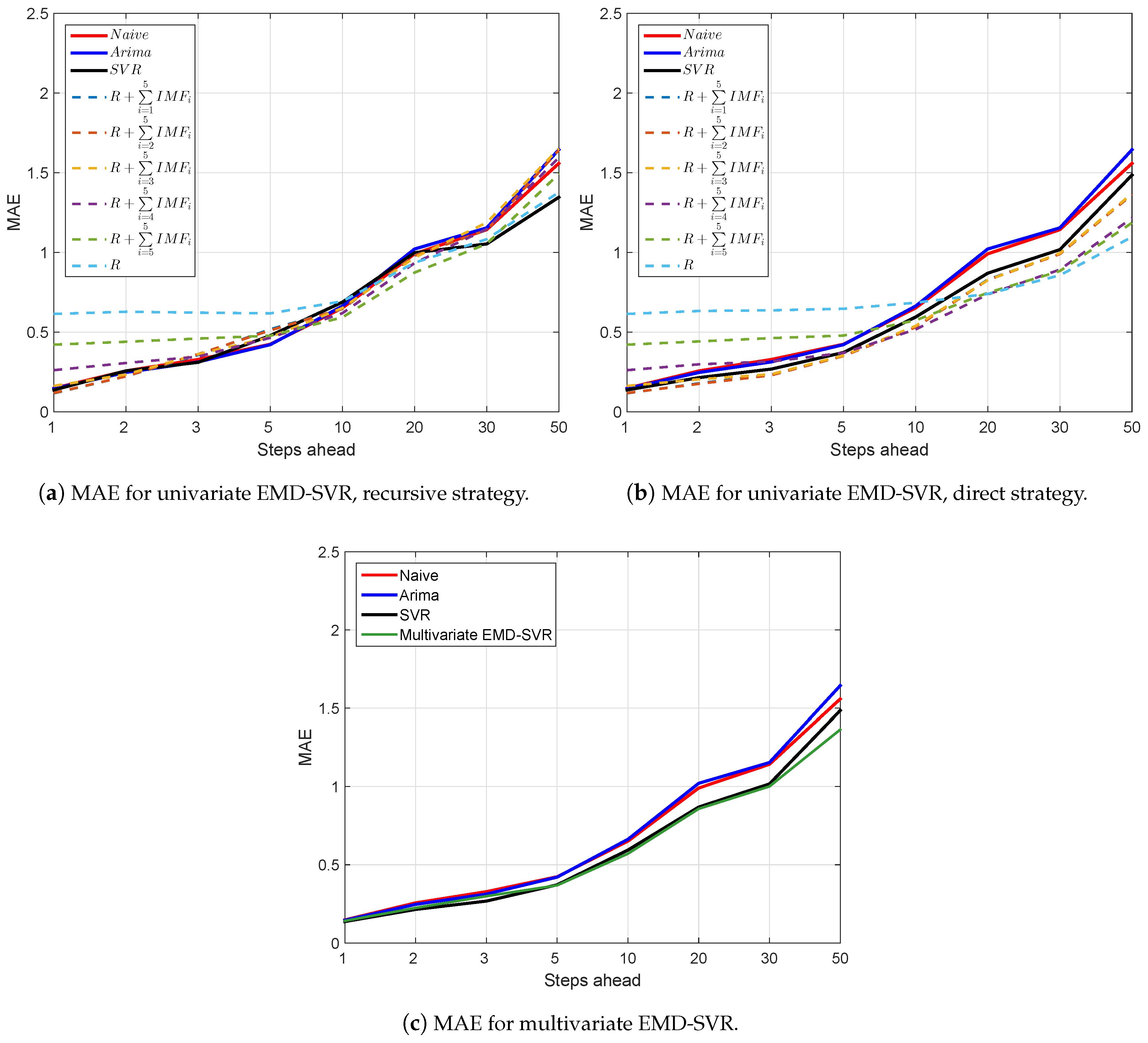
Figure A1.
Mean absolute error (MAE) as a function of the forecast horizon for the considered forecasting models: naive, autoregressive integrated moving average (ARIMA), and univariate and multivariate empirical mode decomposition–support vector regression (EMD–SVR) with input vector lagged values.
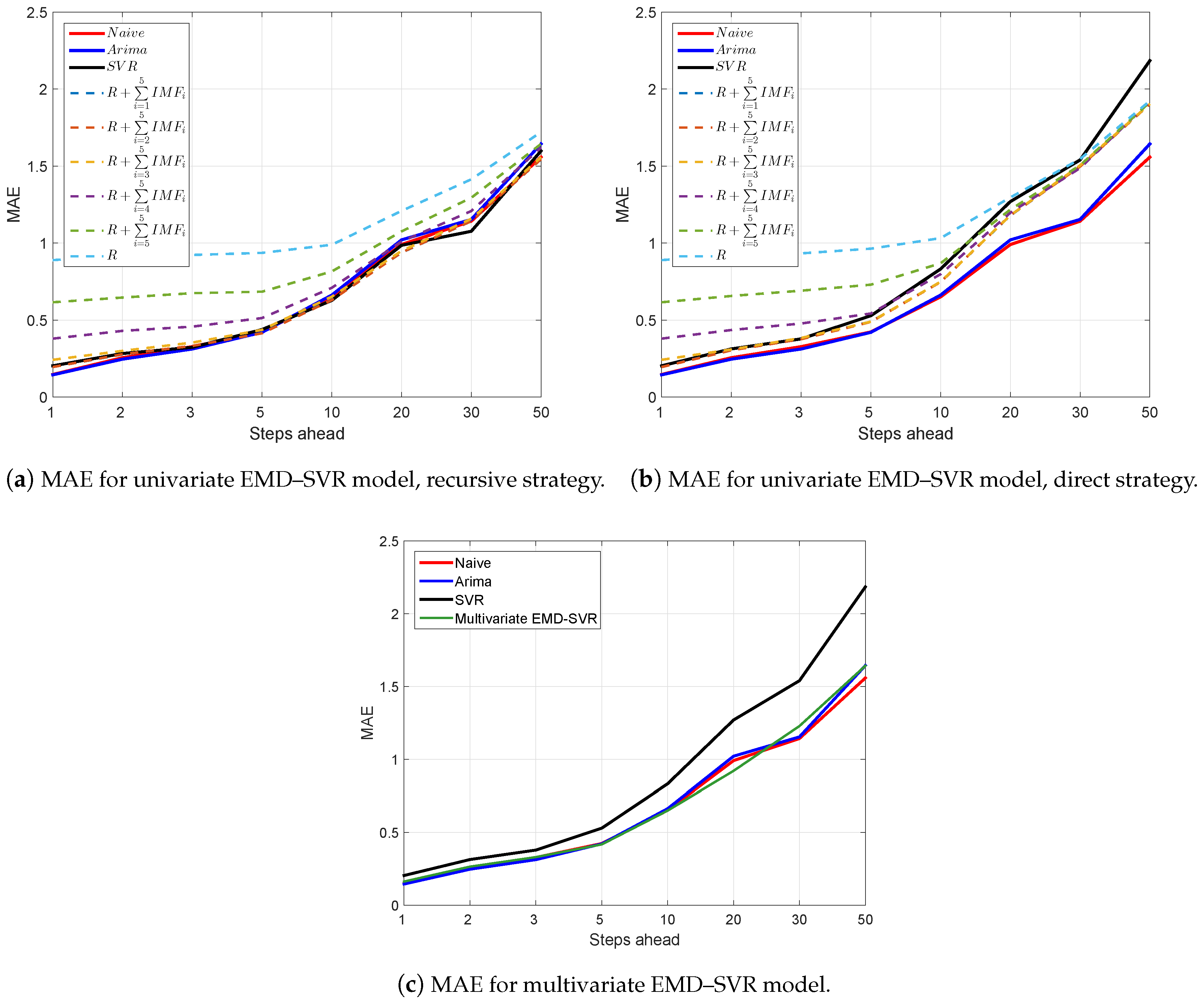
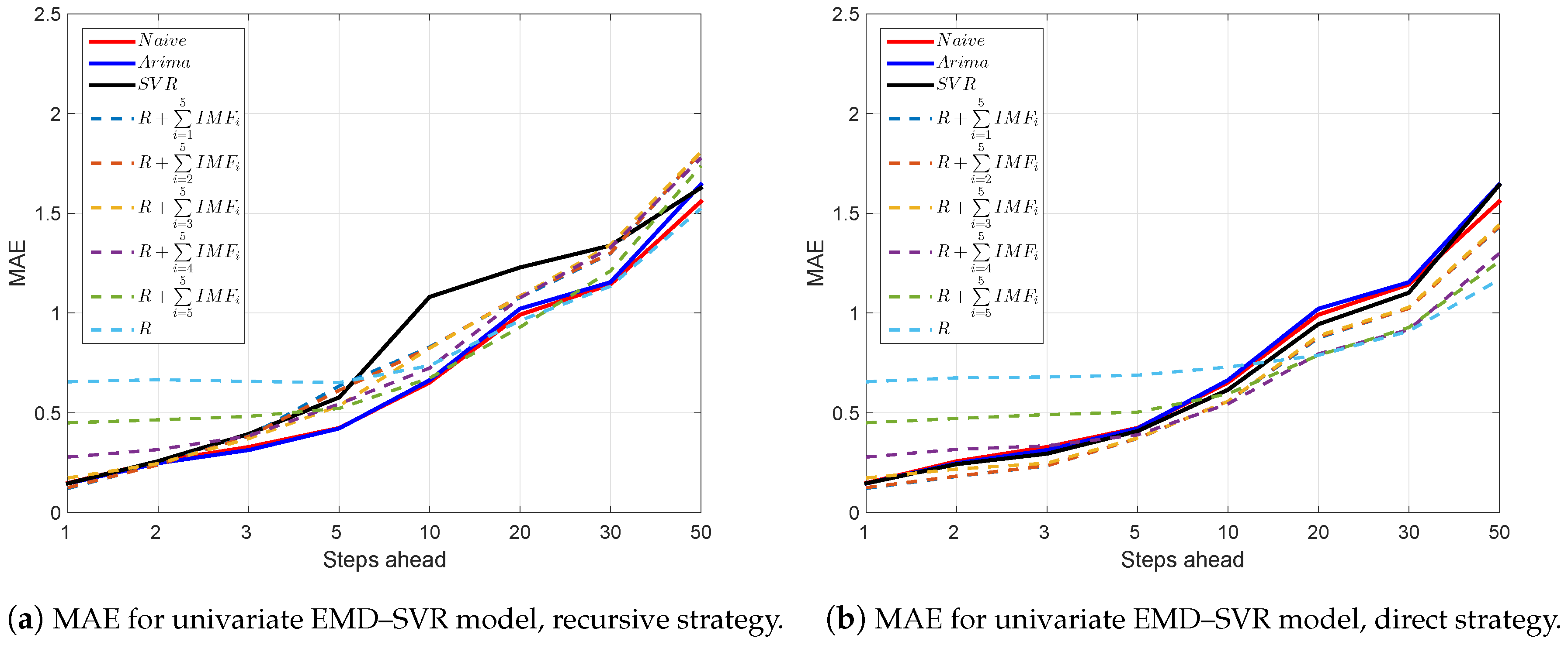
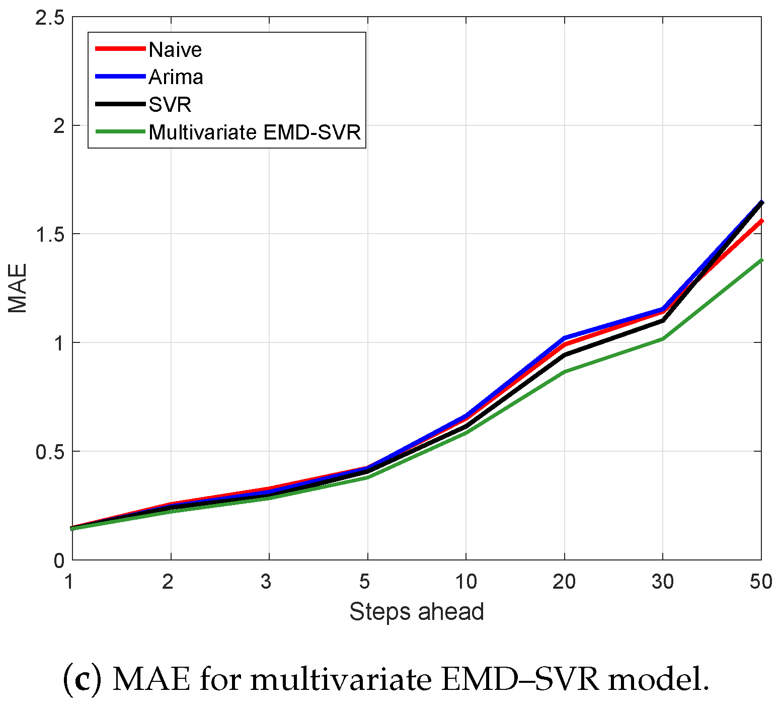
Figure A2.
Mean absolute error (MAE) as a function of the forecast horizon for the considered forecasting models: naive, autoregressive integrated moving average (ARIMA), univariate and multivariate empirical mode decomposition–support vector regression (EMD–SVR) with input vector lagged values.
Figure A2.
Mean absolute error (MAE) as a function of the forecast horizon for the considered forecasting models: naive, autoregressive integrated moving average (ARIMA), univariate and multivariate empirical mode decomposition–support vector regression (EMD–SVR) with input vector lagged values.
Table A3.
Z-statistic for the Wilcoxon signed-rank test for the null hypothesis that the naive model is as accurate as the studied models: autoregressive integrated moving average (ARIMA), and univariate and multivariate empirical mode decomposition–support vector regression (EMD–SVR) with input vector . Top: direct strategy; bottom: recursive strategy. * Statistically significant at the 5% confidence level. ** Statistically significant at the 1% confidence level.
| Model\Steps Ahead h | 1 | 2 | 3 | 5 | 10 | 20 | 30 | 50 |
|---|
| Benchmarks | ARIMA | −0.22 | 0.16 | 0.89 | 0.30 | −1.45 | −1.59 | −0.49 | −1.47 |
| Direct SVR | −4.72 ** | −3.05 ** | −2.54 * | −3.24 ** | −3.47 ** | −2.75 ** | −3.35 ** | −3.39 ** |
| Recursive SVR | −4.72 ** | −1.83 | −0.44 | −0.58 | 0.03 | 1.01 | 1.37 | 0.27 |
| Direct EMD–SVR | Multivariate | −1.83 | −0.80 | −0.39 | 0.94 | 0.22 | 1.37 | −0.18 | 1.41 |
| −4.07 ** | −3.07 ** | −3.11 * | −2.96 ** | −2.72 ** | −2.11 * | −3.70 ** | −2.32 * |
| −4.21 ** | −3.12 ** | −2.84 ** | −2.88 ** | −2.73 ** | −2.12 * | −3.71 ** | −2.32 * |
| −5.62 ** | −3.18 ** | −2.99 ** | −2.60 ** | −2.69 ** | −2.12 * | −3.74 ** | −2.37 * |
| −7.25 ** | −5.73 ** | −4.65 ** | −3.48 ** | −3.37 ** | −2.33 * | −3.51 ** | −2.45 * |
| −8.35 ** | −7.51 ** | −6.36 ** | −4.99 ** | −3.84 ** | −2.46 * | −3.20 ** | −2.47 * |
| R | −9.06 ** | −8.14 ** | −7.84 ** | −7.00 ** | −5.51 ** | −3.10 ** | −3.66 ** | −2.66 ** |
| Recursive EMD–SVR | Multivariate | — | — | — | — | — | — | — | — |
| −4.07 ** | −1.96 | −0.41 | −0.21 | 0.63 | 1.95 | 0.90 | 1.55 |
| −4.21 ** | −2.08 * | −0.62 | −0.13 | 0.76 | 1.93 | 0.92 | 1.51 |
| −5.62 ** | −2.82 ** | −1.76 | −1.11 | −0.09 | 1.44 | 0.43 | 1.34 |
| −7.25 ** | −5.55 ** | −4.48 ** | −3.38 ** | −2.17 * | −1.09 | −1.05 | −0.10 |
| −8.35 ** | −7.33 ** | −6.28 ** | −4.46 ** | −2.95 ** | −1.18 | −1.90 | 0.11 |
| R | −9.06 ** | −8.13 ** | −7.77 ** | −6.78 ** | −5.25 ** | −2.26 * | −2.84 ** | −0.86 |
Table A4.
Z-statistic for the Wilcoxon signed-rank test for the null hypothesis that the naive model is as accurate as the studied models: autoregressive integrated moving average (ARIMA), univariate and multivariate empirical mode decomposition–support vector regression (EMD–SVR) with input vector . Top: direct strategy; bottom: recursive strategy. * Statistically significant at the 5% confidence level. ** Statistically significant at the 1% confidence level.
| Model\Steps Ahead h | 1 | 2 | 3 | 5 | 10 | 20 | 30 | 50 |
|---|
| Benchmarks | ARIMA | −0.22 | 0.16 | 0.89 | 0.30 | −1.45 | −1.59 | −0.49 | −1.47 |
| Direct SVR | −0.45 | 1.08 | 1.54 | 0.72 | 0.57 | 1.24 | 0.67 | 0.14 |
| Recursive SVR | −0.45 | 1.53 | 1.15 | 0.87 | 0.36 | 1.79 | 1.59 | 2.29 * |
| Direct EMD–SVR | Multivariate | 0.20 | 5.58 ** | 4.70 ** | 4.57 ** | 5.67 ** | 8.43 ** | 7.70 ** | 7.66 ** |
| 3.33 ** | 6.71 ** | 6.41 ** | 3.17 ** | 2.79 ** | 2.79 ** | 1.61 | 2.39 ** |
| 2.49 * | 5.94 ** | 6.24 ** | 3.21 ** | 2.64 ** | 2.72 ** | 1.70 | 2.37 * |
| −1.94 | 1.88 | 3.93 ** | 1.75 | 1.94 | 2.54 * | 1.66 | 2.31 * |
| −5.66 ** | −2.31 * | −0.47 | 0.59 | 2.57 * | 4.02 ** | 3.99 ** | 3.55 ** |
| −7.45 ** | −5.54 ** | −3.82 ** | −1.76 | 0.61 | 3.56 ** | 3.42 ** | 3.98 ** |
| R | −8.59 ** | −7.12 ** | −6.28 ** | −4.12 ** | −2.12 * | 3.37 ** | 3.19 ** | 4.10 ** |
| Recursive EMD–SVR | Multivariate | — | — | — | — | — | — | — | — |
| 3.33 ** | 1.43 | −0.51 | −2.26 * | −1.31 | −0.15 | −0.95 | −1.24> |
| 2.49 * | 1.45 | −0.49 | −1.98 * | −1.23 | −0.08 | −1.02 | −1.19 |
| −1.94 | 1.03 | 0.11 | −1.32 | −1.38 | −0.22 | −1.33 | −1.31 |
| −5.66 ** | −2.30 * | −1.72 | −2.38 * | −0.73 | 0.07 | −1.18 | −1.28 |
| −7.45 ** | −5.59 ** | −3.86 ** | −2.01 * | −0.03 | 2.14 * | 0.34 | −1.00 |
| R | −8.59 ** | −7.13 ** | −6.06 ** | −3.86 ** | −2.11 * | 1.55 | 1.04 | 1.22 |


