Analyzing the Risks Embedded in Option Prices with rndfittool

Abstract

This paper introduces a new computational tool for the analysis of the risks embedded in a set of prices of European-style options. The software enables the estimation of the risk-neutral density (RND) from the observed option prices by means of orthogonal polynomial expansions. Orthogonal polynomials offer a viable alternative to more standard techniques based on interpolation and estimation of the second-order derivatives of option prices. The app rndfittool is available on GitHub and its usage is illustrated with examples based on real data.

1. Introduction

In response to the financial instability witnessed in the most recent years, regulators now require that risks, associated with changing economic and political conditions, are properly covered (hedged) by the institutional investors and investment banks. These risks can be directly covered by means of derivatives, which are special insurance contracts and can be seen as bets on the future states of the world. In other words, their prices depend on the probability of a certain scenario becoming reality. The probability of each of these scenarios, compensated by the investors’ attitude to risk, determines the risk-neutral density (RND). The RND serves as a fundamental tool to ensure that no-arbitrage opportunities arise in the market. For example, financial analysts often rely on the RND to price contracts that are traded over-the-counter, for which it would be otherwise difficult to determine whether an agreed-upon price favors the buyer or the seller. Additionally, the RND can be employed as a hedging tool, as it fully characterizes how an option’s price will respond to changes in the price of the underlying asset, see Bates (2005) and Alexander and Nogueira (2007) among others. Finally, the RND can be adopted to derive risk measures accounting for the investors’ attitude to risk, see Aït-Sahalia and Lo (2000).

It is common practice to compute the RND by means of a pricing model with parameter values calibrated on historical market data. Unfortunately, relying on parametric pricing models to estimate the RND might present several drawbacks, such as long processing time and potential biases arising from model misspecification. On one hand, simple models can be calibrated faster, but they tend to be inconsistent with some of the empirical properties characterizing financial data, thus producing biased results. On the other hand, more sophisticated models may take a long time to calibrate since no closed-form solutions are typically available. As alternative to parametric pricing models, Breeden and Litzenberger (1978) point out that the RND associated with a fixed time horizon can be inferred from current rather than historical data. More specifically, the RND can be extrapolated from a -sufficiently dense- set of observed call and put prices, also known as “vanilla options”. Notably, this relation does not prescribe parametric forms of any kind nor it imposes specific assumptions on the dynamic evolution of the underlying process. A popular and robust approach to implement the results of Breeden and Litzenberger (1978) is to approximate the RND by a simple probability density function (kernel), which is then corrected by a linear combination of special functions, called orthogonal polynomials. Under mild assumptions on the tail behavior of the RND it can be shown that the correction delivered by orthogonal polynomials is sufficient to recover the RND, irrespective of its closeness to the kernel. Therefore, this approach is very flexible and can be intended as (semi) non-parametric.

The literature on orthogonal polynomials is very rich. Jarrow and Rudd (1982), Madan and Milne (1994) and Coutant et al. (2001) can be regarded, among others, as seminal contributions in this field. Recent contributions on orthogonal polynomial expansions are Filipovic et al. (2013), Drimus et al. (2013), Xiu (2014), Mencía and Sentana (2017), Barletta et al. (2017), Barletta and Nicolato (2017) and Ackerer and Filipović (2017). Most authors adopt either a Gaussian or a gamma density as kernel. There are a few exceptions: Filipovic et al. (2013) propose a rather general framework where the kernel is characterized by exponential decay rates, while Barletta et al. (2017) and Barletta and Nicolato (2017) have further extended the family of kernels considered in Filipovic et al. (2013) to allow for more flexible tail behaviors.

In this paper, we introduce and describe a new computational tool for the analysis of the risks embedded in a set of prices of European-style options, based on orthogonal polynomial expansions. To demonstrate the reliability of this approach in the context of pricing and hedging of options, and to make it easier for students, analysts, and researchers to apply it, we have created a MATLAB app, rndfittool. The app rndfittool is publicly available for download at https://github.com/abarletta/rndfittool and allows for a simple implementation of the methodology based orthogonal polynomial expansions to estimate the RND and the options greeks from current market data. The technique adopted to retrieve the RND is very general and embeds, among others, expansions based on Hermite and Laguerre polynomials. Notably, rndfittool produces an RND estimate within a few seconds.

The rest of this paper is organized as follows. In Section 2 we briefly summarize the method based on orthogonal polynomials for the estimation of the RND, which underlies the rndfittool app. Section 3 illustrates the main features of rndfittool with an example based on options on the volatility index (VIX). Finally, Section 4 concludes.

2. Option Pricing with Orthogonal Polynomial Expansions

Under no-arbitrage assumptions, the price of an option contract can be seen as the discounted expected value of its payoff, where the expectation is computed under the RND. Specifically, assuming no-interest rates, the price of a claim $\Pi$ on Z expiring in $\tau$ days is given by

$$E\left[\Pi (Z_{\tau })\right]={\int }_{\mathcal{D}}\Pi (z)f(z)dz,$$

(1)

where $Z_{\tau }$ denotes the underlying value at maturity, $\mathcal{D}$ is the set of possible values of $Z_{\tau }$ and f is the RND. Under the theoretical conditions discussed in Filipovic et al. (2013) and Barletta et al. (2017), the RND can be approximated as

$$f(x)\approx \varphi (x)\left[1+{\displaystyle \sum _{k=1}^n}{\displaystyle \sum _{i=0}^k}{c}_k{w}_{i,k}{x}^k\right],$$

(2)

where $\varphi$ is an arbitrarily chosen probability density function and the coefficients of the lower triangular matrix $w={(w_{s,k})}_{s,k=1,\dots ,n}$ are determined recursively as follows. The first two orders are given explicitly by

$$w_{0,0}=1,w_{1,0}+w_{1,1}x=-{\displaystyle \frac{{\mu }_{\varphi }}{{\sigma }_{\varphi }}}+{\displaystyle \frac{1}{{\sigma }_{\varphi }}}x,$$

(3)

where ${\mu }_{\varphi }$ and ${\sigma }_{\varphi }$ are the mean and the standard deviation of $\varphi$, respectively. The remaining terms are given by matching the coefficients of

$$w_{k,0}+w_{k,1}x+\dots +w_{k,k}{x}^k=\frac{1}{C_k}\left[(x-a_k){\displaystyle \sum _{i=0}^{k-1}}{w}_{k-1,i}{x}^i-b_k{\displaystyle \sum _{i=0}^{k-2}}{w}_{k-2,i}{x}^i\right],$$

where

$$a_k={\displaystyle \sum _{j=0}^{k-1}}{\displaystyle \sum _{i=0}^{k-1}}{\int }_{\mathcal{D}}{w}_{k-1,j}{w}_{k-1,i}{x}^{i+j+1}\varphi {(x)}^{2}dx,b_k={\displaystyle \sum _{j=0}^{k-1}}{\displaystyle \sum _{i=0}^{k-2}}{\int }_{\mathcal{D}}{w}_{k-1,j}{w}_{k-2,i}{x}^{i+j+1}\varphi {(x)}^{2}dx,$$

(4)

and $C_k$ is a normalization constant chosen so that ${\left[{\sum }_{i=0}^k{w}_{k,i}{x}^i\right]}^2$ integrates to 1.

For a given strike price K, the approximate call ($\mathcal{C}$) and put ($\mathcal{P}$) prices can be obtained by replacing the f in Equation (1) with its approximation (2). This leads to the following expressions

$$\mathcal{C}(K)\approx A_0(K)+A(K)·c,\mathcal{P}(K)\approx B_0(K)+B(K)·c,$$

(5)

where $A_0(K)={\int }_K^{+\infty }\varphi (x)\left(x-K\right)dx$, $B_0(K)={\int }_0^K\varphi (x)\left(K-x\right)dx$, and $A(K)$ and $B(K)$ are $1\times n$ vectors, whose i-th element is given by

$$A_i(K)={\displaystyle \sum _{j=0}^i}{w}_{i,j}{\int }_K^{+\infty }\left(x^{j+1}-K{x}^j\right)\varphi (x)dx,B_i(K)={\displaystyle \sum _{j=0}^i}{w}_{i,j}{\int }_0^K\left(K{x}^j-x^{j+1}\right)\varphi (x)dx.$$

(6)

Notably, these formulas are linear in the expansion coefficients $c_1,\dots ,c_n$, which embed all the information on the RND through its first n moments, see Filipovic et al. (2013). Therefore, the coefficients vector $c={[c_1,\dots ,c_n]}^{\top }$ can be estimated from a given cross-section of observed option prices. Denote by $C_i$ and $P_i$ the call and the put prices associated with the i-th strike in the sample, $K_i$, where $i=1,\dots ,M$ and M denotes the total number of available strikes. Then, c can be estimated as the solution $\widehat{c}={[{\widehat{c}}_1,\dots ,{\widehat{c}}_n]}^{\top }$ of the following optimization problem

$$\widehat{c}=\widehat{c}(t,\tau )=\underset{c\in {\mathbb{R}}^n}{\mathrm{argmin}}Q(c),$$

(7)

where Q is the criterion function of the least squares problem for the following linear model

$$\mathbf{Y}={\mathbf{X}}_0+\mathbf{X}c+\epsilon ,$$

(8)

where $\mathbf{Y}={[C_1,\dots ,C_M,P_1,\dots ,P_M]}^{\prime }$, ${\mathbf{X}}_0={[A_0(K_1),\dots ,A_0(K_M),B_0(K_1),\dots ,B_0(K_M)]}^{\prime }$ and the $2M\times n$ matrix $\mathbf{X}$ is

$$\mathbf{X}=\begin{array}{c}\hfill \left[\begin{array}{ccc}{A}_1(K_1)& \dots & A_n(K_1)\\ ⋮& \ddots & ⋮\\ A_1(K_M)& \dots & A_n(K_M)\\ B_1(K_1)& \dots & B_n(K_1)\\ ⋮& \ddots & ⋮\\ B_1(K_M)& \dots & B_n(K_M)\end{array}\right].\end{array}$$

Thus, the objective function takes the following quadratic form

$$Q(c)={({\mathbf{Y}}^{\ast }-\mathbf{X}c)}^{\prime }({\mathbf{Y}}^{\ast }-\mathbf{X}c),$$

(9)

where ${\mathbf{X}}_0$ is the vector of “proxy” option prices generated by $\varphi$ and ${\mathbf{Y}}^{\ast }=\mathbf{Y}-{\mathbf{X}}_0$ are corrective terms. The kernel $\varphi$ will typically depend on some parameters $\theta \in \Theta$. We choose $\theta$ so that ${\mathbf{X}}_0$ represents the best possible guess for $\mathbf{Y}$ under the constraint that ${\mathbf{Y}}^{\ast }$ has zero mean.

The columns of $\mathbf{X}$ display increasing degree of multicollinearity as the expansion order n grows. Employing the standard least-squares (LS) minimization to solve (9) for large values of n will typically involve the inversion of a near-singular matrix. We overcome the curse of dimensionality and allow for higher order expansions by resorting to principal component analysis (PCA) on the regressors in (8). The PCA is implemented as follows. First, to avoid scale effects, we consider the matrix $\mathbf{Z}$ obtained by standardizing the columns of $\mathbf{X}$. Second, we determine the matrix of principal components $\mathbf{V}=\mathbf{P}\mathbf{Z}$, where $\mathbf{P}$ is the weight matrix resulting from the spectral decomposition $\mathbf{Z}\mathbf{P}=\mathbf{P}\Lambda$. Third, we extract the sub-matrix $\tilde{\mathbf{V}}={\mathbf{V}}_{·,1:s}$ of the first s principal components associated with a given threshold on the explained total variance (e.g., 99%). We then estimate the coefficients $\widehat{\gamma }=({\widehat{\gamma }}_1,\dots ,{\widehat{\gamma }}_s)$ of the following regression,

$${\mathbf{Y}}^{\ast }=\tilde{\mathbf{V}}\gamma +u,$$

(10)

Finally, $\tilde{c}$ is retrieved by reverting the orthogonalization as follows

$$\tilde{c}=(\mathbf{O}\widehat{\gamma })\circ {\left[\sqrt{\frac{2M-1}{{\sum }_{j=1}^{2M}{({\mathbf{X}}_{j1}-\frac{1}{2M}{\sum }_{j=1}^{2M}{\mathbf{X}}_{j1})}^2}},\dots ,\sqrt{\frac{2M-1}{{\sum }_{j=1}^{2M}{({\mathbf{X}}_{jn}-\frac{1}{2M}{\sum }_{j=1}^{2M}{\mathbf{X}}_{jn})}^2}}\right]}^{\prime },$$

(11)

where $\mathbf{O}$ is the $n\times s$ matrix obtained from the first s columns of $\mathbf{P}$ and ∘ denotes the Hadamard product. The vector of coefficients that minimizes the quadratic objective quadratic function under the PCA constraints is denoted by $\tilde{c}$. Since the estimation is performed for a finite n and on a sparse set of option prices, the estimated RND could display non-negligible negative mass. We therefore add an extra implicit constraint to the optimization problem (10), which takes the form

$$\begin{array}{ccc}\hfill [{\gamma }_1,\dots ,{\gamma }_s]& =& \underset{{\gamma }_1,\dots ,{\gamma }_s}{\mathrm{argmin}}\tilde{Q}(t,T;{\gamma }_1,\dots ,{\gamma }_s),\hfill \\ & & \mathrm{s}.\mathrm{t}.1-\delta <{\int }_0^{\infty }\left|\varphi (x)\left(1+{\displaystyle \sum _{k=1}^n}{c}_k(\gamma )h_k^{\varphi }(x)\right)\right|dx<1+\delta \hfill \end{array}$$

(12)

where $h_k^{\varphi }(x)={\sum }_{i=0}^k{w}_{k,i}{x}^i$ and $\delta$ is a tolerance level on the unity mass constraint—we set $\delta =0.000001$. The coefficients vector $c(\gamma )={[c_1(\gamma ),\dots ,c_n(\gamma )]}^{\top }$ is expressed as function of the parameters ${\gamma }_1,\dots ,{\gamma }_s$, with the mapping determined as in (11). The optimization problem (12) is solved resorting to the MATLAB built-in function fmincon. The formula to compute the delta, the gamma and the vega implied by estimates of the RND obtained by (12) is provided in Barletta et al. (2018).

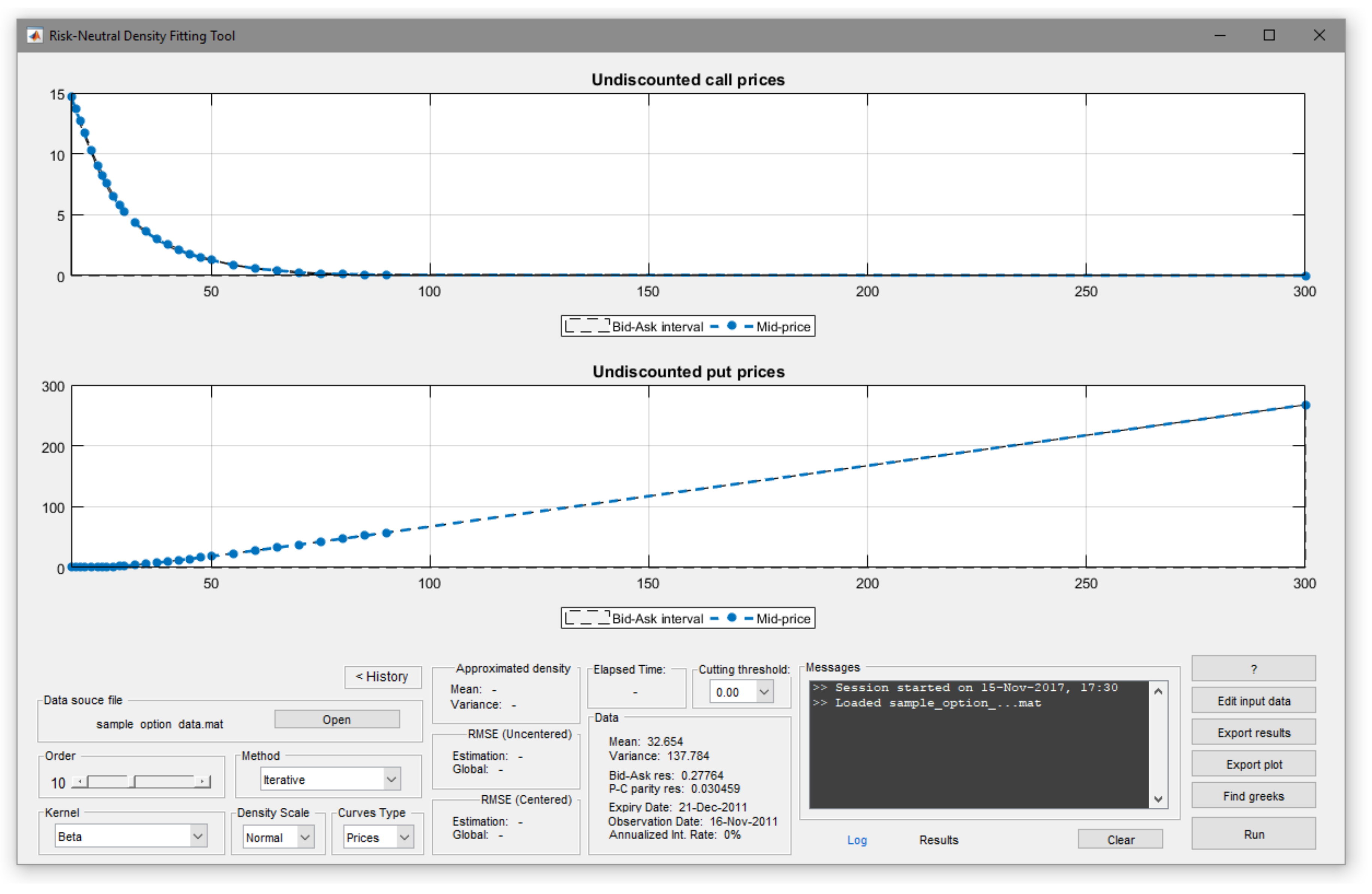
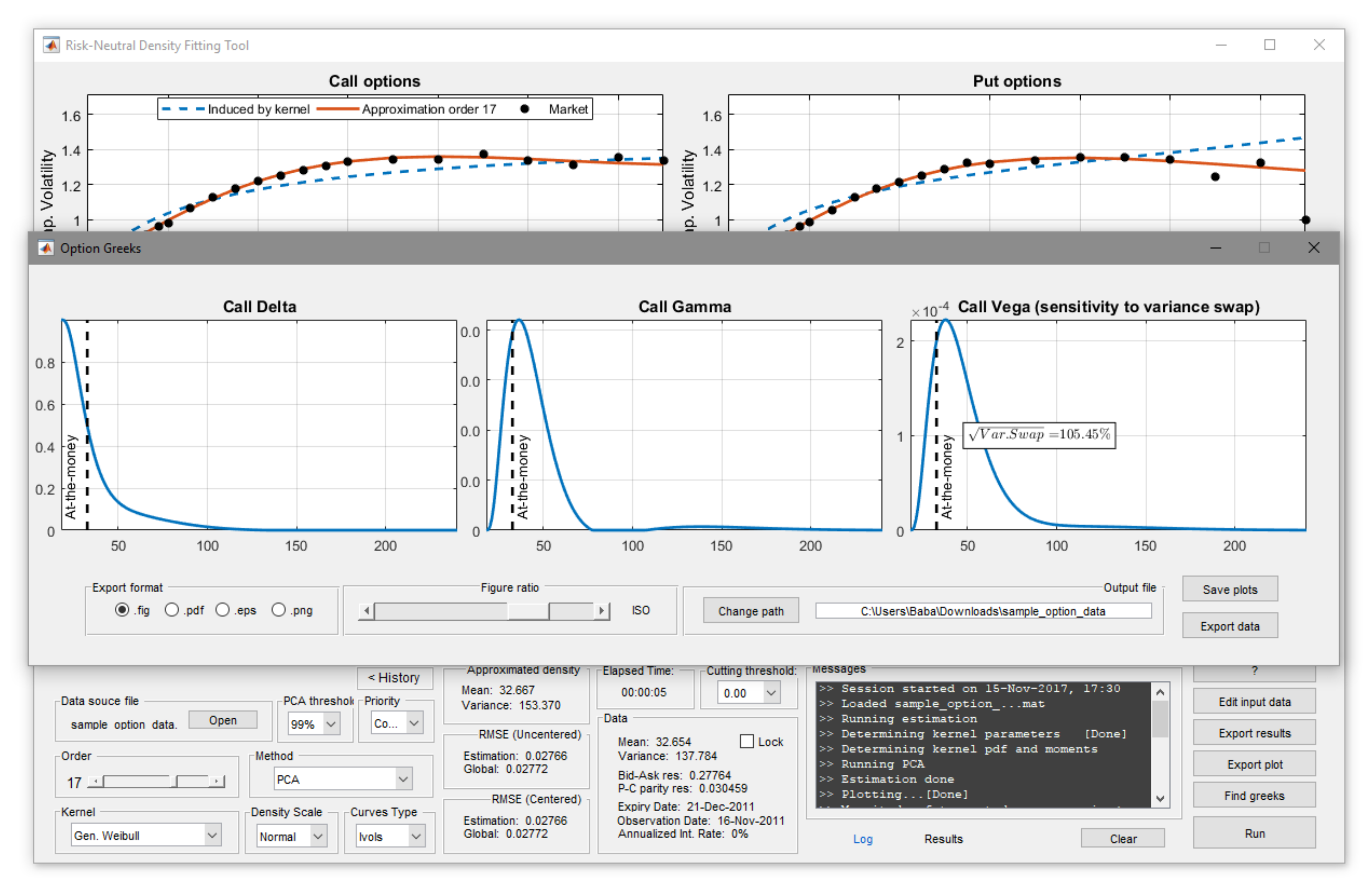
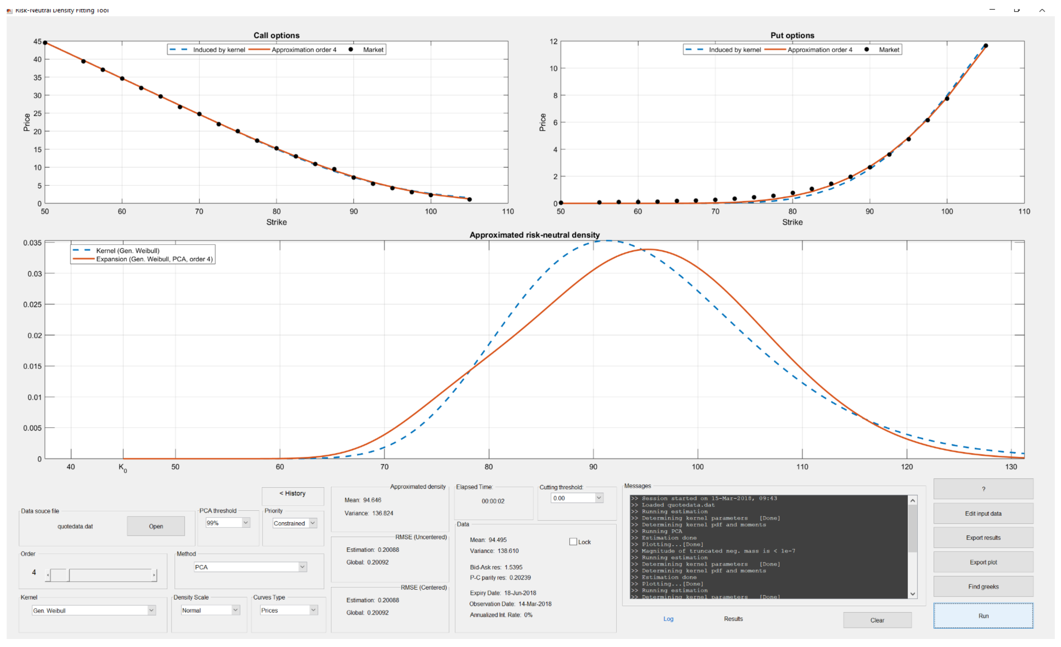
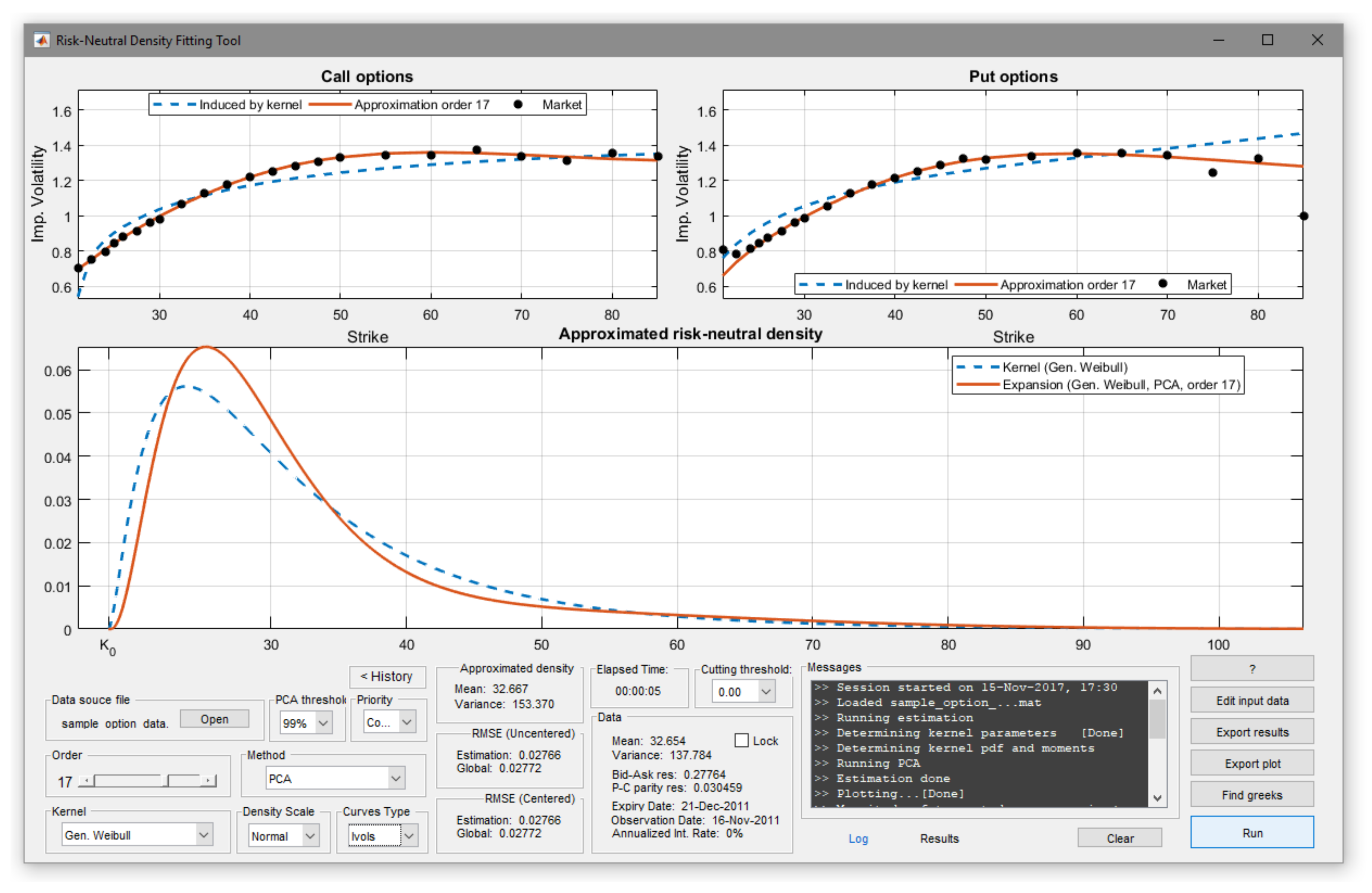
3. Using the App rndfittool

3.1. Package Overview

The app rndfittool provides a number of functions for fitting the RND from a set of option prices following the methodology outlined in Section 2. To make the tool easier to use for applied scientists, an interactive and user-friendly graphical user interface (GUI) has been implemented. The GUI can be used to load the option data, set and graphically inspect the tolerance on the mispricing associated with the observed option data, select the kernel density, run the polynomial expansion, plot the fitted density and the associated prices and implied volatilities, and finally export the results. The results of the analysis are shown directly in the interface and can be saved for later use. The GUI only requires the basic knowledge of MATLAB necessary to start MATLAB, to load the apps in MATLAB and to run the command starting the GUI. Within the interface, all options are visualized as buttons or drop-down menus. The interface has been tested on Linux and Windows 10 operating systems. The graphical user interface is started by downloading the automatic app installer of rndfittool from GitHub. rndfittool is then launched in MATLAB by clicking on the icon of the app. The MATLAB functions to generate rndfittool are open source, and they can be downloaded as a .zip file together with the app. Hence the user can have a complete overview on the MATLAB code behind the GUI, thus allowing her to modify and customize the algorithms. This feature gives the possibility to other members of the scientific community to operate extensions of the toolbox in the future.

The startup window of the GUI is shown in Figure 1. In the bottom-right corner are located the following buttons. Help: with detailed information on the functions, Edit input data: opens a new window to visually investigate the quality of the imported data and to initialize the coefficients of the kernel (see below), Export result: Allows for exporting the output of the fitting procedure in form of MATLAB functions, Export plot: Allows for exporting the output of the fitting procedure as plots, Find greeks: Extracts the delta, the gamma and the vega associated with the observed call prices. In the left part of the screen we find the button for the loading of the data (see the discussion below) and a number of bars and drop-down menus to select the type of fitting, the chosen kernel density and the type of plot required. The screen also contains a textual window with output messages from each operation.

3.2. General Data Structure

Input data are loaded by pressing “Open” in the main window. All data files must contain at least the following information: strike values, call prices, put prices. The standard compatible format for input data is a MAT-file with the structure described in

Table 1. Format of the input data.

Variable Name:	Size	Type	Description
K:	[M × 1 double]	Mandatory	Vector of strike values
call:	[M × 1 double]	Mandatory	Vector of observed call prices
put:	[M × 1 double]	Mandatory	Vector of observed put prices
m:	[2 × 1 double]	Mandatory	Vector with mean and variance of RND (can be set to [])
obsDate:	[1 × 6 int]	Optional	Observation date in numeric format ’yyyy mm dd’
expDate:	[1 × 6 int]	Optional	Expiry date in numeric format ’yyyy mm dd’
call_a:	[M × 1 double]	Optional	Vector of call ask prices
call_b:	[M × 1 double]	Optional	Vector of call bid prices
put_a:	[M × 1 double]	Optional	Vector of put ask prices
put_b:	[M × 1 double]	Optional	Vector of put bid prices

. Although, normally loading MATLAB-formatted data (.mat) is faster, input data can also be loaded from external sources (such as OptionMetrics and Chicago Board of Exchange, Cboe) in different formats and converted into compatible MAT-files at a later stage.

3.2.1. OptionMetrics

Option data must have .xls, .xlsx or .csv extension and formatted with all default options (e.g., date format) preset in the OptionMetrics download page. All columns related to mandatory variables must be contained in the dataset. Other field can be appended at any position of the spreadsheet. Options with several maturities and/or observation dates can be collected into the same file, in this case the user will be asked to make a choice. Website: Optionmetrics (2018).

3.2.2. Cboe

Data may be saved either into default .dat format available at Cboe Options Exchange (Cboe) website or may be pre-converted into .xls/.xlsx format. Data must contain all fields related to mandatory variables. Additional fields can be appended in any position of the dataset. Data for several maturities can be collected into the same file, in this case the user will be asked to choose a maturity when loading data. Website: Cboe (2018).

3.3. Analyzing Volatility Index (VIX) Options

Figure 2 reports the rndfittool window with the imported call and put options on VIX with 1-month maturity observed on 16 November 2011. The available strikes on the market are in the range between 18$ and 90$, but the range of the RND has been extended from 0 to 300. The prices associated with these strikes are not used in the fitting, but they determine the support of the RND. Once the option prices are loaded, it is possible to look at the quality of the dataset by clicking on the button Edit input data. Although being an optional procedure, this step is crucial, as it allows the user to perform a number of operations on the dataset, while maintaining the informational content of the original data. The new window for editing the input data is shown in Figure 3. The edit window allows to perform the following operations: Control for Concavity/Monotonicity to assess if the sample is characterized by extreme violations of the no arbitrage conditions across strike prices, assessing the magnitude of the deviations from the put-call parity, determine the boundaries for the domain of the density, and finally estimate the mean and variance of the RND by means of the non-parametric technique of Carr and Madan (1998). These are used as inputs for the initialization of the coefficients of the kernel. For VIX options, particular care should be given to the choice of the lower bound of the density, which should be placed reasonably far from 0 (kernel displacement) to improve the quality of the overall fit. For instance, in the present dataset put prices at 18$ are priced 3 cents, meaning that the RND between 0 and 16$ can be restricted to be 0 without loss of information, so that $K_0=16\$$. Notably, input data can always be exported into a compatible MAT-file, regardless of the source it was loaded from. This can be done by opening the data editor through “Edit input data” in the main window, and then selecting “Export input data”. At this point, the user is ready for the fitting of the RND, which is performed in the main window. The fitting requires to select among a number of options, which are illustrated below.

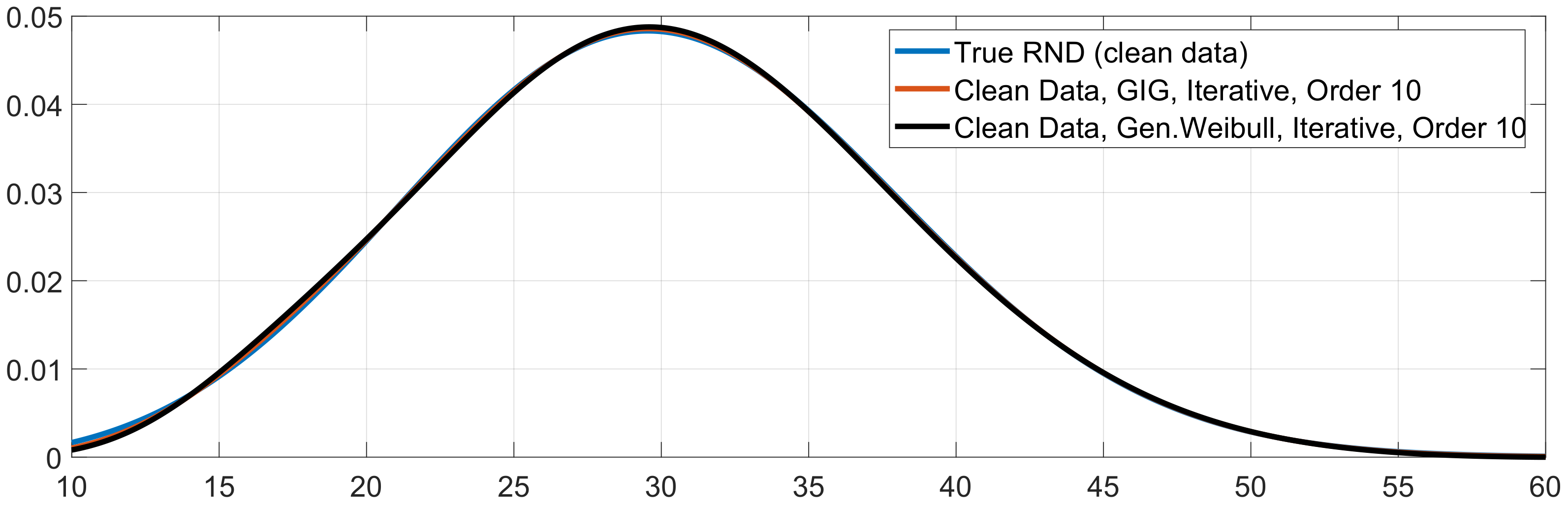
3.3.1. Choice of the Kernel Density

To guarantee a convergent expansion, the kernel $\varphi$ must decay at a slower rate than $f^2$, see Filipovic et al. (2013). Hence, an heavy-tailed kernel would make convergence easier to be met. On the other hand, the right tail of $\varphi$ must decay at an appropriate fast rate to ensure that in the limit for $n\to \infty$, the expansion converges exactly to the RND.

This is concerned with the so-called "completeness" of orthogonal polynomials, we refer to Filipovic et al. (2013) and Barletta et al. (2017) for further details. The following kernels are available to the user by default:

• Beta; $\varphi (x)\propto {(\frac{x}{c})}^{a-1}{(1-\frac{x}{c})}^{b-1},0\le x\le c$,
• Double beta; $\varphi (x)\propto \omega {(\frac{x}{c_1})}^{a_1-1}{(1-\frac{x}{c_1})}^{b_1-1}+(1-\omega ){(\frac{x}{c_2})}^{a_2-1}{(1-\frac{x}{c_2})}^{b_2-1},0\le x\le max(c_1,c_2)$,
• Gamma; $\varphi (x)\propto x^{\alpha -1}{e}^{-\beta x},x\ge 0$,
• Generalized Inverse Gaussian (GIG); $\varphi (x)\propto x^{\alpha -1}{e}^{-\frac{1}{2}\left(\beta x+\xi x^{-1}\right)},x\ge 0$,
• Generalized Weibull (GW); $\varphi (x)\propto x^{\alpha -1}{e}^{-\beta x^p},x\ge 0$,
• Lognormal; $\varphi (x)\propto \frac{1}{x}{e}^{-\frac{1}{2{\sigma }^2}{\left(log(x)-\mu \right)}^2},x\ge 0$,

We find the GIG and GW kernels to be the best choices for VIX options, while the double beta is better suited for option on the S&P 500 index (SPX) (without logarithmic transformation of the underlying). We emphasize that the code is structured in a way that any user can add custom kernels by adding a MAT-file in the folder named “kernels” containing the relevant information on $\varphi$. In general, the coefficients $a_k$ and $b_k$ given in (4) as well as the components of $\mathbf{X}$ given in (6) cannot be computed in closed-form. Hence, numerical quadrature techniques might be needed to evaluate the (incomplete) moments of $\varphi$. Notable exceptions are kernels such as the lognormal, the gamma and the generalized Weibull, for which the the above quantities can be computed in terms of special functions and are known in closed form. The MATLAB code is structured to deal with this issue as follows: first, the efficient recursive scheme outlined in Section 2 is used for the determination of the orthogonal polynomials; second, the user can include closed-form specifications for the (incomplete) moments upon adding a new kernel in the folder. Numerical quadrature algorithms are used only when this information is missing.

3.3.2. Choice of the Expansion Order

The expansion order is the number n in the expansion (2). In principle, increasing this number should also increase the accuracy of the approximation. However, in the practice, there are two factors that may prevent convergence:

• Theoretical issues: convergence conditions depend on the asymptotic behavior of $f^2/\varphi$. In particular, the convergence of (2) depends on assumptions relating the tail behavior of the RND to that of $\varphi$. These conditions might not be respected for any choice of the kernel and consequently the expansion leads to divergent results as n grows.
• Numerical issues: for large values of n high order polynomials are involved in the numerical computations, mainly of integrals and matrix inversion. Then computational issues may arise, depending on the estimation method being used and the kernel function adopted.

Optimal values of the expansion order are normally between 10 and 15 when using the PCA method on liquid options such as those on VIX. This is confirmed by the empirical analysis carried out in Barletta et al. (2017). On the contrary, when dealing with very illiquid and noisy options, such as those on individual stocks, then the number of expansion terms should be generally set to a low value.

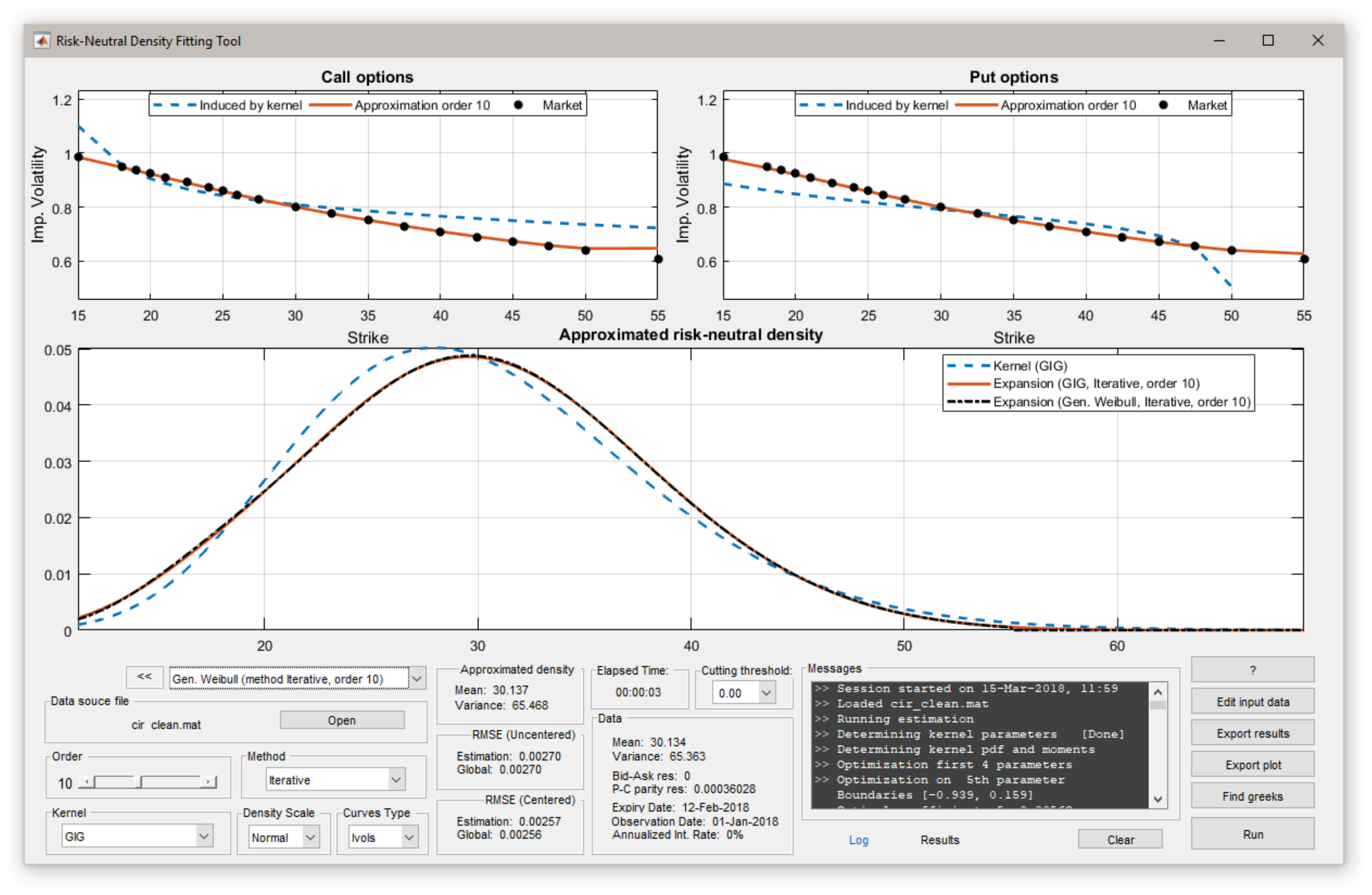
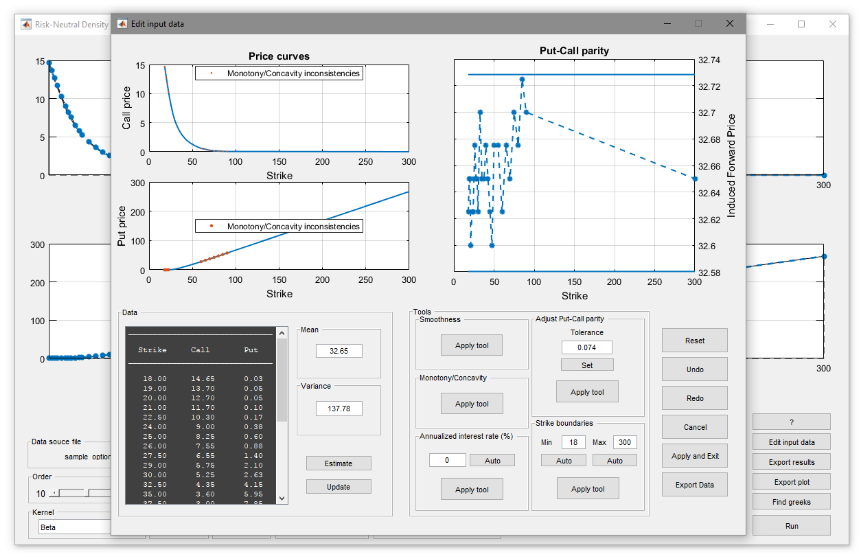
3.3.3. Fitting Methodology

There are three methods available to estimate the coefficients $c_1,\dots ,c_n$ of the expansion (2):

• Iterative: by this method a coefficient-by-coefficient estimation is performed and additional stability conditions can be imposed within the procedure. This is the most stable method and should not return divergent results even for high values of n. This method might be affected by issues related to overfitting and it performs well when the input data does not display inconsistencies or violations of no-arbitrage pricing, e.g., simulated data.
• Ordinary Least Squares (OLS): by this method the estimation is made by means of the ordinary least squares approach. This is the simplest but weakest method, from both an analytical and a statistical point of view, due to multicollinearity in the orthogonal polynomials. Indeed, expansions with order higher than 5 are unlikely to provide good results with this method.
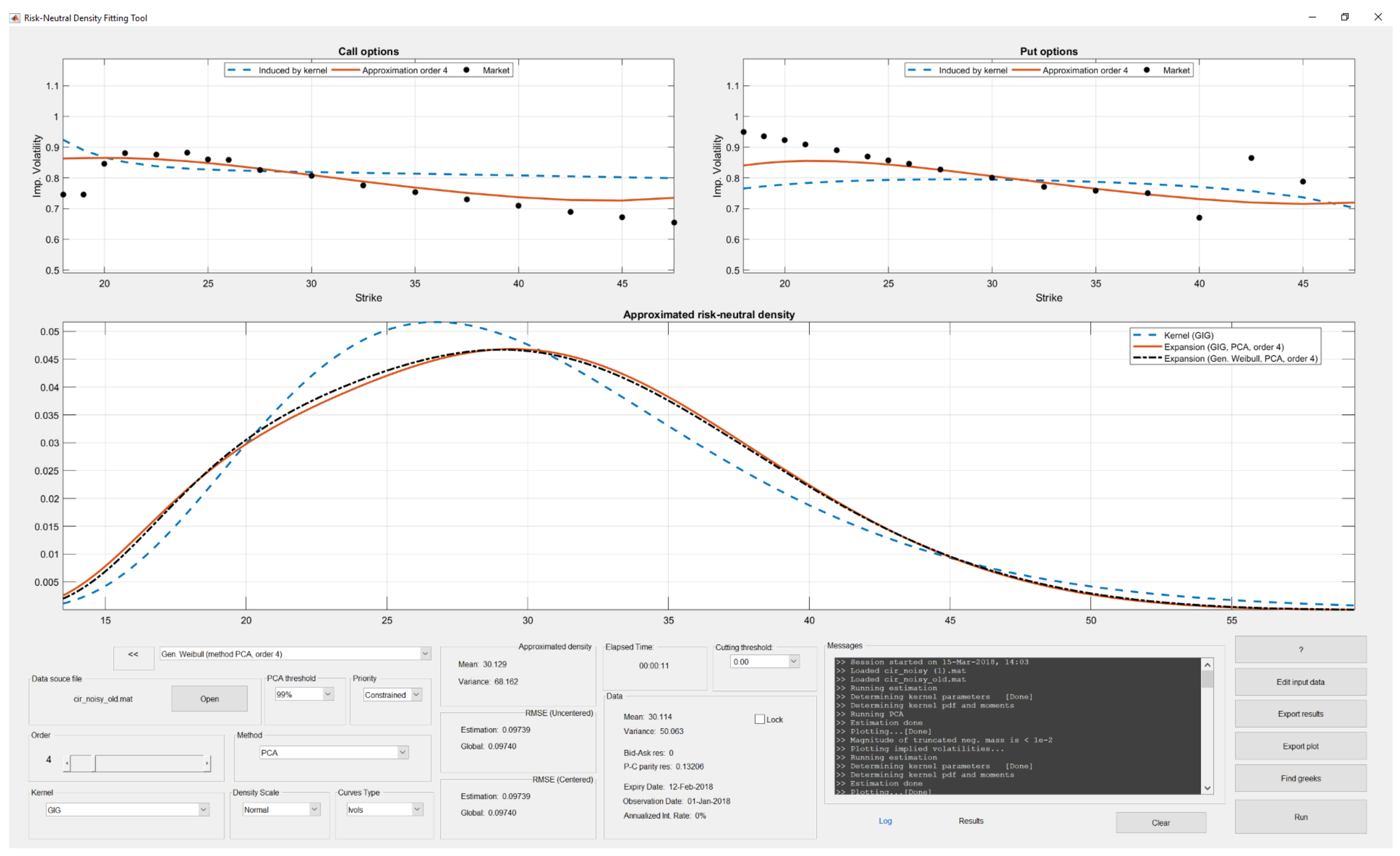
• PCA: This is the most robust method. The estimation of $c_1,\dots ,c_n$ is made by resorting to a linear combination of the expansion polynomials obtained by PCA. This method generally proves an efficient solution to both overfitting and multicollinearity. When the estimation is made on the real data, which typically exhibit some inconsistencies, the PCA method generally provides the best performance. Optionally, the PCA can be constrained to provide price residuals centered around 0.

Note that in all cases it is possible to exclude some data from the estimation without necessarily edit the input file. This can be done by setting the value displayed in the field named “Cutting threshold”. All pairs of call and put prices below the threshold are excluded from the estimation, together with the related strikes. A natural criterion for assessing the quality of the fitted curve is to compare the root-mean squared error (RMSE) of the residuals of the fitted model with that implied by the put-call parity (PCP) residuals, which is a measure of the noise in the original dataset. Indeed, under perfect market conditions and absence of arbitrage opportunities, the PCP residuals should be 0 across all strikes. If the RMSE of the estimation residuals lies significantly below the RMSE of the PCP, then we conclude that the estimated RND should be discarded due to overfitting. On the other hand, if the RMSE of the estimation residuals is much larger than that of PCP, the user has several options: a different choice of the kernel, an extension of the expansion order, or, ultimately, the exclusion of some of the option prices (typically in the tails) often associated with a lot of noise.

3.3.4. Output

Figure 4 reports the output window with the fitting of the VIX options.

The main plot reports the shape of the fitted RND (in red) and the kernel (in blue), thus highlighting the role of the estimated coefficients ${\widehat{c}}_1,\dots ,{\widehat{c}}_n$ as correction terms in the expansion (2). The top graph displays the fitting of the implied volatility curves for both call and put prices. It is important to stress that, although the estimation of the RND is performed on the option prices directly, the quality of the fit of the implied volatilities is remarkable. A drop-down menu allows the user to decide to plot the fitting of the implied volatilities, the fitting of the option prices or, alternatively, to display the estimation residuals. The output can be exported in two ways:

• Exporting graphs: by “Export plot” all plots displayed in the current window will be saved into three image files. Aspect ratio and extension of the exported images can be chosen by the user.
• Exporting all output as data: by “Export results” current results will be exported into a MAT-file with the structure outlined in

  Table 2. Output format.

  Variable Name:	Size	Description
  K:	[M × 1 double]	Vector of strike values
  obsCall:	[M × 1 double]	Vector of observed call prices
  obsPut:	[M × 1 double]	Vector of observed call prices
  c:	[1 × (n + 1) double]	Vector of estimated expansion coefficients
  kerPar:	[1 × P double]	Estimated coefficients of the kernel
  f:	function handle	RND as a MATLAB function handle
  kf:	function handle	Kernel density as a MATLAB function handle
  order:	[1 × 1 int]	Expansion order
  kernel:	[1 × D char]	Name of the Kernel density

  .

The estimated RND can be exported as a MATLAB function handle and used for extracting useful information for risk management such as the higher moments or quantiles like the VaR under the risk-neutral measure, see Aït-Sahalia and Lo (2000) and Barletta et al. (2017). Finally, based on the estimated RND, delta, gamma and vega hedge ratios can be computed non-parametrically following the methodology outlined in Barletta et al. (2018) and adopted for hedging purposes, see Figure 5.

3.3.5. Other Examples

The app rndfitool allows to fit the RND of any type of asset, as long as a strip of European options is available. As an additional example, we look at the European option prices for Microsoft (MSFT) available on Cboe on 14 March 2018 for contracts expiring on 18 June 2018 (approximately 3 months maturity). Figure 6 displays the output obtained with the generalized Weibull kernel with PCA expansion of order 4. The dataset originally contained $M=31$ strike prices in the range between 32.5 and 120. However, most of the put options in the range between 32.5 and 50 dollars were characterized by extremely large bid-ask spreads and the mid-quote was 1 or 2 cents. The options associated with these strike prices have been excluded from the analysis, and a lower bound for the option has been placed at $K_0=45$. The data are still extremely noise, with a bid-ask spread RMSE of 1.5 dollars and a PCP residuals of 20%. With such an high level of noise, the fitting of the RND is extremely challenging. To avoid over-fitting, we keep the number of expansion coefficient moderately low, $n=4$, and we use PCA. Also in this case, the fitting is remarkable and the generated RMSE on the prices matches the RMSE of the PCP residuals at 20%. This shows how the baseline structure given by the kernel helps in situation characterized by high levels of noise in the observed data.

To confirm the accuracy and robustness of the orthogonal polynomials to the noise on the option prices, we also display the results obtained on a set of option prices generated according to a known distribution. In particular, we have generated option prices from a modified version of the CIR model of Cox et al. (1985), which is consistent with VIX modeling, see Zhang and Zhu (2006). According to the CIR, the random variable Y has density

$$g(y)=C_1{y}^{\frac{k\zeta }{{\eta }^2}-\frac{1}{2}}{e}^{-\frac{2ky}{{\eta }^2(1-e^{-k\tau })}}{I}_{\frac{2k\zeta }{{\eta }^2}-1}(C_2\sqrt{y}),$$

(13)

where $C_1=\frac{2k}{{\eta }^2(1-e^{-k\tau })}$ and $C_2=2C_1\sqrt{e^{-k\tau }z}$, do not depend on the state variable s and $I_{\nu }$ denotes the modified Bessel function of first kind of order $\nu$. Finally, the true RND for the random variable of interest $X={(b+aY)}^{1/2}$ is a transformation of $g(y)$ as

$$f(x)=\frac{2}{a}x·g\left({\displaystyle \frac{x^2-b}{a}}\right).$$

(14)

Figure 7 reports the true RND and the fitted ones based on generated observations without noise.

Using either the GIG or the GW kernel, we obtain a perfect fit of the true RND, thus confirming the robustness of the choice of the kernel density. The algorithm adopted to retrieve the fitted density exploits the iterative method, which is sufficient when the data are free of no-arbitrage violations.

Figure 8 displays the output of the RND fitting obtained with rndfitool in this case. As expected, the put-call parity violations have basically zero variability and the small observed RMSE (0.03%) can be attributed to numerical errors. The figure illustrates the improvement in the fitting obtained by adjusting the kernel density by the polynomial expansions with both the GIG and the GW kernels. Notably, the matching of the implied-volatility curves obtained with the polynomial expansions is almost perfect in both cases.

Finally, we consider a setup characterized by noise on the observed prices. In particular, we contaminate the option prices with noise such that the RMSE on the put-call parity residuals is 13%. This level of noise is slightly below the extreme value observed on MSFT options (19%), while it is much larger than the one observed for more liquid options, such as VIX options (3%). Figure 9 shows that adopting the PCA to deal with noisy data not only reduces the risk of overfitting, but allows to retrieve an RND which displays approximately the same shape as the true RND shown in Figure 7 for both the GIG and the GW kernels. Notably, the RMSE on the price residuals is of the same order as the put-call parity residuals and it is approximately 10%.

4. Conclusions

The present paper demonstrates the use of the MATLAB app rndfittool for the estimation of the RND embedded in sets of European option prices. The package is built exploiting the MATLAB routines for GUI interfaces and thus provides a robust tool for analyzing option prices and extracting information relevant for risk management. The fitting methodology can be easily designed thanks to a highly configurable interface and the quality of the output can be easily assessed by analysis of the graphs or by comparison with the RMSE of the PCP. One of the biggest advantages, besides of being fast, is the flexible and at the same time intuitive specification framework. Notably, the set of available kernels can be extended by the user, simply by including new custom functions as explained in Section 3.3. For these reasons, we believe that rndfittool is a useful tool for both financial analysts and academic researchers, as well as a valid instrument for teaching purposes.

References

1. Ackerer, Damien, and Damir Filipović. 2017. Option Pricing with Orthogonal Polynomial Expansions. Technical Report. Ithaca: Cornell University Library. [Google Scholar]
2. Aït-Sahalia, Yacine, and Andrew W. Lo. 2000. Nonparametric risk management and implied risk aversion. Journal of Econometrics 94: 9–51. [Google Scholar] [CrossRef]
3. Alexander, Carol, and Leonardo M. Nogueira. 2007. Model-free hedge ratios and scale-invariant models. Journal of Banking & Finance 31: 1839–61. [Google Scholar]
4. Barletta, Andrea, and Elisa Nicolato. 2017. Orthogonal expansions for VIX options under affine jump diffusions. Forthcoming on Quantitative Finance. [Google Scholar] [CrossRef]
5. Barletta, Andrea, Paolo Santucci de Magistris, and David Sloth. 2018. It Only Takes a Few Moments to Hedge. Technical Report. Rochester: SSRN. [Google Scholar]
6. Barletta, Andrea, Paolo Santucci de Magistris, and Francesco Violante. 2017. A Non-Structural Investigation of VIX Risk Neutral Density. Technical Report. Rochester: SSRN. [Google Scholar]
7. Bates, David S. 2005. Hedging the smirk. Finance Research Letters 2: 195–200. [Google Scholar] [CrossRef]
8. Breeden, Douglas T., and Robert H. Litzenberger. 1978. Prices of state-contingent claims implicit in option prices. The Journal of Business 51: 621–51. [Google Scholar] [CrossRef]
9. Carr, Peter, and Dilip Madan. 1998. Towards a theory of volatility trading. In Volatility: New Estimation Techniques for Pricing Derivatives. London: Risk Books, pp. 417–27. [Google Scholar]
10. Cboe. 2018. Available online: http://www.cboe.com/ (accessed on 14 March 2018).
11. Coutant, Sophie, Eric Jondeau, and Michael Rockinger. 2001. Reading PIBOR futures options smiles: The 1997 snap election. Journal of Banking & Finance 25: 1957–87. [Google Scholar]
12. Cox, John, Jonathan E. Ingersoll, and Stephen A. Ross. 1985. A theory of the term structure of interest rates. Econometrica 53: 385–408. [Google Scholar] [CrossRef]
13. Drimus, Gabriel G., Ciprian Necula, Anastasiia Sokko, and Walter Farkas. 2013. Closed Form Option Pricing under Generalized Hermite Expansions. Technical Report. Farkas: SSRN. [Google Scholar]
14. Filipovic, Damir, Eberhard Mayerhofer, and Paul Schneider. 2013. Density approximations for multivariate affine jump-diffusion processes. Journal of Econometrics 176: 93–111. [Google Scholar] [CrossRef]
15. Jarrow, Robert, and Andrew Rudd. 1982. Approximate option valuation for arbitrary stochastic processes. Journal of Financial Economics 10: 347–69. [Google Scholar] [CrossRef]
16. Madan, Dilip B., and Frank Milne. 1994. Contingent claims valued and hedged by pricing and investing in a basis. Mathematical Finance 4: 223–45. [Google Scholar] [CrossRef]
17. Mencía, Javier, and Enrique Sentana. 2017. Volatility-related exchange traded assets: An econometric investigation. Journal of Business & Economic Statistics 0: 1–16. [Google Scholar]
18. Optionmetrics. 2018. Available online: http://www.optionmetrics.com/ (accessed on 23 January 2018).
19. Xiu, Dacheng. 2014. Hermite polynomial based expansion of European option prices. Journal of Econometrics 179: 158–77. [Google Scholar] [CrossRef]
20. Zhang, Jin E., and Yingzi Zhu. 2006. VIX futures. Journal of Futures Markets 26: 521–31. [Google Scholar] [CrossRef]
Figure 1. Startup window of the rndfittool graphical user interface (GUI).
Risks 06 00028 g001
Figure 2. The imported dataset of volatility index (VIX) options observed on 16 November 2011.
Risks 06 00028 g002
Figure 3. Edit window for VIX options on 16 November 2011.
Risks 06 00028 g003
Figure 4. Risk-neutral density (RND) obtained with a Generalized Inverse Gaussian (GIG) kernel and expansion order n = 18 and 5 principal component analysis (PCA) components with a treshold of 99%.
Risks 06 00028 g004
Figure 5. Greeks obtained with a GIG kernel and expansion order n = 18 with 5 PCA terms.
Risks 06 00028 g005
Figure 6. RNDs obtained from Microsoft (MSFT) options observed on 14 March 2018 and with maturity 18 June 2018. Source Cboe.
Risks 06 00028 g006
Figure 7. True and fitted RNDs based on the modified CIR density in (14). The data is generated with parameters k = 1.71 , ζ = 0.097 , η = 0.577 and τ = 30 / 365 . The fitted RNDs are obtained with a GIG and GW kernels for n = 10 .
Risks 06 00028 g007
Figure 8. The data is generated by a CIR density with parameters k = 1.71 , ζ = 0.097 , η = 0.577 and τ = 30 / 365 .
Risks 06 00028 g008
Figure 9. rndfittol output with the kernel density of the GIG, the fitted RNDs (with both GIG and GW) and the implied-volatility curve when observed option prices are contaminated by noise. The red line is the fitted RND obtained with the GIG kernel and the black line is the fitted RND obtained with GW kernel. In both cases, we consider PCA with expansion order n = 4 .
Risks 06 00028 g009