Target Matrix Estimators in Risk-Based Portfolios

Abstract

Portfolio weights solely based on risk avoid estimation errors from the sample mean, but they are still affected from the misspecification in the sample covariance matrix. To solve this problem, we shrink the covariance matrix towards the Identity, the Variance Identity, the Single-index model, the Common Covariance, the Constant Correlation, and the Exponential Weighted Moving Average target matrices. Using an extensive Monte Carlo simulation, we offer a comparative study of these target estimators, testing their ability in reproducing the true portfolio weights. We control for the dataset dimensionality and the shrinkage intensity in the Minimum Variance (MV), Inverse Volatility (IV), Equal-Risk-Contribution (ERC), and Maximum Diversification (MD) portfolios. We find out that the Identity and Variance Identity have very good statistical properties, also being well conditioned in high-dimensional datasets. In addition, these two models are the best target towards which to shrink: they minimise the misspecification in risk-based portfolio weights, generating estimates very close to the population values. Overall, shrinking the sample covariance matrix helps to reduce weight misspecification, especially in the Minimum Variance and the Maximum Diversification portfolios. The Inverse Volatility and the Equal-Risk-Contribution portfolios are less sensitive to covariance misspecification and so benefit less from shrinkage.

1. Introduction

The seminal contributions of Markowitz (1952, 1956) laid the foundations for his well-known portfolio building technique. Albeit elegant in its formulation and easy to be implemented in real-world applications, the Markowitz model relies on securities returns sample mean and sample covariance as inputs to estimate the optimal allocation. However, there is a large consensus on the fact that sample estimators perpetuate large estimation errors; this directly affects portfolio weights that often exhibit extreme values, fluctuating over time with very poor performance out-of-sample (De Miguel et al. 2009).

This problem has been tackled from different perspectives: Jorion (1986) and Michaud (1989) suggested Bayesian alternatives to the sample estimators; Jagannathan and Ma (2003) added constraints to the Markowitz model limiting the estimation error; Black and Litterman (1992) derived an alternative portfolio construction technique exclusively based on the covariance matrix among asset returns, avoiding estimating the mean value for each security and converging to the Markowitz Minimum Variance portfolio with no short-sales. This latter technique is supported by results in Merton (1980) and Chopra and Ziemba (1993), who clearly demonstrated how the mean estimation process can lead to more severe distortions than those in the case of the covariance matrix.

Following this perspective, estimation error can be reduced by considering risk-based portfolios: findings suggest they have good out-of-sample performance without much turnover (De Miguel et al. 2009). There is a recent research strand focused on deriving risk-based portfolios other than the Minimum Variance one. In this context, Qian (2006) designed a way to select assets by assigning to each of them the same contribution to the overall portfolio risk; Choueifaty and Coignard (2008) proposed a portfolio where diversification is the key criterion in asset selection; Maillard et al. (2010) offered a novel portfolio construction technique where weights perpetuate an equal risk contribution while maximising diversification. These portfolios are largely popular among practitioners1: they highlight the importance of diversification, risk budgeting; moreover, they put risk management in a central role, offering a low computational burden to estimate weights. They are perceived as “robust” models since they do not require the explicit estimation of the mean. Unfortunately, limiting the estimation error in this way poses additional problems related to the ill-conditioning of the covariance matrix that occurs when the number of securities becomes sensitively greater than the number of observations. In this case, the sample eigenvalues become more dispersed than the population ones (Marčenko and Pastur 1967), and the sample covariance matrix directly affects weight estimation. This means that for a high-dimensional dataset, the sample covariance matrix is not a reliable estimator.

To reduce misspecification effects on portfolio weights, more sophisticated estimators than the sample covariance have been proposed, for example the Bayes-Stein shrinkage technique (James and Stein 1961), henceforth shrinkage stems for its practical implementation and related portfolio performance. This technique reduces the misspecification in the sample covariance matrix by shrinking it towards an alternative estimator. Here, the problem is to select a convenient target estimator as well as to find the optimal intensity at which to shrink towards the sample covariance matrix. The latter is usually derived by minimising a predefined loss function to obtain the minimum distance between the true and the shrunk covariance matrices (Ledoit and Wolf 2003). A comprehensive overview on shrinkage intensity parameters can be found in (De Miguel et al. 2013), where the authors proposed an alternative way of deriving the optimal intensity based on the smoothed bootstrap approach. On the other hand, the target matrix is often selected among the class of structured covariance estimators (Briner and Connor 2008), especially because the matrix which shrinks is the sample one. As noted in (Candelon et al. 2012), the sample covariance matrix is the Maximum Likelihood Estimator (MLE) under the Normality of asset returns, hence it lets the data speak without imposing any structure. This naturally suggests it might be pulled towards a more structured alternative. Dealing with financial data, the shrinkage literature proposes six different models for the target matrix: the Single-Index market model (Ledoit and Wolf 2003; Briner and Connor 2008; Candelon et al. 2012; Ardia et al. 2017); the Identity matrix (Ledoit and Wolf 2004a; Candelon et al. 2012); the Variance Identity matrix (Ledoit and Wolf 2004a); the Scaled Identity matrix (De Miguel et al. 2013); the Constant Correlation model (Ledoit and Wolf 2004b) and (Pantaleo et al. 2011); the Common Covariance (Pantaleo et al. 2011). All these targets belong to the class of more structured covariance estimators than the sample one, thus implying the latter is the matrix to shrink.

Despite the great improvements in portfolio weight estimation under the Markowitz portfolio building framework, the shrinkage technique has only been applied in one work involving risk-based portfolios: that of Ardia et al. (2017), who comprehensively described the impacts of variance and covariance misspecifications in risk-portfolio weights. Ardia et al. (2017) tested four alternative covariance estimators to reduce weight misspecification; among those, only one refers to shrinkage as in (Ledoit and Wolf 2003), leaving room open for further research. In our work, we contribute to the existing literature, filling this gap and offering a comprehensive overview of shrinkage in risk-based portfolios. In particular, we study the effect of six target matrix estimators on the weights of four risk-based portfolios. To achieve this goal, we provide an extensive Monte Carlo simulation aimed at (1) assessing estimators’ statistical properties and similarity with the true target matrix; (2) addressing the problem of how the selection of a specific target estimator affects the portfolio weights. We find out that the Identity and Variance Identity hold the best statistical properties, being well conditioned even in a high-dimensional dataset. These two estimators also represent the more efficient target matrices towards which to shrink the sample one. In fact, portfolio weight derived shrinking towards the Identity and Variance Identity minimise the distance from their true counterparts, especially in the case of Minimum Variance and Maximum Diversification portfolios.

The rest of the paper is organised as follows. Section 2 introduces the risk-based portfolios employed in the study. Section 3 illustrates the shrinkage estimator, the moves to the six target matrix estimators and provides useful insights into misspecification when shrinkage is applied to risk-based portfolios. In Section 4, we run an extensive Monte Carlo analysis for describing how changes in the target matrix affect risk-based portfolio weights. Section 5 concludes.

2. Risk-Based Portfolios

Risk-based portfolios are particularly appealing since they rely only on the estimation of a proper measure of risk, i.e., the covariance matrix between asset returns. Assume an investment universe made by $p$ assets:

$$X= ({\mathit{x}}_1,\dots ,{\mathit{x}}_p)$$

(1)

is a $n\times p$ containing a history of $n$ log-returns for the i-th asset, where $i=1,\dots ,p$. The covariance matrix among asset log-returns is the symmetric square matrix $\mathrm{\Sigma }$2 of dimension $p\times p$, and the unknown optimal weights form the vector $\mathit{\omega }$ of dimension $p\times 1$. Our working framework assumes to consider four risk-based portfolios: the Minimum Variance (MV), the Inverse Volatility (IV), the Equal-Risk-Contribution (ERC), and the Maximum Diversification (MD) upon two constraints; no short-selling ($\mathit{\omega }\in {\Re }_{+}^p$) and full allocation of the available wealth (${\mathit{\omega }}^{\prime }{\mathbf{1}}_p=1$, where ${\mathbf{1}}_p$ is the vector of ones of length $p$).

The Minimum Variance portfolio (Markowitz 1952) derives the optimal portfolio weights by solving this minimization problem with respect to $\mathit{\omega }$:

$${\mathit{\omega }}_{MV}\equiv \underset{\mathit{\omega }}{\mathrm{argmin}}\{{\mathit{\omega }}^{\prime }\mathrm{\Sigma }\mathit{\omega } | \mathit{\omega }\in {\Re }_{+}^p,{\mathit{\omega }}^{\prime }{\mathbf{1}}_p=1\}$$

(2)

where ${\mathit{\omega }}^{\prime }\mathrm{\Sigma }\mathit{\omega }$ is the portfolio variance.

In the Inverse Volatility portfolio, also known as the equal-risk-budget portfolio (Leote de Carvalho et al. 2012), a closed form solution is available. Each element of the vector $\mathit{\omega }$ is given by the inverse of the i-th asset variance (denoted by ${\mathrm{\Sigma }}_{i,i}^{-1}$) divided by the inverse of the sum of all asset variances:

$${\mathit{\omega }}_{IV}\equiv {\left(\frac{{{\displaystyle \sum }}_{1,1}^{-1}}{{{\displaystyle \sum }}_{i=1}^p{{\displaystyle \sum }}_{i,i}^{-1}},\dots ,\frac{{{\displaystyle \sum }}_{p,p}^{-1}}{{{\displaystyle \sum }}_{i=1}^p{{\displaystyle \sum }}_{i,i}^{-1}}\right)}^{\prime }$$

(3)

In the Equal-Risk-Contribution portfolio, as the name suggests, the optimal weights are calculated by assigning to each asset the same contribution to the whole portfolio volatility, thus originating a minimization procedure to be solved with respect to $\mathit{\omega }$:

$${\mathit{\omega }}_{ERC}\equiv \underset{\mathit{\omega }}{\mathrm{argmin}}\{{\displaystyle \sum }_{i=1}^p{(\%{RC}_i-\frac{1}{p})}^2|\mathit{\omega }\in {\Re }_{+}^p,{\mathit{\omega }}^{\prime }{\mathbf{1}}_p=1\}$$

(4)

Here, $\%R{C}_i\equiv \frac{{\mathit{\omega }}_{i}co{v}_{i,\pi }}{\sqrt{{\mathit{\omega }}^{\prime }\mathrm{\Sigma }\mathit{\omega }}}$ is the percentage risk contribution for the i-th asset, $\sqrt{{\mathit{\omega }}^{\prime }\mathrm{\Sigma }\mathit{\omega }}$ is the portfolio volatility as earlier defined, and ${\mathit{\omega }}_{i}co{v}_{i,\pi }$ provides a measure of the covariance of the i-th exposure to the total portfolio $\pi$, weighted by the corresponding ${\mathit{\omega }}_i$.

Turning to the Maximum Diversification, as in Choueifaty and Coignard (2008) we preliminary define $DR\left(\mathit{\omega }\right)$ as the portfolio’s diversification ratio:

$$DR\left(\mathit{\omega }\right)\equiv \frac{{\mathit{\omega }}^{\prime }\sqrt{diag\left(\mathrm{\Sigma }\right)}}{\sqrt{{\mathit{\omega }}^{\prime }\mathrm{\Sigma }\mathit{\omega }}}$$

where $diag\left(\mathrm{\Sigma }\right)$ is a $p\times 1$ vector which takes all the asset variances ${\mathrm{\Sigma }}_{i,i}$ and ${\mathit{\omega }}^{\prime }\sqrt{diag\left(\mathrm{\Sigma }\right)}$ is the weighted average volatility. By construction, it is $DR\left(\mathit{\omega }\right)\ge 1$, since the portfolio volatility is sub-additive (Ardia et al. 2017). Hence, the optimal allocation is the one with the highest DR:

$${\mathit{\omega }}_{MD}\equiv \underset{\mathit{\omega }}{\mathrm{argmax}}\{DR\left(\mathit{\omega }\right)| \mathit{\omega }\in {\Re }_{+}^p,{\mathit{\omega }}^{\prime }{\mathbf{1}}_p=1\}.$$

(5)

3. Shrinkage Estimator

The shrinkage technique relies upon three ingredients: the starting covariance matrix to shrink, the target matrix towards which the former is shrunk, and the shrinkage intensity, or roughly speaking the strength at which the starting matrix must be shrunk.

In financial applications, the starting matrix which is to shrink is always the sample covariance matrix. This is a very convenient choice that helps in the selection of a proper shrinkage target: being the sample covariance a model-free estimator that completely reflects the relationships among data3, it becomes natural to select a target in the class of more structured covariance estimators (Briner and Connor 2008). In addition, this strategy allows direct control over the trade-off between estimation error and model error in the resulting shrinkage estimates. In fact, the sample covariance matrix is usually affected by a large amount of estimation error. This is reduced when shrinking towards a structured target which minimizes the sampling error at the cost of adding some misspecification by imposing a specific model. At this point, the shrinkage intensity is crucial because it must be set in such a way to minimize both errors.

To define the shrinkage estimator, we start from the definition of sample covariance matrix $S$. Recalling Equation (1), $S$ is given by

$$S= \frac{1}{n-1}{X}^{\prime \left(I_n-\frac{1}{n}{\mathbf{1}}_n{\mathbf{1}}_n^{\prime }\right)}X,$$

(6)

where $I_n$ denotes the $n\times n$ identity matrix and ${\mathbf{1}}_n$ is the ones column vector of length $n$. The shrinkage methodology enhances the sample covariance matrix estimation by shrinking $S$ towards a specific target matrix $T$:

$${\mathrm{\Sigma }}_s= \delta T+\left(1-\delta \right)S$$

(7)

where ${\mathrm{\Sigma }}_s$ is the shrinkage estimator; $\delta$ the shrinkage parameter and $T$ the target matrix. In this work, we focus on the problem of selecting the target matrix. After a review of the literature on target matrices, in the following rows we present the target estimators considered in this study and we assess through a numerical illustration the impact of misspecification in the target matrix for the considered risk-based portfolios.

3.1. Target Matrix Literature Review

The target matrix should fit a desirable number of requirements: First, it should be structured much enough to lower the estimation error of the sample covariance matrix while not bringing too much error from model selection. Second, it should reflect the important features of the true covariance matrix (Ledoit and Wolf 2004b). The crucial question is: how much structure should we impose to fill in the requirements?

Table 1. Literature review of target matrices. “SCVm” = sample covariance matrix. “N.A.” = not available. “GMVP” = Global Minimum Variance Portfolio.

Reference	Matrix to Shrink	Target Matrix	Shrinkage Intensity	Portfolio Selection Rule	Research Question
(Ledoit and Wolf 2003)	SCVm	Market Model and Variance Identity	Risk-function minimisation	Classical Markowitz problem	Portfolio Performance comparison
(Ledoit and Wolf 2004a)	SCVm	Identity	Risk-function minimisation	N.A.	Theoretical paper to gauge the shrinkage asymptotic properties
(Ledoit and Wolf 2004b)	SCVm	Constant Correlation Model	Optimal shrinkage constant	Classical Markowitz problem	Portfolio Performance comparison
(Briner and Connor 2008)	Demeaned SCVm	Market Model	Same as (Ledoit and Wolf 2004b)	N.A.	Analysis of the trade-off estimation error and model specification error
(Pantaleo et al. 2011)	SCVm	Market Model, Common Covariance and Constant Correlation Model	Unbiased estimator of (Schäfer and Strimmer 2005)	Classical Markowitz problem	Portfolio Performance comparison
(Candelon et al. 2012)	SCVm	Market Model and Identity	Same as (Ledoit and Wolf 2003, 2004b)	Black-Litterman GMVP	Portfolio Performance comparison
(De Miguel et al. 2013)	SCVm	Scaled Identity	Expected quadratic loss and bootstrapping approach	Classical Markowitz problem	Comprehensive investigation of shrinkage estimators
(Ardia et al. 2017)	SCVm	Market Model	Same as (Ledoit and Wolf 2003)	Risk-based portfolios	Theoretical paper to assess effect on risk-based weights

shows the target matrices employed so far in the literature, summarising information about the formula for the shrinkage intensity, the wealth allocation rule, and the addressed research question. Not surprisingly, all the papers shrink the sample covariance matrix. What surprises is that only six target matrices have been examined: the one relying on the Single-Index market model, the Identity matrix, the Scaled Identity, and the Variance Identity, the Constant Correlation model and the Common Covariance model. Previously, four were proposed by Ledoit and Wolf in separate works (Ledoit and Wolf 2003, 2004a, 2004b) and were again proposed in subsequent works, while the Common Covariance appears only in (Pantaleo et al. 2011) and the Scaled Identity only in (De Miguel et al. 2013).

In Table 1, papers have been listed taking into account their contribution to the literature as regards the adoption of a novel target matrix estimator, the re-examination of a previously proposed target, and the comparison among different estimators. Ledoit and Wolf popularised the shrinkage methodology in portfolio selection: in Ledoit and Wolf (2003), they were also the first to compare the effects of shrinking towards different targets in portfolio performance. Shrinking towards the Variance Identity and shrinking towards the Market Model are two out of the eight estimators for the covariance matrix compared with respect to the reduction of estimation error in portfolio weights. They found significant improvements in portfolio performance when shrinking towards the Market Model. Briner and Connor (2008) well described the importance of selecting the target matrix among the class of structured covariance estimators, hence proposing to shrink the asset covariance matrix of demeaned returns towards the Market model as in Ledoit and Wolf (2003). Candelon et al. (2012) compared the effect of double shrinking the sample covariance either towards the Market Model and the Identity, finding that both estimators carry on similar out-of-sample performances. De Miguel et al. (2013) compared the effects of different shrinkage estimators on portfolio performance, highlighting the importance of the shrinkage intensity parameter and proposing a scaled version of the Identity Matrix as a target. Another important comparison among target matrices is that of Pantaleo et al. (2011), who compared the Market and Constant Correlation models as in Ledoit and Wolf (2003, 2004b) with the Common Covariance of Schäfer and Strimmer (2005) implemented as target matrix for the first time in finance. The authors assessed the effects on portfolio performances while controlling for the dimensionality of the dataset, finding that the Common Covariance should not be used when the number of observations is less than the number of assets. Lastly, Ardia et al. (2017) is the only work to implement shrinkage in risk-based portfolios. They shrunk the sample covariance matrix as in Ledoit and Wolf (2003), finding that the Minimum Variance and the Maximum Diversification portfolios are the most affected from covariance misspecification, hence they benefit the most from the shrinkage technique.

3.2. Estimators for the Target Matrix

We consider six estimators for the target matrix: the Identity and the Variance Identity matrix, the Single-index, the Common Covariance, the Constant Correlation and the Exponential Weighted Moving Average (EWMA) models. They are all structured estimators, in the sense that the number of parameters to be estimated is far less the $\frac{1}{2}p\left(p+1\right)$ required in the sample covariance case. Compared with the literature, we take into account all the previous target estimators,4 adding to the analysis the EWMA: this estimator well addresses the problem of serial correlation and heteroskedasticity in asset returns.

The identity is a matrix with ones on the diagonal and zeros elsewhere. Choosing the Identity as the target is justified by the fact that is shows good statistical properties: it is always well conditioned and hence invertible (Ledoit and Wolf 2003). Besides the identity, we also consider a multiple of the identity, named the Identity Variance. This is given by:

$$T_{VId}\equiv I_{p}diag\left(S\right)I_p,$$

(8)

where $diag\left(S\right)$ is the main diagonal of the sample covariance matrix (hence the assets variances) and $I_p$ the identity matrix of dimension p.

The Single Index Model (Sharpe 1963) assumes that the returns ${\mathit{r}}_t$ can be described by a one-factor model, resembling the impact of the whole market:

$$\begin{gathered} {\mathit{r}}_t=\mathit{\alpha }+\mathit{\beta }{r}_{mkt}+{\epsilon }_t, \\ \mathrm{with} t=1,\dots ,n, \end{gathered}$$

where $r_{mkt}$ is the overall market returns; $\mathit{\beta }$ is the vector of factor estimates for each asset; $\mathit{\alpha }$ is the market mispricing, and ${\epsilon }_t$ the model error. The Single-Index market model represents a practical way of reducing the dimension of the problem, measuring how much each asset is affected by the market factor. The model implies the covariance structure among asset returns is given by:

$$T_{si}\equiv s_{mkt}^2\mathit{\beta }{\mathit{\beta }}^{\prime }+\mathsf{\Omega },$$

(9)

where $s_{mkt}^2$ is the sample variance of asset returns; $\mathit{\beta }$ is the vector of beta estimates and $\mathsf{\Omega }$ contains the residual variance estimates.

The Common Covariance model is aimed at minimizing the heterogeneity of assets variances and covariances by averaging both of them (Pantaleo et al. 2011). Let ${\mathrm{var}}_{ij,i=j}$ and ${\mathrm{covar}}_{ij, i\ne j}$ being the variances and covariances of the sample covariance matrix, respectively, their averages are given by:

$$\overline{\mathrm{var}}=\frac{1}{p}{\displaystyle \sum }_{k=1}^p{\mathrm{var}}_{k,i=j};$$

$$\overline{\mathrm{covar}}=\frac{1}{p\left(p-1\right)/2}{{\displaystyle \sum }}_{k=1}^{p\left(p-1\right)/2}{\mathrm{covar}}_{k, i\ne j};$$

where $p$ is the number of securities. The resulting target matrix $T_{cv}$ has its diagonal elements all equal to the average of the sample covariance, while non-diagonal elements are all equal to the average of sample covariances.

In the Constant Correlation model the main diagonal is filled with sample variances, and elsewhere a constant covariance parameter which is equal for all assets. The matrix can be written according to the following decomposition:

$$T_{cc}\equiv P diag\left(S\right)P,$$

(10)

where $P$ is the lower triangular matrix filled with the constant correlation parameter $\overline{\rho }=\frac{1}{p\left(p-1\right)/2}{\displaystyle \sum }_{i=1}^p{\rho }_{ij}$ for $i<j$ and ones in the main diagonal. Here, $diag\left(S\right)$ represents the main diagonal of the sample covariance matrix.

The EWMA model (J. P. Morgan and Reuters Ltd. 1996) was introduced by JP Morgan’s research team to provide an easy but consistent way to assess portfolio covariance. RiskMetrics EWMA considers the variances and covariance driven by an Integrated GARCH process:

$$T_{\mathrm{EWMA},t}\equiv X^{\prime }X+\lambda T_{\mathrm{EWMA},t-1},$$

(11)

with $T_{\mathrm{EWMA},0}= I_p$ $T_{\mathrm{EWMA},t-1}$ is the target matrix at time $t-1$ and $\lambda$ is the smoothing parameter: the higher $\lambda$, the higher the persistence in the variance.

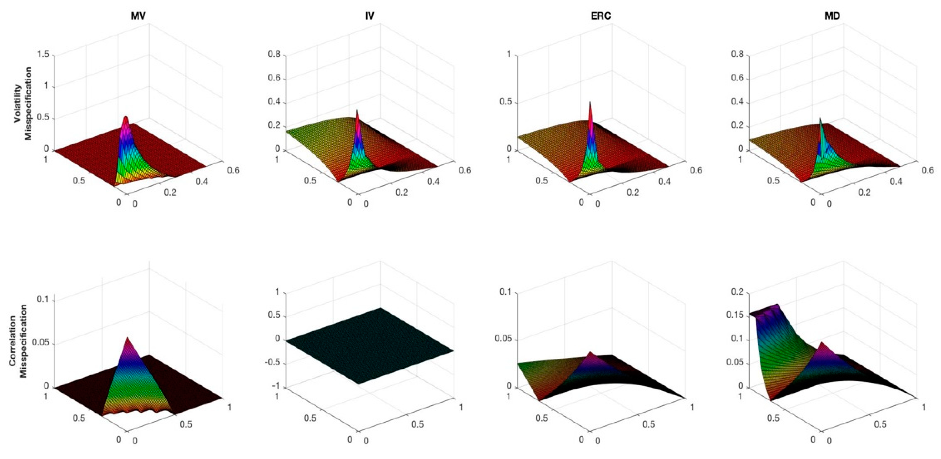
3.3. The Impact of Misspecification in the Target Matrix

We are now going to show to which extent risk-based portfolios can be affected by misspecification in the target matrix. To do so, we provide a numerical illustration, merely inspired by the one in Ardia et al. (2017). Assume an investment universe made by three securities: a sovereign bond (Asset-1), a corporate bond (Asset-2), and equity (Asset-3), we are able to impose an arbitrary structure to the related $3 \times 3$ true covariance matrix5. We preliminary recall that $\mathrm{\Sigma }$ can be written according to the following decomposition:

$$\mathrm{\Sigma } \equiv {\left(diag\left(\mathrm{\Sigma }\right)\right)}^{1/2}{P}_{\mathrm{\Sigma }}{\left(\mathrm{diag}\left(\mathrm{\Sigma }\right)\right)}^{1/2}$$

where ${\left(diag\left(\mathrm{\Sigma }\right)\right)}^{1/2}$ is a diagonal matrix with volatilities on the diagonal and zeros elsewhere and $P_{\mathrm{\Sigma }}$ is the related correlation matrix, with ones on the diagonal and correlations symmetrically displaced elsewhere. We impose

$$({\mathrm{\Sigma }}_{1,1}^{1/2}, {\mathrm{\Sigma }}_{2,2}^{1/2}, {\mathrm{\Sigma }}_{3,3}^{1/2})=\left(0.1, 0.1, 0.2\right)$$

and

$$({\mathrm{P}}_{\mathrm{\Sigma };1,2}, {\mathrm{P}}_{\mathrm{\Sigma };1,3}, {\mathrm{P}}_{\mathrm{\Sigma };2,3})= \left(0.1, 0.2, 0.7\right)$$

hence, the true covariance matrix is:

$$\mathrm{\Sigma } \equiv \left[\begin{array}{ccc}0.010& 0.001& 0.004\\ 0.001& 0.010& 0.014\\ 0.004& 0.014& 0.040\end{array}\right]$$

Now assume that the true covariance matrix $\mathrm{\Sigma }$ is equal to its shrunk counterpart when $\delta = \frac{1}{2}$:

$$\mathrm{\Sigma } \equiv {\mathrm{\Sigma }}_s=\frac{1}{2}S+\frac{1}{2}T$$

that is both the sample covariance matrix $S$ and the target matrix $T$ must be equal to $\frac{1}{2}\mathrm{\Sigma }$ and the true target matrix is:

$$\mathrm{S} \equiv \mathrm{T} \equiv \left[\begin{array}{ccc}0.005& 0.0005& 0.002\\ 0.0005& 0.005& 0.007\\ 0.002& 0.007& 0.020\end{array}\right]$$

with few algebraic computations, we can obtain the volatilities and correlations simply by applying the covariance decomposition, ending up with

$$(T_{1,1}^{1/2}, T_{2,2}^{1/2}, T_{3,3}^{1/2}) =\left(0.0707, 0.0707, 0.1414\right);$$

$$(P_{T;1,2}, P_{T;1,3}, P_{T;2,3})=\left(0.1, 0.2, 0.7\right).$$

In this case, we can conclude that the target matrix T is undervaluing all the covariance and correlation values.

At this point, some remarks are needed. First, as summarised in

Table 2. True weights of the four risk-based portfolios.

Asset	Minimum Variance (MV)	Inverse Volatility (IV)	Equal-Risk-Contribution (ERC)	Maximum Diversification (MD)
Asset-1	0.500	0.400	0.448	0.506
Asset-2	0.500	0.400	0.374	0.385
Asset-3	0.000	0.200	0.177	0.108

, we work out the true risk-based portfolio weights. Weights are differently spread out: the Minimum Variance equally allocates wealth to the first two assets, excluding equities. This because it mainly relies upon the asset variance, limiting the diversification of the resulting portfolio. The remaining portfolios allocate wealth without excluding any asset; however, the Maximum Diversification overvalues Asset-1 assigning to it more than 50% of the total wealth. The Inverse Volatility and Equal-Risk-Contribution seem to maximise diversification under a risk-parity concept, similarly allocating wealth among the investment universe.

Second, assuming $\mathrm{\Sigma }$ as the true covariance matrix allows us to simulate misspecification both in the volatility and in the correlation components of the target matrix $T$ by simply increasing or decreasing the imposed true values. Since we are interested in investigating misspecification impact on the true risk-based portfolio weights, we measure its effects after each shift with the Frobenius norm between the true weights and the misspecified ones:

$${\Vert \tilde{\mathit{\omega }}\Vert }_F^2= {\displaystyle \sum }_{i=1}^p{\tilde{\omega }}_i^2$$

where $\tilde{\mathit{\omega }}=\mathit{\omega }-\widehat{\mathit{\omega }}$.

Third, turning the discussion onto the working aspects of this toy example, we will separately shift the volatility and the correlation of Asset-3, as done in Ardia et al. (2017). The difference with them is that we modify the values in the true target matrix $T$. Moreover, in order to also gauge how shrinkage intensity affects the portfolio weights, we perform this analysis for 11 values of $\delta$, spanning from 0 to 1 (with step 0.1). This allows us to understand both extreme cases, i.e., when the true covariance matrix is only estimated with the sample estimator ($\delta =0$) and only with the target matrix ($\delta =1$). Remember that the true shrinkage intensity is set at $\delta =\frac{1}{2}$.

Moving to the core of this numerical illustration, we proceed as follows. First, for what is concerning the volatility, we let $T_{3,3}^{1/2}$ vary between 0 and 0.5, ceteris paribus. Results are summarised in Figure 1, row 1. As expected, there is no misspecification in all the risk-based portfolio at the initial state $T_{3,3}^{1/2}=0.1414$, i.e., the true value. All the portfolio weights are misspecified in the range $\left[0;0.1414\right)$, with the Minimum Variance portfolio showing the greatest departure from the true portfolio weights when the Asset-3 volatility is undervalued below 0.12. The absence of misspecification effects in its weights is due to the initial high-risk attributed to Asset-3; in fact, it is already excluded from the optimal allocation at the initial non-perturbated state. Regarding the other portfolios, their weights show a similar behaviour to the one just described: the Maximum Diversification weights depart from the non-misspecified state to reach the maximum distance from the true weights of 0.4; however, this effect dissipates as soon as the shrinkage intensity grows. The same applies for the Inverse Volatility and the Equal-Risk-Contribution. On the contrary, when volatility is overvalued in the range $\left(0.1414;0.5\right]$, the Minimum Variance is not misspecified, since Asset-3 is always excluded from the allocation. This fact helps to maintain the stability of its weights: this portfolio is not affected by shifts in the shrinkage intensity when there is over-misspecification. All the remaining portfolios show low levels of misspecification due to diversification purposes. In particular, they react in the same way to shrinkage intensity misspecification, showing an increase in the Frobenius norm especially for low values of Asset-3 variance. A common trait shared by all the considered portfolios is that when weights are estimated with the sample covariance, only the distance from true portfolios is at the maximum.

Second, we assess the correlation misspecification impact. We let the correlation between Asset-3 and Asset-2 (${\mathrm{P}}_{\mathrm{T};2,3}$) vary from 0 to 1, ceteris paribus. In this case, the greatest signs of perturbation are in the Minimum Variance and in the Maximum Diversification portfolios, while the Equal-Risk-Contribution shows far less distortions, as presented in Figure 1, row 2. The Minimum Variance portfolio is again misspecified in one direction: when the correlation parameter is undervalued and the sample covariance matrix dominates the target matrix in the shrinkage. On the other hand, the Maximum Diversification shows the highest departure from no-misspecification levels in both senses. However, as the Maximum Diversification it seems to benefit from high values of shrinkage intensity. The Equal-Risk-Contribution reacts similarly to the Maximum Diversification, but with a far lower level of misspecification, the Inverse Volatility is not affected at all by misspecification in the correlation structure of the target matrix T. This is due to the specific characteristics of Asset-3 and the way in which the Inverse Volatility selects to allocate weights under a risk-parity scheme.

In conclusion, with this numerical illustration, we assess the effects of target matrix misspecification in risk-based portfolios: the four risk-based portfolios react similarly to what previously found in Ardia et al. (2017), even if in our case, shifts originated in the target matrix. The Minimum Variance and the Maximum Diversification portfolios are the most impacted: the weights of the former are severely affected by volatility and covariance shifts undervaluing the true values; the latter shows perturbations in weights when shifts are more extreme. Both portfolios benefit from a higher level of shrinkage intensity. On the other hand, the Inverse Volatility and the Equal-Risk-Contribution weights suffer less from both sources of misspecification. Overall, weights are affected by shifts in the shrinkage intensity: when sample covariance is the estimator ($\delta =0$), the distance from the true weights stands at the maximum level in all the considered portfolios.

4. Case Study—Monte Carlo Analysis

This section offers a comprehensive comparison of the six target matrix estimators by means of an extensive Monte Carlo study. The aim of this analysis is twofold: (1) assessing estimators’ statistical properties and similarity with the true target matrix; (2) addressing the problem of how selecting a specific target estimator impacts on the portfolio weights. This investigation is aimed at giving a very broad overview about (1) and (2) since we monitor both the $p/n$ ratio and the whole spectrum of shrinkage intensity. We run simulations for 15 combinations of $p$ and $n$, and for 11 different shrinkage intensities spanning in the interval $\left[0 ;1\right]$, for an overall number of 165 scenarios.

The Monte Carlo study is designed as follows. Returns are simulated assuming a factor model is the data generating process, as in MacKinlay and Pastor (2000). In detail, we impose a one-factor structure for the returns generating process:

$$\begin{gathered} r_t=\xi f_t+{\epsilon }_t; \\ \mathrm{with} t=1,\dots ,n, \end{gathered}$$

where $f_t$ is the $k\times 1$ vector of returns on the factor, $\xi$ is the $p\times 1$ vector of factor loadings, and ${\epsilon }_t$ the vector of residuals of $p$ length. Under this framework, returns are simulated implying multivariate normality and absence of serial correlation. The asset factor loadings are drawn from a uniform distribution and equally spread, while returns on the single factor are generated from a Normal distribution. The bounds for the uniform distribution and the mean and the variance for the Normal one are calibrated on real market data, specifically on the empirical dataset “49-Industry portfolios” with monthly frequency, available on the Kennet French website6. Residuals are drawn from a uniform distribution in the range $\left[0.10;0.30\right]$ so that the related covariance matrix is diagonal with an average annual volatility of 20%.

For each of the $165$ scenarios, we apply the same strategy. First, we simulate the $n\times p$ matrix of asset log-returns, then we estimate the six target matrices and their corresponding shrunk matrices ${\hat{\mathrm{\Sigma }}}_s$. Finally, we estimate the weights of the four risk-based portfolios. Some remarks are needed. First, we consider the number of assets as $p=\left\{10, 50, 100\right\}$ and number of observations as $n=\left\{60, 120, 180, 3000, 6000\right\}$ months, which correspond to 5, 10, 15, 250 and 500 years. Moreover, the shrinkage intensity is allowed to vary between their lower and upper bounds as $\delta =\left\{0, 0.1, 0.2, 0.3, 0.4, 0.5, 0.6, 0.7, 0.8, 0.9, 1\right\}.$ For each of the $165$ scenarios we run 100 Monte Carlo trials7, giving robustness to the results.

We stress again the importance of Monte Carlo simulations, which allow us to impose the true covariance $\mathrm{\Sigma }$ and hence the true portfolio weights $\mathit{\omega }$. This is crucial because we can compare the true quantities with their estimated counterparts.

With respect to the point (1), we use two criteria to assess and compare the statistical properties of target matrices: the reciprocal 1-norm condition number and the Frobenius Norm. Being the 1-norm condition number defined as:

$$CN\left(A\right)= \kappa \left(A\right)=\Vert A^{-1}\Vert$$

for a given A. It measures the matrix sensitivity to changes in the data: when it is large, it indicates that a small shift causes important changes, offering a measure of the ill-conditioning of A. Since $CN\left(A\right)$ takes value in the interval $\left[0 ;+\infty \right),$ it is more convenient to use its scaled version, the $RCN\left(A\right)$:

$$RCN\left(A\right)=1/ \kappa \left(A\right)$$

(12)

It is defined in the range [$0 ;1]$: the matrix is well-conditioned if the reciprocal condition number is close to 1 and ill-conditioned vice-versa. Under the Monte Carlo framework, we will study its Monte Carlo estimator:

$$E\left[CN\left(A_m\right)\right]= \frac{1}{M}{\displaystyle \sum }_{m=1}^{M}CN\left(A_m\right)$$

(13)

where $M$ is the number of Monte Carlo simulations. On the other hand, the Frobenius norm is employed to gauge the similarity between the estimated target matrix and the true one. We define it for the $p\times p$ symmetric matrix $Z$ as:

$$FN\left(Z\right)={\Vert Z\Vert }_F^2= {\displaystyle \sum }_{i=1}^p{\displaystyle \sum }_{j=1}^p{z}_{ij}^2$$

In our case, $Z={\hat{\mathrm{\Sigma }}}_s-\mathrm{\Sigma }$. Its Monte Carlo estimator is given by the following:

$$E\left[FN\left(A_m\right)\right]=\frac{1}{M}{\displaystyle \sum }_{m=1}^{M}FN\left(A_m\right)$$

(14)

Regarding (2), we assess the discrepancy between true and estimated weights again with the Frobenius norm. In addition, we report the values at which the Frobenius norm attains its best results, i.e., when the shrinkage intensity is optimal.

4.1. Main Results

Figure 2 summarises the statistical properties of the various target matrices.

Figure 2 illustrates the reciprocal 1-norm condition number: the matrix is well-conditioned when the value is closer to 1, vice-versa is ill-conditioned the more it tends to zero. Overall, the Identity and the Variance Identity stem for being always well-conditioned: across all the combinations of $p$ and $n$ their reciprocal condition number is always one. Therefore, we focus our analysis on the remaining target matrices. In the case where $p=10$, the Common Covariance dominates the other three alternatives, who perform poorly. As the number of assets increases, the reciprocal condition number deteriorates, especially for the EWMA, which now performs worse than the others, and for the Common Covariance, which is now aligned to the Single-Index and the Constant Correlation model. In conclusion, excluding the Identity and the Variance Identity, the considered targets show poor statistical properties.

Then, we turn to the study of similarity among true and estimated target matrices. Figure 3 represents the Monte Carlo Frobenius norm between the true and the estimated target matrices. The surfaces give a clear overview about the relation among the Frobenius norm itself, the $p/n$ ratio and the shrinkage intensity. Overall, the Frobenius norm is minimised by the Single-Index and the Common Covariance: in these cases, the target matrices are not particularly affected by the shrinkage intensity, while their reactions to increases in the $p/n$ ratio are controversial. In fact, quite surprisingly the distance between true and estimated weights diminishes as both $p$ and $n$ increases. For $p=50$ and $p=100$, there is a hump for small $p/n$ values; however, the Frobenius norm increases when $\frac{p}{n}\ge 1$. Despite the low condition number, the EWMA shows a similar behaviour to the Single-Index and the Constant Correlation target matrices, especially with respect to $p/n$ values. On the other hand, it is more affected by shifts in the shrinkage parameters; the distance from the true weights increases moving towards the target matrix. Lastly, the Identity and the Variance Identity show a similar behaviour: their distances from the true target matrix increase for higher values of $\delta$ and $p/n$. Lastly, the Common Covariance is the most far away from the true target matrix, being very sensitive both to high shrinkage intensity and $p/n$ values.

To conclude, the Identity and the Variance Identity are the most well-conditioned matrices, being stable across all the examined $p/n$ combinations. Nevertheless, the Single-Index and the Common Covariance target matrices show the greatest similarity with the true target matrix minimizing Frobenius norm, while both the Identity and the Variance Identity seem less similar to the true target.

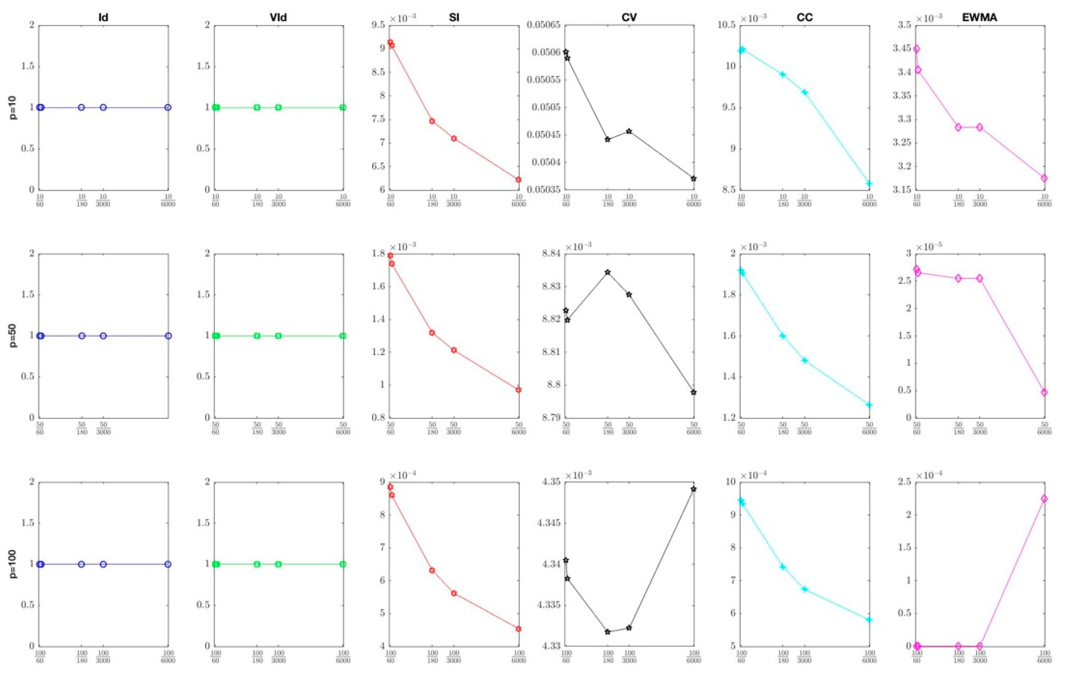
4.1.1. Results on Portfolio Weights

Table 3. Frobenius norm for the portfolio weights. Values are averaged along with the shrinkage intensity (excluding the case $\delta =0$ ). For each $n$, the first line reports the Frobenius norm for the sample covariance matrix. Abbreviations in use are: S for sample covariance; Id for identity matrix; VId for Variance Identity; SI for Single-Index; CV for Common Covariance; CC for Constant Correlation and EWMA for Exponentially Weighted Moving Average.

	P = 10				P = 50				P = 100
	MV	IV	ERC	MD	MV	IV	ERC	MD	MV	IV	ERC	MD
Panel A: n = 60
S	0.834	0.1585	0.1736	0.5842	0.7721	0.0573	0.0637	0.4933	0.7555	0.0409	0.0447	0.4565
Id	0.6863	0.1425	0.1528	0.5045	0.6215	0.0559	0.0631	0.3873	0.4967	0.0404	0.0451	0.3652
VId	0.6935	0.1583	0.1732	0.5176	0.5999	0.0567	0.0634	0.4092	0.5901	0.0404	0.0445	0.3686
SI	0.838	0.1585	0.1736	0.5678	0.7685	0.0573	0.0637	0.4709	0.75	0.0409	0.0447	0.4288
CV	1.2438	0.1583	0.1731	1.011	1.1484	0.0567	0.0628	0.9381	1.1386	0.0404	0.0438	0.9185
CC	0.8353	0.1585	0.1733	0.5361	0.7808	0.0573	0.0635	0.4328	0.7663	0.0409	0.0445	0.3922
EWMA	0.8473	0.1593	0.1745	0.595	0.7811	0.0575	0.064	0.5142	0.7325	0.0411	0.045	0.4431
Panel B: n = 120
S	0.9064	0.0877	0.0989	0.4649	0.7814	0.059	0.0656	0.5065	0.6519	0.0424	0.0472	0.4332
Id	0.8157	0.087	0.0983	0.4256	0.6259	0.0613	0.0688	0.4354	0.6307	0.0389	0.0431	0.328
VId	0.8235	0.0871	0.0985	0.4284	0.6259	0.0613	0.0688	0.4354	0.489	0.0421	0.0471	0.3712
SI	0.9097	0.0877	0.0989	0.4563	0.7777	0.059	0.0656	0.4925	0.6458	0.0424	0.0472	0.419
CV	1.3269	0.0871	0.0982	0.9667	1.1806	0.0587	0.0651	1.0138	1.0974	0.0421	0.0467	0.8951
CC	0.905	0.0877	0.0988	0.4357	0.7822	0.059	0.0655	0.4636	0.6566	0.0424	0.0471	0.3856
EWMA	0.9281	0.0883	0.0996	0.4859	0.7994	0.0592	0.0658	0.5246	0.6788	0.0427	0.0475	0.4601
Panel C: n = 180
S	0.7989	0.1311	0.1423	0.5007	0.7932	0.0564	0.0627	0.4631	0.6905	0.0404	0.044	0.4065
Id	0.7206	0.1308	0.142	0.4736	0.6705	0.0562	0.0625	0.405	0.5477	0.0375	0.0399	0.3748
VId	0.7273	0.1308	0.1421	0.4757	0.6838	0.0562	0.0626	0.4127	0.5754	0.0402	0.044	0.3556
SI	0.8001	0.1311	0.1423	0.4954	0.7904	0.0564	0.0627	0.4545	0.6873	0.0404	0.044	0.3982
CV	1.2715	0.1308	0.1419	0.9961	1.2073	0.0562	0.0624	0.9988	1.1422	0.0402	0.0437	0.8705
CC	0.7957	0.1311	0.1423	0.4803	0.792	0.0564	0.0626	0.4259	0.692	0.0404	0.044	0.3672
EWMA	0.8415	0.1322	0.1435	0.526	0.8284	0.0567	0.0631	0.5005	0.7206	0.0408	0.0445	0.4429
Panel D: n = 3000
S	0.7504	0.1476	0.1596	0.3957	0.734	0.049	0.0539	0.3988	0.513	0.0384	0.0428	0.3259
Id	0.7441	0.1477	0.1597	0.3946	0.7009	0.049	0.0539	0.3872	0.4615	0.0384	0.0428	0.3096
VId	0.7437	0.1477	0.1596	0.3945	0.7043	0.049	0.0539	0.3886	0.4673	0.0384	0.0428	0.312
SI	0.7516	0.1476	0.1596	0.3955	0.7339	0.049	0.0539	0.3984	0.5123	0.0384	0.0428	0.3252
CV	1.2864	0.1477	0.1597	0.963	1.2281	0.049	0.0538	0.9954	1.1041	0.0384	0.0428	0.6822
CC	0.7488	0.1476	0.1596	0.3949	0.7316	0.049	0.0539	0.3904	0.5096	0.0384	0.0428	0.3143
EWMA	0.8563	0.1489	0.1611	0.4452	0.8161	0.0497	0.0547	0.4652	0.6244	0.0389	0.0435	0.4076
Panel E: n = 6000
S	0.9672	0.1302	0.1409	0.4821	0.5737	0.0539	0.0589	0.3481	0.5772	0.0402	0.0437	0.3436
Id	0.9496	0.1301	0.1408	0.4813	0.6095	0.0575	0.0639	0.4076	0.5449	0.0402	0.0437	0.3342
VId	0.951	0.1301	0.1409	0.4815	0.5419	0.054	0.0589	0.3401	0.5483	0.0402	0.0437	0.3354
SI	0.9688	0.1302	0.1409	0.482	0.574	0.0539	0.0589	0.3479	0.5772	0.0402	0.0437	0.3434
CV	1.4142	0.1301	0.1408	1.0034	1.1436	0.054	0.0589	0.9706	1.1422	0.0402	0.0437	0.7031
CC	0.9656	0.1302	0.1409	0.4814	0.5709	0.0539	0.0589	0.3415	0.575	0.0402	0.0437	0.3368
EWMA	1.0432	0.1312	0.1422	0.5232	0.6946	0.0547	0.0599	0.4319	0.681	0.0407	0.0444	0.4229

and

Table 4. Frobenius norm for the portfolio weights. Values corresponds to the optimal shrinkage intensity, listed after the Frobenius norm for each portfolio. We report values for the sample covariance matrix ($\delta =0$) separately in the first row of each panel. For each $n$, the first line reports the Frobenius norm for the sample covariance matrix. Abbreviations used are: S for sample covariance; Id for identity matrix; VId for Variance Identity; SI for Single-Index; CV for Common Covariance; CC for Constant Correlation and EWMA for Exponentially Weighted Moving Average.

	P = 10				P = 50				P = 100
	MV	IV	ERC	MD	MV	IV	ERC	MD	MV	IV	ERC	MD
Panel A: n = 60
S	0.8340	0.1585	0.1736	0.5842	0.7721	0.0573	0.0637	0.4933	0.7555	0.0409	0.0447	0.4565
Id	0.6778	0.1424	0.1525	0.501	0.5997	0.0558	0.0624	0.3704	0.471	0.0403	0.0446	0.3462
VId	0.6689	0.1581	0.173	0.5084	0.5539	0.0565	0.0627	0.3795	0.5428	0.0402	0.0437	0.3331
SI	0.8345	0.1585	0.1735	0.558	0.7666	0.0573	0.0637	0.4633	0.7479	0.0409	0.0447	0.4195
CV	1.2392	0.1581	0.1729	0.509	1.117	0.0565	0.0627	0.3795	1.1068	0.0402	0.0437	0.3331
CC	0.8335	0.1585	0.1731	0.5081	0.7733	0.0573	0.0634	0.3795	0.757	0.0409	0.0444	0.3332
EWMA	0.8331	0.1586	0.1737	0.5852	0.7706	0.0573	0.0637	0.4953	0.7213	0.0409	0.0447	0.4395
Panel B: n = 120
S	0.9064	0.0877	0.0989	0.4649	0.7814	0.059	0.0656	0.5065	0.6519	0.0424	0.0472	0.4332
Id	0.8121	0.087	0.0981	0.4241	0.6119	0.0613	0.0685	0.4255	0.613	0.0388	0.0428	0.3111
VId	0.8121	0.087	0.0982	0.4242	0.6119	0.0613	0.0685	0.4255	0.4425	0.042	0.0467	0.3445
SI	0.907	0.0877	0.0989	0.4526	0.776	0.059	0.0656	0.4872	0.6431	0.0424	0.0472	0.414
CV	1.3269	0.087	0.0981	0.4245	1.1756	0.0586	0.0651	0.4302	1.0916	0.042	0.0467	0.3445
CC	0.9043	0.0877	0.0987	0.4241	0.781	0.059	0.0654	0.4302	0.6527	0.0424	0.0471	0.3446
EWMA	0.9052	0.0876	0.0988	0.4651	0.7797	0.0589	0.0655	0.5056	0.6554	0.0424	0.0472	0.4331
Panel C: n = 180
S	0.7989	0.1311	0.1423	0.5007	0.7932	0.0564	0.0627	0.4631	0.6905	0.0404	0.044	0.4065
Id	0.7177	0.1307	0.1419	0.4724	0.6613	0.0562	0.0624	0.3977	0.534	0.0375	0.0398	0.3645
VId	0.718	0.1307	0.1419	0.4724	0.6614	0.0562	0.0624	0.3979	0.5428	0.0402	0.0437	0.3331
SI	0.799	0.1311	0.1423	0.4929	0.7897	0.0564	0.0627	0.4515	0.6863	0.0404	0.044	0.3955
CV	1.2715	0.1307	0.1418	0.4724	1.2073	0.0562	0.0624	0.3979	1.1422	0.0402	0.0437	0.3331
CC	0.7942	0.1311	0.1422	0.4725	0.7912	0.0564	0.0626	0.3977	0.6904	0.0404	0.0439	0.3331
EWMA	0.8035	0.1312	0.1424	0.5008	0.7951	0.0564	0.0626	0.4653	0.6938	0.0404	0.044	0.4074
Panel D: n = 3000
S	0.7504	0.1476	0.1596	0.3957	0.734	0.049	0.0539	0.3988	0.513	0.0384	0.0428	0.3259
Id	0.7425	0.1477	0.1596	0.3941	0.6988	0.049	0.0538	0.3859	0.4573	0.0384	0.0428	0.3072
VId	0.7426	0.1476	0.1596	0.3941	0.6988	0.049	0.0538	0.3859	0.4573	0.0384	0.0428	0.3072
SI	0.7506	0.1476	0.1596	0.3953	0.7339	0.049	0.0539	0.3983	0.512	0.0384	0.0428	0.325
CV	1.2864	0.1476	0.1596	0.3951	1.2281	0.049	0.0538	0.3859	1.1041	0.0384	0.0428	0.3072
CC	0.7477	0.1476	0.1596	0.3946	0.7299	0.049	0.0539	0.386	0.5073	0.0384	0.0428	0.3072
EWMA	0.7615	0.1477	0.1597	0.3981	0.7439	0.0491	0.0539	0.4043	0.5263	0.0384	0.0429	0.3346
Panel E: n = 6000
S	0.9672	0.1302	0.1409	0.4821	0.5737	0.0539	0.0589	0.3481	0.5772	0.0402	0.0437	0.3436
Id	0.9486	0.13	0.1408	0.4811	0.6085	0.0575	0.0639	0.4072	0.5428	0.0402	0.0437	0.3331
VId	0.9486	0.13	0.1408	0.4811	0.5365	0.054	0.0589	0.3381	0.5428	0.0402	0.0437	0.3331
SI	0.9675	0.1302	0.1409	0.482	0.5738	0.0539	0.0589	0.3478	0.5772	0.0402	0.0437	0.3433
CV	1.4142	0.13	0.1408	0.4811	1.1436	0.054	0.0589	0.3381	1.1422	0.0402	0.0437	0.3331
CC	0.9644	0.1302	0.1409	0.4812	0.5687	0.0539	0.0589	0.3381	0.5733	0.0402	0.0437	0.3331
EWMA	0.9765	0.1302	0.1409	0.4832	0.5901	0.054	0.059	0.3561	0.59	0.0402	0.0438	0.3524

present the main results of the Monte Carlo study: for each combination of $p$ and $n$, we report the Monte Carlo estimator of the Frobenius norm between the true and estimated weights. In particular, Table 3 reports averaged Frobenius norm along with the shrinkage intensity (excluding the case $\delta =0$, which corresponds to the sample covariance matrix), while Table 4 lists the minimum values for the optimal shrinkage intensity.

In both tables, we compare the six target matrices by examining one risk-based portfolio at a time and the effect of increasing $p$ for fixed $n$. Special attention is devoted to the cases when $p>n$: the high-dimensional sample. We have this scenario only when $p=100$ and $n=60$. Here, the sample covariance matrix becomes ill-conditioned (Marčenko and Pastur 1967), thus it is interesting to evaluate gains obtained with shrinkage. The averaged Frobenius norm values in Table 3 give us a general overview about how target matrices perform across the whole shrinkage intensity spectrum in one goal. We aim to understand if, in average terms, shrinking the covariance matrix benefits risk-portfolio weights. On the other hand, the minimum Frobenius norm values help us understanding to what extent the various target matrices can help reproducing the true portfolio weights: the more intensity we need, the better the target is. In both tables, sample values are listed in the first row of each Panel.

Starting from Table 3, Panel A, the Minimum Variance allocation seems better described by the Identity and the Variance Identity regardless of the number of assets $p$. In particular, we look at the difference between the weights calculated entirely on the sample covariance matrix and those of the targets: the Identity and the Variance Identity are the only estimator to perform better. In fact, shrinking towards the sample is not as bad as shrinking towards the Common Covariance. By increasing $n$ and moving to Panel B, similar results are obtained. This trend is confirmed in Panel C, while in the cases of $n=3000$ and $n=6000$, all the estimators perform similarly. Hence, for the Minimum Variance portfolio the Identity matrix works best at reproducing portfolio weights very similar to the true ones. The same conclusions apply for the Maximum Diversification portfolio: when $p$ and $n$ are small, the Identity and the Variance Identity outperform other alternatives. On the other hand, we get very different results for the Inverse Volatility and Equal-Risk-Contribution. Both portfolios seem not gaining benefits from the shrinkage procedure, as the Frobenius norm is very similar to that of the sample covariance matrix for all the target matrices under consideration. This is true for all pairs of $p$ and $n$. In the high-dimensional case ($p=100$; $n=60$), the Identity matrix works best in reducing the distance between true and estimated portfolio weights, both for the Minimum Variance and Maximum Diversification portfolios. On average, shrinkage does not help too much when alternative target matrices are used; only in the case of Common Covariance is shrinking worse than using the sample covariance matrix. All these effects vanish when we look at the Inverse Volatility and Equal-Risk-Contribution portfolios: here, shrinkage does not help too much, whatever the target is.

Overall, results are in line with the conclusions of the numerical illustrations in Section 3. Indeed, the Minimum Variance portfolio shows the highest distance between true and estimated weights, similar to the Maximum Diversification. Both portfolios are affected by the dimensionality of the sample: shrinkage always help in reducing weights misspecification; it improves in high-dimensional cases. On contrary, estimated weights for the remaining portfolios are close to the true ones by construction, hence, shrinkage does not help too much.

Switching to Table 4, the results illustrate again that the Identity and the Variance Identity attain the best reduction of the Frobenius norm for the Minimum Variance and Maximum Diversification portfolios. If results are similar to those of Table 3 for the former, results for the latter show an improvement in using the shrinkage estimators. The Identity, Variance Identity, Common Covariance, and Constant Correlation target matrices outperform all the alternatives, including the sample estimator, minimising the Frobenius norm in a similar fashion. This is true also for the high-dimensional case. On the contrary, the other two portfolios do not benefit from shrinking the sample covariance matrix, even in high-dimensional samples, confirming the insights from Table 3. Lastly, we look at the shrinkage intensity at which target matrices attain the highest Frobenius norm reduction. Those values are displayed in Figure 4. The intensity is composed of the interval $\left[0;1\right]$: the more it is close to 1, the more the target matrix helps in reducing the estimation error of the sample covariance matrix. Interestingly, the Identity and the Variance Identity show shrinkage intensities always close to 1, meaning that shrinking towards them is highly beneficial, as they are fairly better than the sample covariance matrix. This is verified either for the high-dimensional case and for those risk portfolios (Inverse Volatility and Equal-Risk-Contribution), who do not show great improvements when shrinkage is adopted.

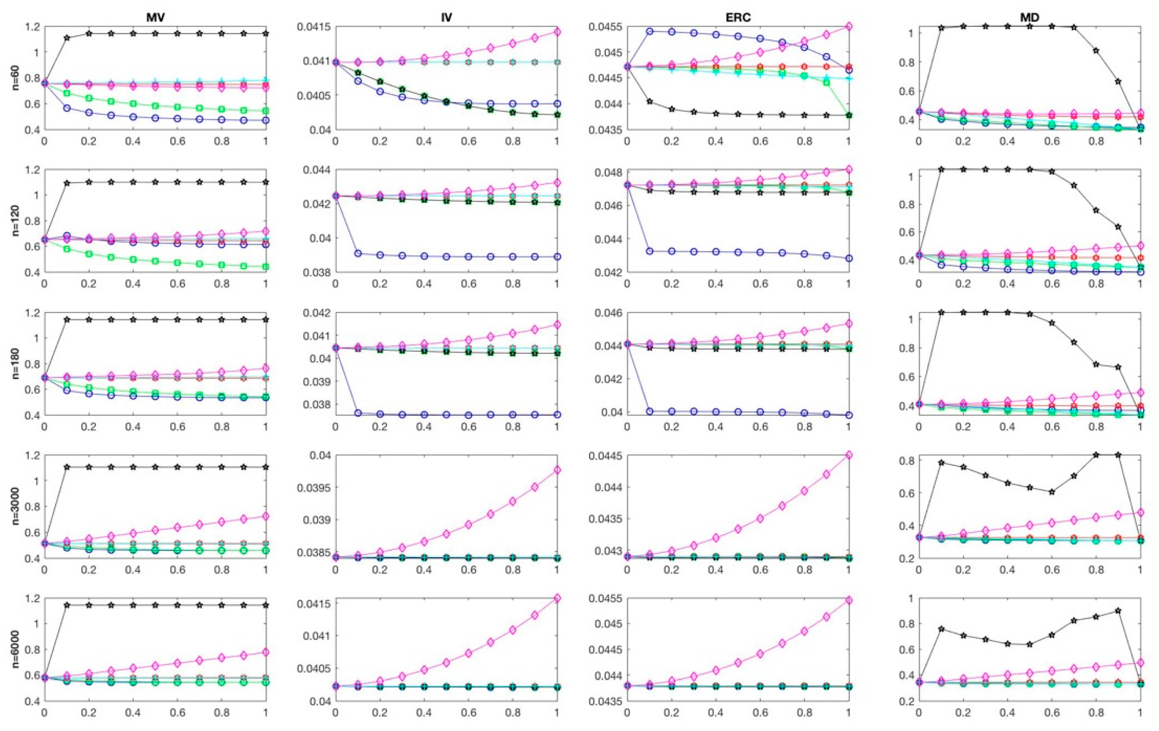
4.1.2. Sensitivity to Shrinkage Intensity

To have a view on the whole shrinkage intensity spectrum (i.e., the interval $\left(0;1\right)$) we refer to Figure 5, where we report the Frobenius Norms for the weights (y-axis) with regard to the shrinkage intensity (x-axis). Each column corresponds to a specific risk-based portfolio: from left to right, the Minimum Variance, the Inverse Volatility, the Equal-Risk-Contribution, and the Maximum Diversification, respectively. Each row corresponds to the $p/n$ ratio in $n$ ascending order. For each subfigure, the Identity is blue circle-shaped, the Variance Identity is green square-shaped, the Single-Index is red hexagram-shaped, the Common Covariance is black star-shaped, the Constant Correlation is cyan plus-shaped, and the EWMA is magenta diamond-shaped.

Figure 5 illustrates the case $p=100$, as to include the high-dimensional scenario. Starting from the latter (first row, $n=60$), the Variance Identity is the only target matrix to always reduce weight misspecification for all the considered portfolios, for all shrinkage levels. The Identity do the same, excluding the ERC case where it performs worse than the sample covariance matrix. The remaining targets behave very differently across the four risk-based portfolios: the Common Covariance is the worst in both the Minimum Variance and Maximum Diversification and the EWMA is the worst in both remaining portfolios. The Market Model and the Constant Correlation do not improve much from the sample estimator across all portfolios.

Looking at the second row ($n=120$), the Identity is the most efficient target, reducing the distance between estimated and true portfolio weights in all the considered portfolios. The Variance Identity is also very efficient in Minimum Variance and Maximum Diversification portfolios, while the remaining targets show similar results as in the previous case. The same conclusions apply for the case $n=180$.

When the number of observations is equal to or higher than $n=3000$, results do not change much. The Identity, the Variance Identity, the Market model, and the Constant Correlation are the most efficient target matrices towards which to shrink, while the EWMA is the worst for both Inverse Volatility and Equal-Risk-Contribution portfolios and the Common Covariance is the worst for the Minimum Variance and Maximum Diversification ones.

In conclusion, for the Minimum Variance portfolio, the Common Covariance should not be used, since it always produces weights very unstable and distant from the true ones. At the same time, the EWMA should not be used to shrink the covariance matrix in the Inverse Volatility and Equal-Risk-Contribution portfolios. The most convenient matrices towards which to shrink are the Identity and the Variance Identity. Overall, the Minimum Variance and the Maximum Diversification portfolio weights gain more from shrinkage than those of the Inverse Volatility and Equal-Risk-Contribution allocations.

5. Conclusions

In this article, we provide a comprehensive overview of shrinkage in risk-based portfolios. Portfolios solely based on the asset returns covariance matrix are usually perceived as “robust” since they avoid estimating the asset returns mean. However, they still suffer from estimation error when the sample estimator is used, causing misspecification in the portfolio weights. Shrinkage estimators have been proved to reduce the estimation error by pulling the sample covariance towards a more structured target.

By means of an extensive Monte Carlo study, we compare six different target matrices: the Identity, the Variance Identity, the Single-index model, the Common Covariance, the Constant Correlation, and the Exponential Weighted Moving Average, respectively. We do so considering their effects on weights for the Minimum Variance, Inverse Volatility, Equal-risk-contribution, and Maximum diversification portfolios. Moreover, we control for the whole shrinkage intensity spectrum and for dataset size, changing observation length and number of assets. Therefore, we are able to (1) assess estimators’ statistical properties and similarity with the true target matrix; (2) address the problem of how selecting a specific target estimator affects the portfolio weights.

Regarding point (1), the findings suggest the Identity and the Variance Identity matrices hold the best statistical properties, being well conditioned across all the combinations of observations/assets, especially for high-dimensional datasets. Nevertheless, these targets are both not very similar to the true target matrix. The Single-Index and the Constant Correlation target matrices show the greater similarity with the true target matrix, minimizing the Frobenius norm, albeit being poorly conditioned when observations and assets share similar sizes. Turning to point (2), the Identity attains the best results in terms of distance reduction between the true and estimated portfolio weights for both the Minimum Variance and Maximum Diversification portfolio construction techniques. The Variance Identity shows a similar performance. Both estimators are also stable against shifts in the shrinkage intensity.

Overall, selecting the target matrix is very important, since we verified that there are large shifts in the distance between true and estimated portfolio weights when shrinking towards different targets. In risk-based portfolio allocations the Identity and the Variance Identity matrices represent the best target among the six considered in this study, especially in the case of Minimum Variance and Maximum Diversification portfolios. In fact, they are always well conditioned and outperform their competitor in deriving the most similar weights to the true ones.

Lastly, the findings confirm that the Minimum Variance and Maximum Diversification portfolios are more sensitive to misspecification in the covariance matrix, therefore, they benefit the most when the sample covariance matrix is shrunk. These findings are in line with what was previously found in Ardia et al. (2017): the Inverse Volatility and the Equal-Risk-Contribution are more robust to covariance misspecification; hence, allocations do not improve significantly when shrinkage is used.

References

1. Ardia, David, Guido Bolliger, Kris Boudt, and Jean Philippe Gagnon-Fleury. 2017. The Impact of Covariance Misspecification in Risk-Based Portfolios. Annals of Operations Research 254: 1–16. [Google Scholar] [CrossRef]
2. Black, Fischer, and Robert Litterman. 1992. Global Portfolio Optimization. Financial Analysts Journal 48: 28–43. [Google Scholar] [CrossRef] [Green Version]
3. Briner, Beat G., and Gregory Connor. 2008. How Much Structure Is Best? A Comparison of Market Model, Factor Model and Unstructured Equity Covariance Matrices. Journal of Risk 10: 3–30. [Google Scholar] [CrossRef]
4. Candelon, Bertrand, Christophe Hurlin, and Sessi Tokpavi. 2012. Sampling Error and Double Shrinkage Estimation of Minimum Variance Portfolios. Journal of Empirical Finance 19: 511–27. [Google Scholar] [CrossRef]
5. Chopra, Vijay Kumar, and William T. Ziemba. 1993. The Effect of Errors in Means, Variances, and Covariances on Optimal Portfolio Choice. The Journal of Portfolio Management 19: 6–11. [Google Scholar] [CrossRef]
6. Choueifaty, Yves, and Yves Coignard. 2008. Toward Maximum Diversification. The Journal of Portfolio Management 35: 40–51. [Google Scholar] [CrossRef]
7. De Miguel, Victor, Lorenzo Garlappi, and Raman Uppal. 2009. Optimal versus Naive Diversification: How Inefficient Is the 1/N Portfolio Strategy? Review of Financial Studies 22: 1915–53. [Google Scholar] [CrossRef]
8. De Miguel, Victor, Alberto Martin-Utrera, and Francisco J. Nogales. 2013. Size Matters: Optimal Calibration of Shrinkage Estimators for Portfolio Selection. Journal of Banking and Finance 37: 3018–34. [Google Scholar] [CrossRef]
9. J., P. Morgan, and Reuters Ltd. 1996. Risk Metrics—Technical Document, 4th ed. New York: Morgan Guaranty Trust. [Google Scholar]
10. Jagannathan, Ravi, and Tongshu Ma. 2003. Risk Reduction in Large Portfolios: Why Imposing the Wrong Constraints Helps. Journal of Finance 58: 1651–84. [Google Scholar] [CrossRef]
11. James, W., and Charles Stein. 1961. Estimation with Quadratic Loss. In Proceedings of the 4th Berkeley Symposium on Probability and Statistics, Volume 1. Paper presented at Fourth Berkeley Symposium on Mathematical Statistics and Probability, Berkeley, CA, USA, June 20–July 30. [Google Scholar]
12. Jorion, Philippe. 1986. Bayes-Stein Estimation for Portfolio Analysis. The Journal of Financial and Quantitative Analysis 21: 279–92. [Google Scholar] [CrossRef]
13. Ledoit, Olivier, and Michael Wolf. 2003. Improved Estimation of the Covariance Matrix of Stock Returns with an Application to Portfolio Selection. Journal of Empirical Finance 10: 603–21. [Google Scholar] [CrossRef]
14. Ledoit, Olivier, and Michael Wolf. 2004a. A Well-Conditioned Estimator for Large-Dimensional Covariance Matrices. Journal of Multivariate Analysis 88: 365–411. [Google Scholar] [CrossRef]
15. Ledoit, Olivier, and Michael Wolf. 2004b. Honey, I Shrunk the Sample Covariance Matrix—Problems in Mean-Variance Optimization. Journal of Portfolio Management 30: 110–19. [Google Scholar] [CrossRef]
16. Leote de Carvalho, Raul, Xiao Lu, and Pierre Moulin. 2012. Demystifying Equity Risk–Based Strategies: A Simple Alpha plus Beta Description. The Journal of Portfolio Management 38: 56–70. [Google Scholar] [CrossRef]
17. MacKinlay, A. Craig, and Lubos Pastor. 2000. Asset Pricing Models: Implications for Expected Returns and Portfolio Selection. Review of Financial Studies 13: 883–916. [Google Scholar] [CrossRef]
18. Maillard, Sébastien, Thierry Roncalli, and Jérôme Teïletche. 2010. The Properties of Equally Weighted Risk Contribution Portfolios. The Journal of Portfolio Management 36: 60–70. [Google Scholar] [CrossRef]
19. Marčenko, Vladimir Alexandrovich, and Leonid Andreevich Pastur. 1967. Distribution of Eigenvalues for Some Sets of Random Matrices. Mathematics of the USSR-Sbornik 1: 507–36. [Google Scholar] [CrossRef]
20. Markowitz, Harry. 1952. Portfolio Selection. The Journal of Finance 7: 77–91. [Google Scholar] [CrossRef]
21. Markowitz, Harry. 1956. The Optimization of a Quadratic Function Subject to Linear Constraints. Naval Research Logistics Quarterly 3: 111–33. [Google Scholar] [CrossRef]
22. Merton, Robert C. 1980. On Estimating the Expected Return on the Market: An Exploratory Investigation. Topics in Catalysis 8: 323–61. [Google Scholar]
23. Michaud, Richard O. 1989. The Markowitz Optimization Enigma: Is Optimized Optimal? Financial Analysts Journal 45: 31–42. [Google Scholar] [CrossRef]
24. Pantaleo, Ester, Michele Tumminello, Fabrizio Lillo, and Rosario N. Mantegna. 2011. When Do Improved Covariance Matrix Estimators Enhance Portfolio Optimization? An Empirical Comparative Study of Nine Estimators. Quantitative Finance 11: 1067–80. [Google Scholar] [CrossRef]
25. Qian, Edward. 2006. On the Financial Interpretation of Risk Contribution: Risk Budgets Do Add Up. Journal of Investment Management 4: 41–51. [Google Scholar] [CrossRef]
26. Schäfer, Juliane, and Korbinian Strimmer. 2005. A Shrinkage approach to large-scale covariance matrix estimation and implications for functional genomics. Applications in Genetics and Molecular Biology 4: 1175–89. [Google Scholar] [CrossRef] [PubMed]
27. Sharpe, William F. 1963. A simplified model for portfolio analysis. Management Science 9: 277–93. [Google Scholar] [CrossRef]
1
The majority of papers on risk-based portfolios are published in journal aimed at practitioners, as the Journal of Portfolio Management.
2
With this we refer to the population covariance matrix, which by definition is not observable and then unfeasible. Hence, Σ is estimated taking into account the observations stored in X: we will deeply treat this in the next section.
3
The sample covariance matrix is the Maximum Likelihood Estimator (MLE) under Normality, therefore it lets data speaks without imposing any structure.
4
In reality, we exclude the Scaled Identity of De Miguel et al. (2013) because of its great similarity with the Identity and Variance Identity implemented in our study.
5
Ardia et al. (2017) imposes Asset-1 and Asset-2 to have 10% annual volatility; Asset-3 to have 20% annual volatility; correlations between Asset-1/Asset-2 and Asset-1/Asset-3 are set as negative and correlation between corporate bonds and equities (Asset-2/Asset-3) is set as positive. However, to better resemble real data, specifically the S&P500, the US corporate index and the US Treasury Index total returns, we assume all three correlation parameters to be positive.
6
7
Simulations were done in MATLAB setting the random seed generator at its default value, thus ensuring the full reproducibility of the analysis. Related code available at the GitHub page of the author: https://github.com/marconeffelli/Risk-Based-Portfolios.
Figure 1. Frobenius norm between true and estimated weights; first row reports misspecification in volatility, while second row in correlation. The surfaces’ three dimensions are: the shrinkage intensity in y axis (from 0 to 1); the misspecification in the volatility (from 0 to 0.5) or in the correlation (from 0 to 1) in x axis and the Frobenius norm in z axis. Each column refers to a specific risk-based portfolio. From the left to the right: Minimum Variance (MV), Inverse Volatility (IV), Equal-Risk-Contribution (ERC), Maximum Diversification (MD), respectively.
Risks 06 00125 g001
Figure 2. The reciprocal 1-norm condition number (y-axis) as the p / n ratio moves from p 60 to p 6000 (x-axis). Each column corresponds to a specific target matrix: from left to right, the Identity (Id): blue circle-shaped; the Variance Identity (VId): green square-shaped; the Single-Index (SI): red hexagram-shaped; the Common Covariance (CV): black star-shaped; the Constant Correlation (CC): cyan plus-shaped; and the Exponential Weighted Moving Average (EWMA): magenta diamond-shaped, respectively. Each row corresponds to a different p : in ascendant order from 10 (first row) to 100 (third row).
Risks 06 00125 g002
Figure 3. Surfaces representing the Frobenius norm (z-axis) between the true and the estimated target matrices, considering the shrinkage intensity (y-axis) and the p / n ratio (x-axis). Each column corresponds to a specific target matrix: from left to right, the Identity (Id), the Variance Identity (VId), the Single-Index (SI), the Common Covariance (CV), the Constant Correlation (CC), and the EWMA, respectively. Each row corresponds to a different p : in ascendant order from p = 10 (first row) to p = 100 (third row).
Risks 06 00125 g003
Figure 4. Optimal shrinkage intensity parameters for which the Frobenius norm is minimized. Each column corresponds to a specific target matrix: from left to right, the Identity, the Variance Identity, the Single-Index, the Common Covariance, the Constant Correlation, and the EWMA, respectively. Each row corresponds to a different n : in ascendant order from n = 60 (first row) to p = 6000 (fifth row). In each subplot, the MV portfolio is blue circle-shaped; the IV is green-square shaped; the ERC is red-triangle shaped; and the MD is black-cross shaped.
Risks 06 00125 g004
Figure 5. Frobenius norm for portfolio weights with regard to the shrinkage intensity parameter, when p = 100 .
Risks 06 00125 g005