Mortality Forecasting: How Far Back Should We Look in Time?

Abstract

Extrapolative methods are one of the most commonly-adopted forecasting approaches in the literature on projecting future mortality rates. It can be argued that there are two types of mortality models using this approach. The first extracts patterns in age, time and cohort dimensions either in a deterministic fashion or a stochastic fashion. The second uses non-parametric smoothing techniques to model mortality and thus has no explicit constraints placed on the model. We argue that from a forecasting point of view, the main difference between the two types of models is whether they treat recent and historical information equally in the projection process. In this paper, we compare the forecasting performance of the two types of models using Great Britain male mortality data from 1950–2016. We also conduct a robustness test to see how sensitive the forecasts are to the changes in the length of historical data used to calibrate the models. The main conclusion from the study is that more recent information should be given more weight in the forecasting process as it has greater predictive power over historical information.

1. Introduction

Accurate future mortality forecasts are of fundamental importance as they ensure adequate pricing of mortality-linked insurance and financial products. Hence, there is an increasing need to have a better understanding of mortality in order to increase the accuracy of mortality forecasts.

In the literature of mortality modelling, many attempts have been made to project future mortality rates using different types of models1. Most of these models tend to identify patterns in age, time or cohort dimensions in the mortality data and extract these patterns to make projections on future mortality rates. There have been a number of studies on the comparison of the forecasting performances of different models (Cairns et al. 2011; Haberman and Renshaw 2009; Hyndman and Ullah 2007), and the quantitative and qualitative criteria used include: the overall accuracy; allowance for cohort effect; biological reasonableness; and the robustness of forecast. However, as far as we know, very few studies have considered the question of whether a mortality model should treat past and recent mortality experience equally in the forecasting process (see the discussions in Li et al. (2015, 2016)).

We argue that mortality forecasting models can be divided into two categories: one uses local information (i.e., gives higher weight to recent mortality data), and the other uses global information (i.e., gives equal weight to past and recent mortality data). Examples of models falling in the first category include the P-splines model by Currie et al. (2004), the two-dimensional thin plate model by Dokumentov and Hyndman (2014) and the two-dimensional kernel smoothing (2D KS) model by Li et al. (2016). Examples of models using global information to produce mortality forecast include the well-known Lee–Carter model (Lee and Carter 1992), the Cairns–Blake–Dowd (CBD) model (Cairns et al. 2006), the Plat model (Plat 2009) and the two-dimensional Legendre orthogonal polynomial (2D LOP) model proposed by Li et al. (2017).

Therefore, one of the primary interests of this paper is to look at the question of whether local or global information is more appropriate to use and thus should be preferred in the mortality forecasting process. We include two pairs of mortality models for comparison. In order to control the number of factors that will influence the forecasting performance of mortality models, in each group, apart from this difference in the forecasting approach, the design and structure of the two models bear great similarity. A detailed study is conducted using male mortality data of Great Britain from 1950–2016 for ages 50–89. Based on the empirical results from a multi-year-ahead backtesting exercise, we compare and comment on the differences in the forecasting performances across the two groups of models and conclude that local information is more relevant to produce accurate mortality forecast. Further, the robustness test shows that all four models included in the analysis appear to be reasonably robust relative to the changes in the length of historical data employed in the estimation.

The plan of the paper is as follows. Section 2 reviews and provides details of the models to be compared in this study. In Section 3, we conduct a case study and comment on the forecasting performances of the models described in Section 2. Finally, Section 4 draws the conclusions and also gives future research directions.

2. Models for Comparison

This section begins by defining some actuarial notation in the mortality modelling literature, which we are going to use throughout the paper. We then conduct a brief review of the models being compared in this study. These include the CBD model (Cairns et al. 2006) and its local linear approach proposed by Li et al. (2015), the 2D LOP model (Li et al. 2017) and the 2D KS model (Li et al. 2016). We divide these models into two groups based on the similarity in their model designs and inclusion or not of cohort effects.

2.1. Notation

Recent mortality studies generally model two types of mortality rates: central mortality rates (see for example Lee and Carter (1992); Hyndman and Ullah (2007)) and initial mortality rates (see for example Cairns et al. (2006); Li and O’Hare (2017)). For $x\in [a+1,a+N]$ and $t\in [1,T]$, where a, T and N are non-negative integers, define:

• $d_{x,t}$ as the observed number of deaths in calender year t aged x.
• $e_{x,t}$ as the exposure data that measure the average population in calendar year t aged x.
• $m_{x,t}$ as the central mortality rate, which reflects the death probability at age x in the middle of the year. It is calculated by:

  $$m_{x,t}=\frac{d_{x,t}}{e_{x,t}}.$$

  (1)
• $q_{x,t}$ as the initial mortality rate, which is the one-year death probability for a person who is aged exactly x at time t.

Numerically, the central mortality rate and initial mortality rate are quite close in their values. The approximation formula for the two types of mortality rates is as follows2:

$$q_{x,t}=1-\exp (-m_{x,t}).$$

(2)

2.2. CBD Model and a Local Linear Approach

In the new era of stochastic mortality modelling, the CBD model is considered as a strong contender among different stochastic models. It was introduced by Cairns et al. (2006), and the model utilizes the exponential dynamics in older age mortality described by the Gompertz law Gompertz (1825). The CBD model is of the form:

$$\mathrm{logit}\left(q_{x,t}\right)=\log \left(\frac{q_{x,t}}{1-q_{x,t}}\right)={\kappa }_t^1+{\kappa }_t^2(x-\overline{x})+{ϵ}_{x,t},$$

(3)

where ${\kappa }_t^1$ and ${\kappa }_t^2$ are time-related effects and $\overline{x}$ is the average age in the sample range.

The parameters in the CBD model can be estimated using the maximum likelihood estimation (MLE) approach proposed by Brouhns et al. (2002) based on a Poisson error structure. It provides good fitting and forecasting results for a number of countries’ mortality experience, and since there are multiple factors in the model, it has a non-trivial correlation structure Cairns et al. (2006). For the purpose of future mortality projection, (${\kappa }_t^1$, ${\kappa }_t^2$) is normally treated as a bivariate random walk with drift process. Define ${\beta }_t=\left(\begin{array}{c}{\kappa }_t^1\\ {\kappa }_t^2\end{array}\right)$; we have:

$${\beta }_t={\beta }_{t-1}+\mu +C{Z}_t,$$

(4)

where $\mu$ is a column vector of the drift factors and $Z_t$ is a column vector of independent standard normal random variables. C is an upper triangular matrix by Cholesky decomposition of the variance-covariance matrix of ${\kappa }_t^1$ and ${\kappa }_t^2$. The drift factors and variance-covariance matrix can be estimated from the MLE estimators ${\widehat{\kappa }}_t^1$ and ${\widehat{\kappa }}_t^2$.

Thus, the one-year-ahead forecast of ${\beta }_t$ is given by:

$${\beta }_{T+1}={\beta }_T+\widehat{\mu }+\widehat{C}{Z}_{T+1}.$$

(5)

The work in Li et al. (2015) explored the possibility of ${\kappa }_t^1$ and ${\kappa }_t^2$ being smooth functions of time and introduced a local linear estimation (LLE) and forecasting approach to the model. The CBD model was re-expressed as a semi-parametric time-varying coefficient model, as we define, for $x\in [a+1,a+N]$ and $t\in [1,T]$,

• $Y_{it}=\mathrm{logit}\left(q_{x,t}\right)$ and ${ϵ}_{it}={ϵ}_{x,t}$, where $i=x-a$ denotes age groups.
• $X_i=$$\left(\begin{array}{c}1\\ x-\overline{x}\end{array}\right).$
• ${\beta }_t=$$\left(\begin{array}{c}{\kappa }_t^1\\ {\kappa }_t^2\end{array}\right)$ where ${\kappa }_t^1$ and ${\kappa }_t^2$ are smooth functions of t.

Thus, the model becomes:

$$Y_{it}=\mathrm{logit}\left(q_{x,t}\right)={\kappa }_t^1+{\kappa }_t^2(x-\overline{x})+{ϵ}_{x,t}=X_i^{\prime }{\beta }_t+{ϵ}_{it}.$$

(6)

Li et al.’s approach treats ${\beta }_t$ as a smooth function of time and defines ${\beta }_t=\beta \left(\tau \right),\mathrm{where}\tau =t/T$ and $t\in [1,T]$. Thus, by Taylor expansion, for any given ${\tau }_0\in [0,1]$, the model can be approximated by:

$$Y_{it}=X_i^{\prime }\beta \left(\tau \right)\approx X_i^{\prime }[\beta \left({\tau }_0\right)+{\beta }^{\left(1\right)}\left({\tau }_0\right)(\tau -{\tau }_0)],$$

(7)

where ${\beta }^{\left(1\right)}\left({\tau }_0\right)$ is the first order derivative at ${\tau }_0$.

The local linear estimator of $\beta \left({\tau }_0\right)$ can be obtained by minimizing the following weighted sum of squares with respect to $(\beta \left({\tau }_0\right),{\beta }^{\left(1\right)}\left({\tau }_0\right))$3:

$$\sum _{i=1}^N\sum _{t=1}^T{\{Y_{it}-X_i^{\prime }[\beta \left({\tau }_0\right)+{\beta }^{\left(1\right)}\left({\tau }_0\right)(\tau -{\tau }_0)]\}}^2{K}_h(\tau -{\tau }_0),$$

(8)

where K is the kernel function that determines the shape of kernel weights and $K_h\left(u\right)=h^{-1}K(u/h)$. h is the bandwidth, which determines the size of the weights. Following Li et al.’s work, in this paper, we use leave-one-out cross-validation as the bandwidth selection algorithm and adopt the Epanechnikov kernel function described as follows:

$$K\left(u\right)=0.75(1-u^2)I\left(\right|u|\le 1).$$

(9)

One of the strengths of this approach relies on the fact that the projection of future mortality rates can be done simultaneously with the estimation process.

2.3. 2D LOP Model and 2D KS Model

Including the CBD model, most of the recent mortality models make certain assumptions on the age, time or cohort structure of the mortality surface. Li et al. (2017) proposed a flexible functional form approach to mortality modelling through the introduction of the 2D LOP model. The model is defined as follows:

$$\log \left(m_{x,t}\right)=\sum _{m=0}^6\sum _{n=0}^6{\beta }_{m,n}{\phi }_{m,n}(x,t)+{ϵ}_{x,t},$$

(10)

where ${\phi }_{m,n}$ is the two-dimensional Legendre polynomial as described in Mádi-Nagy (2012) and ${\beta }_{m,n}$ is the coefficient for the ${(m,n)}^{\mathrm{th}}$ polynomial. The maximum order of polynomials used in this paper is six, which is consistent with Li et al.’s study (2017). As the interval of orthogonality for Legendre polynomials is $[-1,1]$, in this model, we need to normalize the x and t indexes into the range of $[-1,1]$ first. Least absolute shrinkage and selection operator (Lasso) is used as the regularization tool in the model selection procedure. For the selection of tuning parameter in Lasso estimation, we follow the study of Li et al. (2017) and use the 10-fold cross-validation method.

The one-year-ahead mortality forecast can then be obtained as:

$$\log \left(m_{x,T+1}\right)=\sum _{m=0}^6\sum _{n=0}^6{\widehat{\beta }}_{m,n}{\phi }_{m,n}(x,T+1),$$

(11)

where ${\widehat{\beta }}_{m,n}$ is the Lasso estimator of ${\beta }_{m,n}$.

Unlike some existing stochastic mortality models, the 2D LOP model does not impose any restrictions on the functional form of the model and thus allows us to tailor our model design according to different countries’ specific mortality experience. For countries with with systematic high or low mortality in some cohort groups, additional cohort dummies will be included in the model. This is to ensure the “cleanness” of the residual plot so that no important information is left unexplained in the model.

According to Härdle (1990), any modelling process involving the use of prespecified parametric functions is subject to the problem of “misspecification”, which may result in high model bias. Nonparametric techniques, on the other hand, are more flexible and data-driven, and thus, could provide a more general approach to mortality modelling Currie et al. (2004). The work in Li et al. (2016) proposed a mortality model that implements two-dimensional kernel smoothing techniques to mortality surfaces. The 2D KS model is of the form:

$$\log \left(m_{x,t}\right)=\beta (x,t)+{ϵ}_{x,t},$$

(12)

where $\beta (x,t)$ is any unknown functions of x and t. Without loss of generality, we normalize the x and t indexes into interval $[0,1]$ (Härdle, 1990). The kernel smoother at any given $x_0\in [0,1]$ and $t_0\in [0,1]$ can be obtained by solving the minimization problem as follows,

$$\widehat{\beta }(x_0,t_0)=\underset{\beta (x_0,t_0)}{argmin}\sum _x\sum _t{[\log \left(m_{x,t}\right)-\beta (x_0,t_0)]}^2{K}_{h_1,h_2}(x-x_0,t-t_0),$$

(13)

where kernel function K determines the shape of kernel weights and $K_{h_1,h_2}(x-x_0,t-t_0)=K(\frac{x-x_0}{h_1},\frac{t-t_0}{h_2})$; while the size of the weights is set by $h_1$ and $h_2$, which are bandwidths in age and time dimension respectively. Again, following Li et al. (2016), we adopt the bivariate normal kernel function with correlation $\rho \in (0,1]$ in order to capture the dependence in age and time dimensions, in other words, the cohort effect. The bandwidths and correlation parameter $\rho$ will be selected based on the out-of-sample mean squared forecast error.4

It has been shown that the model produces satisfactory fitting and forecasting results, and it also incorporates cohort effects into both the estimation and forecasting processes. To obtain one-year-ahead mortality forecast, since the time index extends to $T+1$, we first adjust t back into $[0,1]$ and set $t_0=1$. Then, the kernel estimator at $T+1$ can be computed by solving the minimization problem in Equation (13).

2.4. A Discussion on the Two Groups of Mortality Models

A common feature in this two groups of models is that, in each group, the two models are of similar designs in structures, but one mainly uses local information in the forecasting procedure and the other global information. In the first group, apart from different estimation and forecasting methodologies, the age and time structures of the two models are exactly the same. The random walk (RW) forecast uses global information to produce the mortality forecast since when estimating the drift factor $\mu$, past and recent mortality experiences are equally treated. On the other hand, based on the weight function described in Section 2.2, the local linear (LL) forecasting method will set greater weights on most recent mortality data and lighter weights on historical mortality data. Similarly, in the second group, the two models show clear similarities in the model design, as they both assume smoothness in the age and time dimensions. The difference is: the parameters in the 2D LOP model are estimated based on the entire mortality surface, and thus, the model produces the mortality forecast using global information; while the 2D KS model mainly uses local information to project future mortality rates since the kernel function assigns greater weights on recent mortality experience in the forecasting process.

The main differences between the two groups of models are: firstly, both the 2D LOP model and the 2D KS model are data-driven without prior assumptions on age, time or cohort structure of the underlying data; however, the CBD model in the first group imposes restrictions on structures in the age and time dimensions. Secondly, the CBD model does not allow for cohort effects in its model design, while both models in the second group tend to capture the cohort effect using either a parametric or nonparametric approach.

Finally, it is worth noting that the 2D KS model is the only model that is free of the “misspecification” problem mentioned earlier in this section, as it does not involve any parametric functions in the modelling process and uses a pure nonparametric approach; while both the CBD model and the 2D LOP model are subject to the problem of “misspecification” since both of them contain parametric components.

3. Case Study: GB Male Mortality Data from 1950–2016, Ages 50–89

This section starts with a description of the mortality data used in the case study. Then, we will assess the fit quality of the four models based on both statistical measures and the randomness in residual plots. To comment on the short-, medium- and long-term forecasting performances of the models, properly constituted backtesting has been carried out, and the forecasting results for various forecast horizons are presented and compared. The robustness of mortality forecasts relative to the period of data employed was also tested for each of the four models. We chose different investigation periods to see how sensitive the forecasting performance of each model was to the length of historical data used to fit the model.

3.1. Data

The dataset used in this study is: male mortality data of Great Britain (GB) during 1950–2016 for age range 50–89.5 Even though longer historical data are also available, we chose to use mortality data in this post-war time period because we believe that the data are of good quality and are more reliable. Since our primary interest was to improve the forecast accuracy for older ages, to which longevity risk is more exposed, in this study, we used the age range from 50–89. We have chosen this age range not only because the CBD model performs best among older age groups, but also because older age groups are more exposed to longevity risk, which is one of the emerging risks faced by society. This age range is also consistent and in line with other studies in the literature (see for example Cairns et al. (2009, 2011); Dowd et al. (2010)). The deaths and exposures data used to calculate central mortality rates and initial mortality rates were downloaded from the Human Mortality Database (2019).

3.2. Fit Quality and Residual Plots

Following the investigations of O’Hare and Li (2012) and Li et al. (2015), we define the following statistical measures:

• The average error ($E1$), which is a measure of overall bias, is calculated as:

  $$E1=\frac{1}{NT}\sum _x\sum _t\frac{{\widehat{m}}_{x,t}-m_{x,t}}{m_{x,t}}.$$

  (14)
• The absolute average error ($E2$), which measures the absolute size of the deviance, is calculated as:

  $$E2=\frac{1}{NT}\sum _x\sum _t\frac{|{\widehat{m}}_{x,t}-m_{x,t}|}{m_{x,t}}.$$

  (15)
• The standard deviation of error ($E3$), which is an indicator of large deviance, is calculated as:

  $$E3=\sqrt{\frac{1}{NT}{\sum }_x{\sum }_t{\left(\frac{{\widehat{m}}_{x,t}-m_{x,t}}{m_{x,t}}\right)}^2}.$$

  (16)

Table 1. Fitting results for GB male mortality data from 1950–2016, ages 50–89. CBD, Cairns–Blake–Dowd; LOP, Legendre orthogonal polynomial; KS, kernel smoothing.

	CBD Model: MLE	CBD Model: LLE	2D LOP Model	2D KS Model
$E1(\%)$	0.64	$-0.07$	0.07	0.03
$E2(\%)$	4.23	4.42	2.94	1.75
$E3(\%)$	5.73	5.52	3.63	2.34

illustrates the fitting results of the four models using the mortality data described in Section 3.1. It can be concluded that the 2D KS model gave the best fitting results among the four models on all three measures for GB male mortality data for the period 1950–2016 and ages 50–89. The 2D LOP provided a slightly worse quality of fit, but the results were still comparable with the 2D KS model. Overall, the fitting results from the second group were better than those from the CBD model for both the MLE method and the LLE method. This result is not surprising as the structure of the CBD model is relatively simple and it does not incorporate cohort effects.

Whilst all the models provided a reasonably good fit, it is worth noting, as in a recent study on mortality model comparisons by Cairns et al. (2011), that a good fit to historical data does not guarantee good forecasting performances. The work in Li et al. (2016) argued that the “cleanness” of residual plots should also be taken into account when assessing the fitting performance of the model. A check of the residual plots for the four models included in this analysis was done first before we moved onto future mortality projection. The residuals are plotted below.

It is clear in Figure 1 that several cohort trends can be observed from the residual plots of the first group of models. Both the MLE approach and LLE approach to the CBD model produced a residual plot with certain diagonals exhibiting strong clusterings of positives and negatives. Furthermore, we can see that the cohort patterns seemed to be stronger in the residual plot from the LLE approach. On the other hand, the residual plots of the second group look sufficiently random compared to the first group. In particular, the residual plot of the 2D KS model seemed to be free of diagonal patterns except for one or two cohorts with systematically higher or lower mortality rates. Further, the colormaps shown in these residual plots agree with the fitting results on the $E3$, measure which indicates that there were more large deviances from the CBD model than the 2D LOP model and the 2D KS model. In the next section, we will see how these patterns in the residual plots will affect the forecast ability of mortality models.

3.3. Comparison of Forecasting Performance

In this section, a series of backtesting exercises are conducted for different forecast horizons based on mortality data since 1950. Since we want to ensure that there is a sufficient length of historical data to fit the models, in this paper, we considered 3-, 5- and 10-year forecasting horizons reflecting short-, medium- and long-term mortality forecasts for both groups of models. Mortality data during 1950–2013, 1950–2011 and 1950–2006 were used to generate the 3-, 5- and 10-year-ahead out-of-sample forecasts, respectively. The forecasting results are presented in

Table 2. Forecasting results of the CBD model for GB males aged 50–89 based on mortality data since 1950. RW, random walk; LL, local linear.

	CBD Model: RW Forecast			CBD Model: LL Forecast
Forecast horizon	$E1(\%)$	$E2(\%)$	$E3(\%)$	$E1(\%)$	$E2(\%)$	$E3(\%)$
3	$-4.22$	8.13	10.16	$-4.17$	7.08	8.89
5	$-4.40$	7.44	9.23	$-4.24$	7.37	9.32
10	3.58	8.15	9.73	$-2.88$	6.36	8.11

and

Table 3. Forecasting results of the 2D LOP model and the 2D KS model for GB males aged 50–89 based on mortality data since 1950.

	2D LOP Model			2D KS Model
Forecast horizon	$E1(\%)$	$E2(\%)$	$E3(\%)$	$E1(\%)$	$E2(\%)$	$E3(\%)$
3	$-3.83$	4.71	5.62	$-0.61$	2.39	3.14
5	$-2.03$	4.54	5.69	$-3.59$	4.53	5.53
10	8.87	9.02	10.25	1.97	3.80	5.06

.

We first compare the performances of the two forecasting approaches to the CBD model. From Table 2, it can be seen that overall, the accuracy of the local linear forecast was better than the random walk forecast on all three statistical measures and for all different forecast horizons. Smaller absolute values of $E1$ also indicate that the local linear forecast was less unbiased. The local linear approach performed particularly well on medium- to long-term forecast horizons: the 10-year-ahead mortality forecasts were more accurate than the forecasts from the random walk approach on all three error measures.

Table 3 shows the forecasting results from the 2D LOP model and the 2D KS model. It can be seen from these results that the 2D KS model provided more accurate mortality forecast for all three forecast horizons compared to the 2D LOP model. One interesting fact is that the 2D KS also performed particularly well on longer forecast horizons. For example, the 10-year-ahead forecast error from the 2D KS model was only about half of the forecast error from the 2D LOP model.

As both the local linear approach and the kernel smoothing approach give greater weight to the most recent mortality data, it can be summarized from the two sets of forecasting results that local information was more relevant and appropriate to use when making future mortality projections. Intuitively, this is not difficult to understand as recent mortality experience would obviously have greater predictive power than historical mortality experience. Since both the random walk approach and the 2D LOP approach give equal weight to past and recent mortality data and assuming the long-term pattern found in the past will continue in the future, there is an increased risk that less relevant or “out-of-date” information will be taken into account and thus affect the overall accuracy of the mortality projection.

Moreover, when comparing the forecasting performance across the two groups, we observed that the forecasting results from the second group were generally better. As mentioned earlier, both the 2D LOP model and the 2D KS model are data-driven and impose no restrictions on age, time and cohort structures of the mortality data. Furthermore, both of the models incorporate the cohort effect in their model design, which is reflected in the clear residual plots shown in Section 3.2. This could possibly explain why the forecast from the second group outperformed that from the first group.

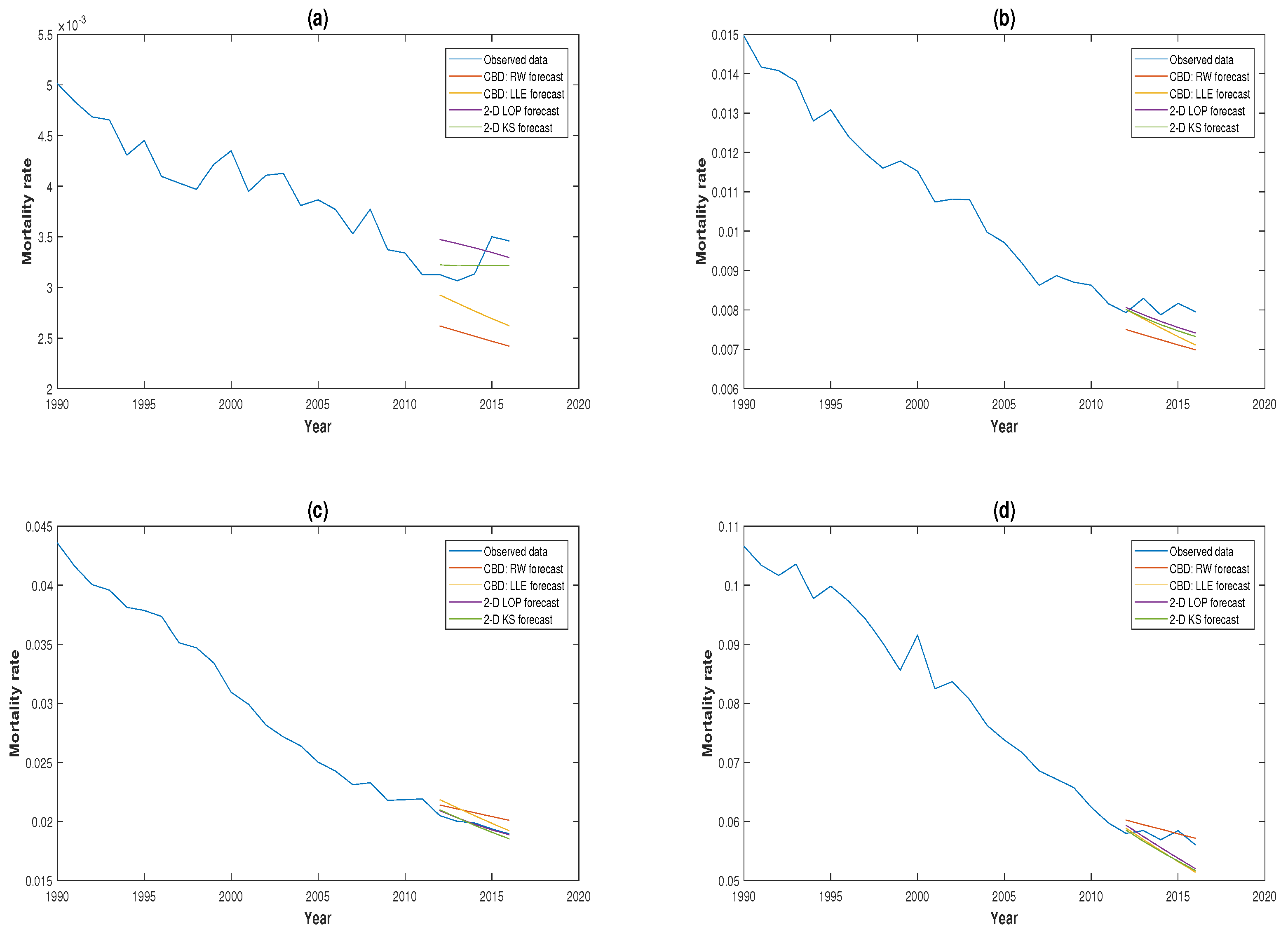
A comparison of the 3-, 5- and 10-year-ahead mortality forecasts for the four models against the real mortality experience for GB males aged 50, 60, 70 and 80 is illustrated in Figure 2, Figure 3 and Figure 4. It can be seen from these plots that the 2D KS model outperformed the other three models in the majority of circumstances. This is consistent with the conclusions we drew earlier based on the statistical measures.

3.4. Robustness of Projections

It has been claimed that in some cases, mortality forecast can be sensitive to the length of historical data employed in the modelling process (Denuit and Goderniaux 2005). According to Cairns et al. (2011), the robustness of the forecast relative to the sample period used to calibrate the model is one of the desirable properties of mortality models. Therefore, in this section, we examine the robustness of forecast for all four models by changing the starting time of the investigation period to 1970. Same backtesting techniques have been applied, and comparison and comments are made based on the differences in forecasting results. Mortality data during 1970–2013, 1970–2011 and 1970–2006 are used to generate the 3-, 5- and 10-year-ahead out-of-sample forecasts, respectively. We illustrate the results in

Table 4. Forecasting results of the CBD model for GB males aged 50–89 based on mortality data since 1970.

	CBD Model: RW Forecast			CBD Model: LLE Forecast
Forecast horizon	$E1(\%)$	$E2(\%)$	$E3(\%)$	$E1(\%)$	$E2(\%)$	$E3(\%)$
3	$-5.43$	8.34	10.80	$-4.83$	7.11	8.73
5	$-6.33$	8.06	10.42	$-6.46$	7.04	9.10
10	$-3.02$	7.42	8.97	$-4.45$	6.94	9.52

and

Table 5. Forecasting results of the 2D LOP model and the 2D KS model for GB males aged 50–89 based on mortality data since 1970.

	2D LOP Model			2D KS Model
Forecast horizon	$E1(\%)$	$E2(\%)$	$E3(\%)$	$E1(\%)$	$E2(\%)$	$E3(\%)$
3	$-2.36$	3.70	4.50	$-0.61$	2.39	3.14
5	$-0.47$	4.64	5.76	$-3.59$	4.53	5.53
10	5.25	7.06	9.98	1.97	3.80	5.06

.

It can be seen from Table 4 that, for both the random walk approach and the local linear approach, the change in the length of historical data employed in estimation process seemed to have a minor influence on the mortality projection. Compared to Table 2, the differences in the short- and medium-term forecasting results were modest; while the results show that the 10-year-ahead mortality forecast for RW forecast improved when we truncated the period of historical data used. It is worthwhile to undertake some further research to investigate possible reasons for this finding. Further, it can be argued that the random walk approach is more exposed to the influence of changes in the length of historical data employed than the local linear approach. On the other hand, the local linear approach seemed to be more robust. This should be expected since the bandwidth selection in local linear approach gave more weight to recent mortality experience, and thus the method would be less affected by the change in starting time of the investigation. Overall, we conclude that both of the forecasting approaches to the CBD model appear to be relatively robust even if the local approach was better in this regard.

An important finding from the results in Table 5 is that the forecasting results from the 2D KS model remained unchanged when different historical data periods were used. As described in Section 2.3, the optimum bandwidths and correlation parameter were selected based on the out-of-sample forecasting performance of the model. Therefore, the validation dataset was still the same, and the bandwidths would still give more weight to the most recent mortality experience. This could possibly explain the reason why the forecasting results remained unchanged. In contrast, compared to Table 3, when we considered mortality data only after 1970, the medium- to long-term forecasting performance of the 2D LOP model improved. A possible explanation for this is that a structural break may have occurred in the 1970s, so including data before the break would potentially worsen the forecast ability of the model.

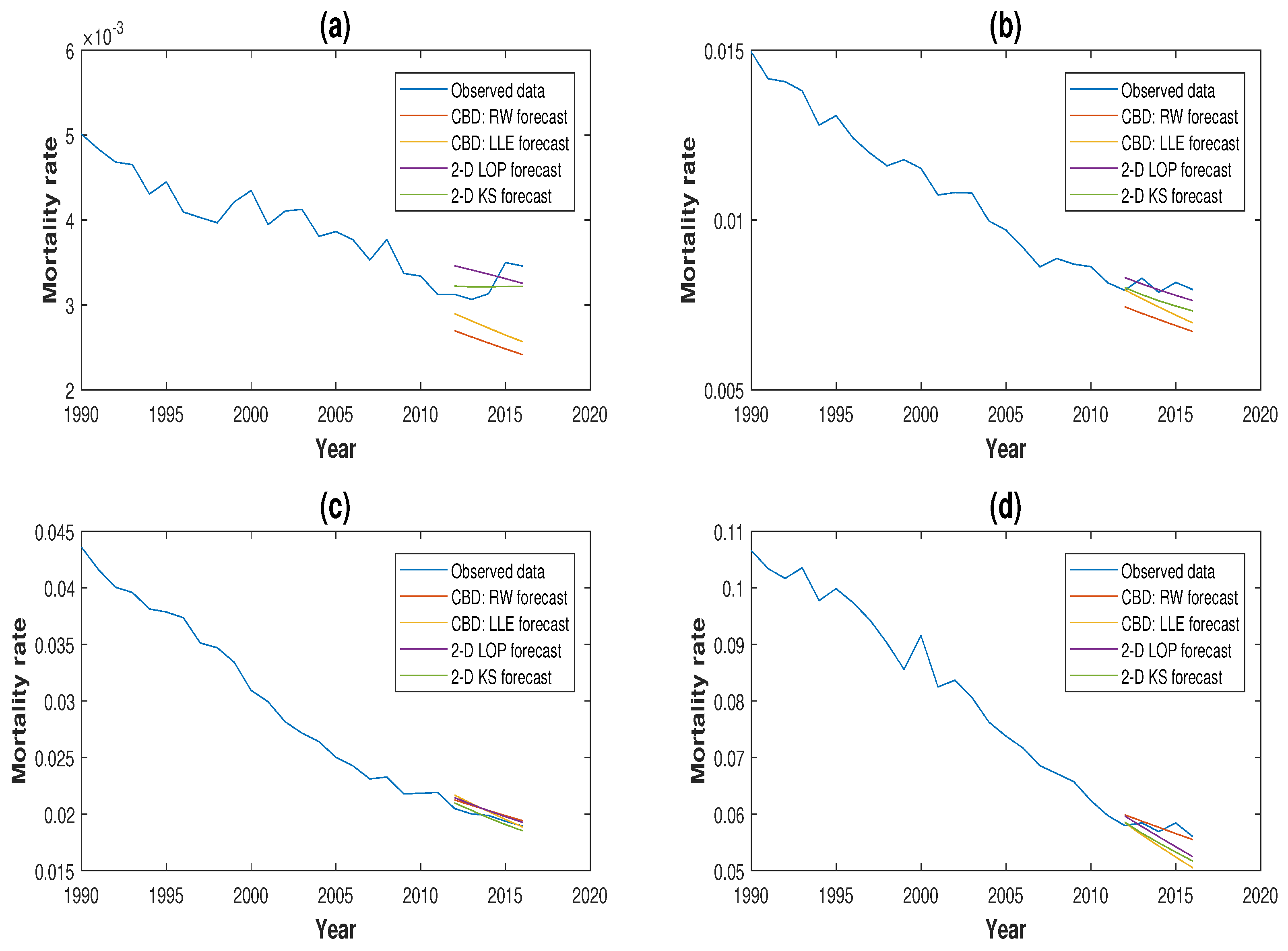
Our conclusions made in Section 3.3 on the preference of using local information in mortality projection still holds based on the results shown in Table 4 and Table 5 as the performances of local linear forecast and kernel smoothing forecast were still better than their comparators that used global information in the forecasting process. Moreover, it can also be concluded that the forecasts from the local approaches were more robust than the forecasts from the global approaches. Plots comparing the 3-, 5- and 10-year-ahead mortality forecasts for the four models for GB males aged 50, 60, 70 and 80 based on mortality experience from 1970 are illustrated in Figure 5, Figure 6 and Figure 7.

4. Conclusions

In this paper, we made a formal comparison between two sets of mortality models on their forecasting performance. The two models in each group had a similar design in their structure, but one projected future mortality rates using local information and the other global information. One main conclusion made from the case study conducted based on GB male mortality experience is that, in the forecasting process, local information seemed to have greater predictive power, and thus, it should be given more weight when doing future mortality projection. The study also included a test on the robustness of the forecast relative to different historical periods used in estimation. We conclude that overall, the four models included in the analysis have a satisfactory level of robustness and are suitable for the purpose of future mortality projection. However, local modelling does perform slightly better in this respect.

For future study, we can extend this work to include younger age groups by applying the local forecasting approach to a boarder range of models, such as the Lee–Carter model and the P-splines model Currie et al. (2004). Moreover, longer mortality datasets of high quality can also be considered, for example the Swedish mortality data.

References

- Booth, Heather, and Leonie Tickle. 2008. Mortality modelling and forecasting: A review of methods. Annals of Actuarial Science 3: 3–43. [Google Scholar] [CrossRef]
- Brouhns, Natacha, Michel Denuit, and Jeroen K. Vermunt. 2002. A Poisson log-bilinear approach to the construction of projected lifetables. Insurance: Mathematics and Economics 31: 373–93. [Google Scholar] [CrossRef]
- Cairns, Andrew J. G., David Blake, and Kevin Dowd. 2006. A two-factor model for stochastic mortality with parameter uncertainty: Theory and calibration. Journal of Risk and Insurance 73: 687–718. [Google Scholar] [CrossRef]
- Cairns, Andrew J. G., David Blake, Kevin Dowd, Guy D. Coughlan, David Epstein, Alen Ong, and Igor Balevich. 2009. A quantitative comparison of stochastic mortality models using data from England & Wales and the United States. North American Actuarial Journal 13: 1–35. [Google Scholar]
- Cairns, Andrew J. G., David Blake, Kevin Dowd, Guy D. Coughlan, David Epstein, and Marwa Khalaf-Allah. 2011. Mortality density forecasts: An analysis of six stochastic mortality models. Insurance: Mathematics and Economics 48: 355–67. [Google Scholar] [CrossRef]
- Currie, Iain D., Maria Durban, and Paul H. C. Eilers. 2004. Smoothing and forecasting mortality rates. Statistical Modeling 4: 279–98. [Google Scholar] [CrossRef]
- Denuit, Michel, and Anne-Cécile Goderniaux. 2005. Closing and projecting life tables using log-linear models. Bulletin of the Swiss Association of Actuaries 1: 29–48. [Google Scholar]
- Dickson, David C. M., Mary Hardy, and Howard R. Waters. 2009. Actuarial Mathematics for Life Contingent Risks. London: Cambridge University Press. [Google Scholar]
- Dokumentov, Alexander, and Rob J. Hyndman. 2014. Bivariate Data with Ridges: Two-Dimensional Smoothing of Mortality Rates. Working Paper Series; Melbourne: Monash University. [Google Scholar]
- Dowd, Kevin, Andrew J. G. Cairns, David Blake, Guy D. Coughlan, David Epstein, and Marwa Khalaf-Allah. 2010. Evaluating the goodness of fit of stochastic mortality models. Insurance: Mathematics and Economics 47: 255–65. [Google Scholar] [CrossRef]
- Gompertz, Benjamin. 1825. On the nature of the function expressive of the law of human mortality, and on a new mode of determining the value of life contingencies. Philosophical Transactions of the Royal Society 115: 513–85. [Google Scholar] [CrossRef]
- Härdle, Wolfgang. 1990. Applied Nonparametric Regression. London: Cambridge University Press. [Google Scholar]
- Haberman, Steven, and Arthur Renshaw. 2009. On age-period-cohort parametric mortality rate projections. Insurance: Mathematics and Economics 45: 255–70. [Google Scholar] [CrossRef]
- Human Mortality Database. 2019. University of California, Berkeley (USA), and Max Planck Institute for Demographic Research (Germany). Available online: http://www.mortality.org (accessed on 22 February 2019).
- Hyndman, Rob J., and Md Shahid Ullah. 2007. Robust forecasting of mortality and fertility rates a functional data approach. Computational Statistics & Data Analysis 51: 4942–56. [Google Scholar]
- Li, Han, Colin O’Hare, and Xibin Zhang. 2015. A semiparametric panel approach to mortality modelling. Insurance: Mathematics and Economics 61: 264–70. [Google Scholar]
- Li, Han, Colin O’Hare, and Farshid Vahid. 2016. Two-dimensional kernel smoothing of mortality surface: An evaluation of cohort strength. Journal of Forecasting 35: 553–63. [Google Scholar] [CrossRef]
- Li, Han, and Colin O’Hare. 2017. Semi-parametric extensions of the Cairns–Blake–Dowd model: A one-dimensional kernel smoothing approach. Insurance: Mathematics and Economics 77: 166–76. [Google Scholar] [CrossRef]
- Li, Han, Colin O’Hare, and Farshid Vahid. 2017. A flexible functional form approach to mortality modelling: Do we need additional cohort dummies? Journal of Forecasting 36: 357–67. [Google Scholar]
- Lee, Ronald D, and Lawrence R. Carter. 1992. Modeling and forecasting U.S. mortality. Journal of the American Statistical Association 87: 659–75. [Google Scholar] [CrossRef]
- Mádi-Nagy, Gergely. 2012. Polynomial bases on the numerical solution of the multivariate discrete moment problem. Annals Operations Research 200: 75–92. [Google Scholar] [CrossRef]
- O’Hare, Colin, and Youwei Li. 2012. Explaining young mortality. Insurance: Mathematics and Economics 50: 12–25. [Google Scholar] [CrossRef]
- Plat, Richard. 2009. On stochastic mortality modelling. Insurance: Mathematics and Economics 45: 393–404. [Google Scholar]