An Object-Oriented Bayesian Framework for the Detection of Market Drivers

Abstract

We use Object Oriented Bayesian Networks (OOBNs) to analyze complex ties in the equity market and to detect drivers for the Standard & Poor’s 500 (S&P 500) index. To such aim, we consider a vast number of indicators drawn from various investment areas (Value, Growth, Sentiment, Momentum, and Technical Analysis), and, with the aid of OOBNs, we study the role they played along time in influencing the dynamics of the S&P 500. Our results highlight that the centrality of the indicators varies in time, and offer a starting point for further inquiries devoted to combine OOBNs with trading platforms.

1. Introduction

Object Oriented Bayesian Networks—OOBNs—are hierarchical graphical models that break down the initial commitment into a set of sub-problems, and hence into subgraphs, encoding and representing the states of the world in a probabilistic fashion Koller and Pfeffer (1997). They are generally conceived as a robust alternative to Bayesian Networks (BNs) Pearl (1985): OOBNs, in fact, work best in integrating data from various sources and in considering information at different temporal or spatial resolutions Nagl et al. (2008); furthermore, they overcome several drawbacks of BNs Niedermayer (2008). In fact, BNs tend to perform poorly on high dimensional data Huang et al. (2013), Apollo (2017), and in practical applications BNs can suffer for overfitting Sun and Shenoy (2007). Moreover, it is possible to have more than a BN exactly representing the same joint probability distribution, but with a different direction for some of the edges, thus creating problems to assign the right direction of causation between edges Zhong and Xiao (2017).

Applications of OOBNs span over a variety of fields: from forensic genetics Dawid et al. (2007) to medical diagnosis Nagl et al. (2008), information fusion Sutton et al. (2004), and reliability analysis Langseth and Portinale (2007). However, the potential of OOBNs in finance is still rather unexplored: to the best of the authors’ knowledge, in fact, only Mortera et al. (2013) apply OOBNs to model anti-competitive behavior in the market, while Musella and Vicard (2015) analyzes improvement strategies in quality management and customer satisfaction.

Our work contributes to this research trail by illustrating a practical application of OOBNs on the Standard & Poor’s 500 (S&P 500) index, exploring the causal relationships between the S&P 500 and a bunch of heterogeneous drivers. The issue is part of a more general debate aimed at highlighting the role played by indicators of various nature on fluctuations of stocks and financial indexes; the problem has raised a big wave of essays so that it is not possible to mention everything; we therefore limit them to some of the most relevant. The seminal work of Fama et al. (1969), for instance, investigates the behavior of securities fluctuations depending on splits; later, Hillmer and Yu (1979) analyzes with a statistical method the market speed of adjustment to new information, while Chen et al. (1986) and Shanken and Weinstein (2006) examine a number of macro-economic variables and their influence on price fluctuations; furthermore, Mian and Sankaraguruswamy (2012) uses a measure of investor’s sentiment for evaluating how the stock price reacts to firm-specific news; finally, Gokmenoglu and Fazlollahi (2015) turn the attention on commodities’ persistence. The main point arising from this huge literature corpus is that the behavior of securities and financial indexes is the result of the interplay among very different variables.

Our research question concerns then disclosing how OOBNs can be helpful to detect main determinants of the S&P 500 index disentangling the complex ties among them and to suggest a trading behavior: we are going to show that OOBNs make possible representing in the same model aspects that should be generally hard to analyze with more conventional techniques and only at the cost of performing at the same time regressions, statistical analyses or information retrieved by data providers such as Bloomberg (https://www.bloomberg.com/), Factset (https://www.factset.com) or Datastream (https://infobase.thomsonreuters.com). Our conclusion is that the OOBN is a promising statistical technique because it allows for summarizing in a single tool the instances of various sophisticated investigation methods; moreover, it helps at highlighting the different influence of determinants across the years, working well as a thermometer of the investors’ attitude to trade on the market.

With respect to the existing literature, our work therefore contributes towards various aspects. First of all, for what pertains the combination between the technique in use and the addressed problem: OOBNs have been never applied to determine the drivers of a financial index, and a fortiori to develop signals for active trading. All in all, the added value of this research is not only in managing complexity and unveiling the determinants of a leading financial index, but also in suggesting a concrete way to address such amount of information towards a practical application.

In line with the above, the rest of the paper is organized as follows. Section 2 is devoted to illustrate materials and methods: it starts by describing the dataset to move then at illustrating basic definitions about Bayesian and Object-Oriented Bayesian Networks; Section 3 discusses the results, and Section 4 provides the conclusions.

2. Materials and Methods

2.1. Data

The S&P 500 is an American stock market index based on the market capitalization of 500 large companies whose common stock is listed on the NYSE (New York Stock Exchange, https://www.nyse.com/) or NASDAQ (National Association of Securities Dealers Automated Quotations, https://www.nasdaq.com/). It is a ratio opposing the sum of the adjusted market capitalization of 500 stocks with an index divisor, which is a proprietary figure developed by Standard & Poor’s:

$$\mathrm{S}\&\mathrm{P}500=\frac{{\displaystyle \sum _{k=1}^{500}AdjCa{p}_k}}{Div},$$

(1)

where $AdjCa{p}_k$, is the adjusted capitalization of the k-th stock ($k=1,\dots ,500$), and $Div$ is the divisor, which multiple sources1 peg at 8.9 billion, and it is adjusted in the case of stock issuance, mergers, change of companies in the S&P 500 amongst other corporate actions, thus ensuring that such events do not significantly alter the value of the index. The constituency and weighting methodology LLC (2013) make the S&P 500 index different from other US stock market indices; furthermore, due to the inclusion of companies which covers all areas of the United States and across all industries, it is generally considered an effective representation for the economy as well as a bellwether for the economy.

Provided the relevance of the index, we are aimed at capturing the most relevant ties among the S&P 500 and a bunch of indicators. In choosing them, we follow the approach proposed by Patel et al. (2011) that classifies indicators into a set of investment categories (Value, Growth, Sentiment and Momentum/Technical Analysis—TA) containing all the information needed for the analysis of a market index, both from a quantitative and a qualitative perspective. The complete listings with a short description are provided in

Table 1. Indicators list.

Name	Network ID	Investment Areas
		Growth	Value	Sentiment	Momentum and TA
Gold	GOLD	x
Unemployment rate	UNEMP	x
DXY index	DXY	x
Gross Domestic Product	GDP_G	x
Wheat	WHEAT	x
Crude oil	OIL	x
Copper	COPPER	x
Price to Cash Flow	PCF		x
Sales Growth	SALES${}_{\_}$G		x
EBITDA growth	EBITDA${}_{\_}$G		x
Enterprise Value to EBITDA	EV${}_{\_}$EBITDA		x
Price to Book Value	P${}_{\_}$BV		x
Price to Sales	P${}_{\_}$S		x
Earnings price per Share	EPS		x
EPS growth	EPS${}_{\_}$G		x
Dividend Yield	DVD${}_{\_}$YLD		x
Profit margin	PROFIT		x
Profit per Sale	PS		x
Return on Equity	ROE		x
Ebitda margin	EBITDA${}_{\_}$MRG		x
Implied Volatility in 52 weeks	VOLA52W			x
VIX	VIX			x
Relative Strength Index	RSI				x
Rate of change	ROC				x
20 and 50 Moving Average Cross	MA20${}_{\_}$50				x
Moving Average Convergence	MACD				x
Divergence

.

Table 1 shows for each indicator the abbreviation employed throughout the paper (Network ID), as well as the block (Investing Area) which the index belongs to (Growth, Value, Sentiment, Momentum and TA). We are also going to provide a short explanation for the variables (referred by their abbreviation) included into our study, divided by area.

Growth

GOLD is the most popular precious metal used as investment, especially in case of rising inflation; UNEMP represents the percentage of the total unemployed labor force actively looking for a job and willing to work. The DXY Index is the weighted geometric mean of the value of the US Dollar against the following currencies: Euro (57.6%), Yen (13.6%), Pound (11.9%), Canadian Dollar (9.1%), Swedish Krona (4.2%), and Swiss Franc (3.6%). GDP includes private and public consumption, government expenditure, investments and the trade balance; it is a measure of the economic activity in a country. WHEAT is an agricultural commodity generally used to hedge against inflation. OIL is an unrefined petroleum product whose price monitors the activity level in the manufacturing sector. COPPER is one of the most versatile industrial metals; cheaper than precious metals, it has wide application in various industries.

Value

All indicators in this investment area are ratios including weighted sums of variables in the financial statements of S&P 500 listed companies. Those variables include: the index level and cash flow (PCF); enterprise values and EBITDA (EV${}_{\_}$EBITDA); the index price level and book values (P${}_{\_}$BV); the index price level and sales (P${}_{\_}$S); dividends per share and the index price level (DVD${}_{\_}$YLD); net income and revenues (PROFIT); net income and net sales (PS); earnings and the total amount of shares outstanding in the index (EPS); net income and related shareholders’ equity (ROE); EBITDA and revenues (EBITDA${}_{\_}$MRG). Finally, PROFIT/EBITDA${}_{\_}$MRG/EPS${}_{\_}$G monitor the growth of these variables in neighbor periods.

Market Sentiment

VOLA52W is the annual implied volatility (derived from the options prices); VIX is the CBOE2 volatility index.

Momentum and Technical Analysis

RSI compares the magnitude of recent gains to recent losses. ROC measures the speed at which the index changes over a certain period. MA20${}_{\_}$50 considers crossing between a fast (20) and a slow (50) moving average. MACD3 is the difference between 12 and 26 weeks exponential moving averages, with the 9 weeks moving average as a trigger.

2.2. Preliminary Data Analysis

This study uses weekly data from the S&P 500 index in the period Jan 2000–March 2018, collected from the Bloomberg database.

To limit the influence of abrupt changes in the time series, we applied the Bai–Perron test Bai and Perron (2003) in search for structural breaks. The test assumes to consider a standard linear regression model $\mathcal{M}$:

$$y_t={\mathbf{x}}_t^{\prime }·\mathbf{b}+u_t,$$

(2)

where $y_t$ is the dependent variable, · is the dot–product operator, $\mathbf{b}$ and ${\mathbf{x}}_t$ are the regression coefficients and the regressors vectors, respectively, and $u_t$ the zero mean error term. The Bai–Perron technique checks whether it is reasonable to assume that the coefficients are not constant through time, as there are m breakpoints, where the coefficients shift from one stable regression relationship to a different one, so that (2) is turned into:

$$y_t={\mathbf{x}}_t^{\prime }·{\mathbf{b}}_i^0+u_t,t=T_{i-1}^0+1\dots ,T_i^0,$$

(3)

for $i=1,\dots ,m+1$, while $T_0^0=0$ and $T_{m+1}^0=T$, with T being the total sample size.

The number of breakpoints is not exogenously given, but it is estimated via a double–check procedure at first aimed at minimizing the Residual Sum of Squares (RSS):

$${\displaystyle \mathrm{RSS}(T_1,\dots ,T_m)=\sum _{j=1}^{m}RS{S}_j(T_1,\dots ,T_m),}$$

(4)

with:

$${\displaystyle RS{S}_j(T_1,\dots ,T_m)=\sum _{t=T_{j-1}+1}^{T_j}{\left\{y_t-{\mathbf{x}}_t^{\prime }·\widehat{\beta }{\left(\left\{{\widehat{T}}_i\right\}\right)}_{i=1}^m\right\}}^2,}$$

(5)

where $\widehat{\beta }\left(\left\{{\widehat{T}}_i\right\}\right)$ denotes the estimates based on the given m-partition $(T_1,\dots ,T_m)$. The reliability of the number m of breaks is then checked by minimizing the Bayesian Information Criterion (BIC) of M Schwarz (1978):

$$\mathrm{BIC}=klnT-2ln\widehat{L},$$

(6)

where $\widehat{L}=p\left(y\right|\widehat{\vartheta },M)$ is the value of the likelihood function of the model $\mathcal{M}$, with parameters $\widehat{\vartheta }$ for the observed time series y; T is the sample size and k is the number of parameters estimated by the model.

Table 2. RSS and BIC scores for the Bai–Perron test.

	$\mathit{m}=0$	$\mathit{m}=1$	$\mathit{m}=2$	$\mathit{m}=3$
RSS	118,462,323	30,094,169	26,358,449	23,555,096
BIC	13,040	11,834	11,730	11,643

shows the RSS and the BIC associated to the number of breakpoints m varying from 0 to 3; a visual inspection is also provided in Figure 1: all the computations have been done within the R4 framework using the library strucchange.

We highlight preliminarily that the existence of structural breaks was monitored obeying to various instances. From one hand, in fact, we are aware of considering a time frame (from 2000 to 2018) with various changes in the market dynamics, induced by events such as the 9/11 facts, the subprime crisis, the Lehman Brothers default, to give some examples. However, we also agree with the position of the econometrician Rob J. Hyndman5 claiming that, in general, it is better talking about evolutionary changes, which can be misidentified as structural changes due to the use of these tests. Overall, these considerations led us to set at $m=3$ the maximum number of breakpoints to test for, as an acceptable compromise between the need of documenting abrupt changes in the dynamics of the observed time series and the need of avoiding misapplication errors.

The lowest values of both the RSS and BIC correspond to $m=3$, thus suggesting the presence of three breaks and hence four regimes, as highlighted in Figure 2 representing the behavior of the S&P 500 from January 2000 to March 2018 with breaks evidenced by vertical dashed lines.

These conclusions are also supported by the values in

Table 3. Regression coefficients with three breakpoints: the label *** indicates significance of the test values at the 99% level of confidence.

	Estimate	Std. Error	t-Value	$\mathit{Pr}(>|\mathit{t}\left|\right)$
Intercept	7.0269	0.0089	790.648	$<2\times {10}^{-16}$ ***
segment2	0.0917	0.0112	8.177	$8.92\times {10}^{-16}$ ***
segment3	0.5204	0.0146	35.741	$<2\times {10}^{-16}$ ***
segment4	0.7667	0.0147	52.211	$<2\times {10}^{-16}$ ***

showing the significance at the 99% confidence level of the regression coefficients on the S&P 500 assuming the existence of four segments of the data, corresponding to the breaks identified by the Bai–Perron procedure.

Breaks correspond to the beginning of years 2004, 2009 and to the ending of 2013. We divided our dataset accordingly: basic statistics for each period are reported in

Table 4. Main statistics for the observed block on the S&P 500.

Time-Slice	ID	First	End	Length	Mean	Median	Min	Max	Std	1st Q	3rd Q
2000–2004	TS1	03/01/00	02/02/04	215	1145.0989	1125.1700	800.5800	1527.4599	201.2463	988.8201	1316.8900
2004–2009	TS2	09/02/04	16/03/09	267	1251.6363	1261.4899	683.3800	1561.8000	176.3480	1161.5150	1387.0599
2009–2013	TS3	23/03/09	16/12/13	248	1295.5064	1287.0899	815.9400	1818.3199	228.7867	1116.9075	1414.6950
2013–2018	TS4	23/12/13	19/03/18	222	2165.6753	2092.2600	1782.589	2872.8701	249.4976	1990.3999	2347.5125

. In detail, we show for each time-slice the reference id (ID), the initial and final date (First and End), the length of the block of data, and a set of basic statistics: Mean, Median, Minimum (Min) and Maximum (Max) values observed in the period, Standard deviation (Std), first and third quantile (1stQ, 3rdQ).

The values in Table 4 combined to the graphical inspection of the index (see Figure 2) suggest the existence of up and down phases in the S&P 500. The challenge we are going to address is testing to which extent the OOBN is helpful at $\left(i\right)$ correctly identifying them and $\left(ii\right)$ develop trading suggestions towards the right direction, i.e., buying when an uptrend starts, selling when prices begin to slow down, or maintain the position when the price moves up and down without a leading direction (sideward movements)

2.3. Methodology

The Bayesian Network (BN) is a valuable tool in constructing and understanding relations among elements of a problem under uncertainty; however, there can be situations where its use can be impractical or even ineffective: we have already highlighted in Section 1 that this can be the case of complex problems, involving too many variables, as well as when it is necessary to represent a hierarchy of dependencies. This is typical for time series models where a certain structure is replicated over time so that links between random variables in different time slices are established.

Going to the heart of the issue, our research question involves all the underlined aspects, as we consider twenty-six variables which potentially can influence the S&P 500 (complexity) whose behavior can be mutually affected (hierarchical effect); furthermore, the S&P index varies over time (time-slice effect). In the paper, we discuss how to overcome these issues with the aid of Object Oriented Bayesian Networks (OOBNs).

We want also to point out that the proposed application of the OOBN within the financial context is not a mere exercise in style, but it is fully justified as in the specialized literature Benjamin-Fink and Reilly (2017) OOBNs are claimed capable to analyze the following scenarios: $\left(i\right)$ known hierarchy and full observability, $\left(ii\right)$ known hierarchy and partial observability, $\left(iii\right)$ unknown hierarchy and full observability, or $\left(iv\right)$ unknown hierarchy and partial observability. The discussed application falls in case $\left(iii\right)$ and thus it makes appropriate referring to the OOBN. Nevertheless, BNs and OOBNs are strictly related. An OOBN acts as a meta-network linking a number of BNs.

From a formal viewpoint, a BN is a a Directed Acyclic Graph (DAG) with nodes representing random variables and arcs expressing the probabilistic dependencies between variables. A BN is therefore fully described by the following elements:

-

the graph structure $\mathcal{G}=(\mathcal{V},\mathcal{E})$, where $\mathcal{V}=\{v_1,v_2,\dots ,v_n\}$ is the set of vertexes, and $\mathcal{E}$ is the set of directed edges;

-

a finite probability space $(\mathsf{\Omega },\mathcal{A},\mathcal{P})$, where $\mathsf{\Omega }$ is the probability space, $\mathcal{A}$ is a $\sigma$-algebra on $\mathsf{\Omega }$ and $\mathcal{P}$ a measure on $\mathsf{\Omega }$, such that: $\mathcal{P}\left(\mathsf{\Omega }\right)=1$; $\mathcal{P}(\varnothing )=0$, and $\mathcal{P}\left(A\right)\le \mathcal{P}\left(B\right)$, if $A\subseteq B$;

-

a set of random variables defined on $(\mathsf{\Omega },\mathcal{A},\mathcal{P})$, one for each node of the graph whose conditional probability distributions express the strengths of dependency relations between the random variable and its parent connection on the graph:

$${\displaystyle p(v_1,v_2,\dots ,v_n)=\prod _{k=1}^{n}p\left(v_k\right|\mathcal{G}\left(v_k\right)).}$$

(7)

In this way, it is possible to define for the graph a set of Conditional Probability Tables (CPT) representing the mutual relationships between nodes and parent nodes. Nodes without any parent have a very simple CPT, given by the prior probability distribution of the node itself. In the remaining cases, the CPT represents all the node’s joint probability, as given in (7).

An example of CPT is provided in

Table 5. Joint probability distribution for two variables x and y that can assume three states: 0, 1 and 2.

	$\mathit{x}=0$	$\mathit{x}=1$	$\mathit{x}=2$	$\mathit{P}\left(\mathit{y}\right)$
$y=0$	1/11	1/11	2/11	4/11
$y=1$	2/11	1/11	1/11	4/11
$y=2$	1/11	1/11	1/11	3/11
$P\left(x\right)$	4/11	3/11	4/11	1

and

Table 6. Conditional Probability Table for two variables x and y that can assume three states: 0, 1 and 2.

	$\mathit{x}=0$	$\mathit{x}=1$	$\mathit{x}=2$
$P(y=0|x)$	1/4	1/3	2/4
$P(y=1|x)$	2/4	1/3	1/4
$P(y=2|x)$	1/4	1/3	1/4
Sum	1	1	1

, where we examine the case of two variables x and y that can assume three states: 0, 1, and 2.

The cells show the probability of a particular combination of x and y values. The first column sum is the marginal probability that $x=0$. If we want to find the probability that $y=0$ given that $x=0$, we must compute: $1/11÷4/11=1/4$. Likewise, from the same column, we can compute the probability that $y=1$ when $x=0$, that is: $2/11÷4/11=1/2$, and the probability that $y=2$ when $x=0$: $1/11÷4/11=1/4$. Working in a similar way with the piece of information in the third and fourth column, we can also find the conditional probabilities for y equalling 0; 1 and given that $x=1$ and $x=2$, respectively. The result is the table of conditional probabilities for y, provided in Table 6.

With respect to the BN formalism, OOBNs go one step further. The rationale of the OOBN resides in decomposing the complex problem into simpler sub-problems (classes) that can be modeled via BNs linked one to each other into an upper hierarchical structure. The transfer of information is enabled by inference nodes which form interface nodes. Every BN fragments serves as a class, while fragments resulting from instantiating these classes are named objects Nielsen and Jensen (2007). With respect to the BN, then, the OOBN offers a richer paradigm.

An example of an OOBN based on Langseth and Nielsen (2003) is presented in Figure 3.

The model introduces six classes: Insurance, Theft, Accident, Car, Car owner and Driver, which can be seen as describing different (abstract) entities in the domain. For instance, the class Car describes the properties associated with a car; the nodes Cushioning, Mileage, CarValue, RuggedAuto and Antilock are the nodes also used outside the class hence, they occur as output nodes, whereas Vehicle year and Make model are input nodes and Airbag is a normal node. In a similar fashion, the class Driver models the driving features of a car owner. In the insurance context, driving characteristics are an integral part of the notion of a car owner and an instantiation of Driver is therefore encapsulated in the class CarOwner. The class Insurance encapsulates the corresponding instantiations of the other classes. It is worth noticing the active use of reference links: for example, there are two CarValue nodes in the OOBN: C.CarValue is defined in C:Car, but as C.CarValue is a parent of T.Theft, it is imported into T:Theft using an input node (which is named T.CarValue). The reference link between these two nodes shows that it is the same random variable that is used in both situations.

Training an OOBN is typically divided into two distinct stages. The first stage creates the structure of the network: the hierarchical structure maximizing the data likelihood is usually drawn with the Chow–Liu procedure Chow and Liu (1968), while the NPC algorithm Steck (2001) helps in limiting inconsistencies among the set of conditional independence and dependence statements derived from the dataset and in choosing the most suitable model for the problem. The model construction is completed by estimating the conditional probability tables from the data with the EM (Expectation–Maximization) algorithm Lauritzen (1996). More details about the EM algorithms are provided in Appendix A.

3. Simulation and Results

3.1. Experiment Design

For each time-slice, we used earlier 90% of the data to build the OOBN, while the remaining 10% was used later to test the derived trading signals. Labels, first and ending together with the length of each block of data are reported in

Table 7. Labels and length of each block of data employed in the trials.

ID	First	End	Length (in Weeks)
$L-T{S}_1$	03/01/00	01/09/03	215
$T-T{S}_1$	08/09/03	02/02/04	21
$L-T{S}_2$	09/02/04	01/09/08	240
$T-T{S}_2$	08/09/08	16/03/09	27
$L-T{S}_3$	23/03/09	17/06/13	223
$T-T{S}_3$	24/06/13	16/12/13	25
$L-T{S}_4$	23/12/13	09/10/17	200
$T-T{S}_4$	16/10/17	19/03/18	22

.

For the examined data, we alternated between two stages: OOBN learning (OOBN-L), in which an OOBN is built based on the twenty-six indicators described in Section 2, and OOBN towards trading (OOBN-T), in which the probability derived in the first stage is employed to develop a trading signal. The steps of the procedure are described in the following rows: note that Steps 3 and 4 were done using the Hugin Expert software6, any other computation was done using R (version 3.5.2, R Development Core Team, GPL license) and Microsoft Excel (version 2018).

• Set $i=1$.
• Select $L-T{S}_i$.
• (OOBN–L) Build the OOBN using the Chow–Liu procedure combined to the NPC algorithm.
• (OOBN–L) Derive the CPT for each node with the EM procedure and the related probability for the S&P 500 of going up (1), down (2) or side-ward (0) and extract the highest.
• (OOBN-L) If the highest probability for the S&P 500 is associated to the up state, then put the signal $s_t=1$ and buy; if highest probability for the S&P 500 is associated to the down state, then set $s_t=-1$ and sell; otherwise, set $s_t=0$ and maintain the position.
• (OOBN-T) Select $T-T{S}_i$ and compute the time-series of log-returns:

  $$r_k=log{p}_{k+1}-log{p}_k,$$

  (8)

  for $k=1,\dots ,n-1$, where n is the length of $T-T{S}_i$.
• (OOBN-T) For each price level in $T-T{S}_i$:

  (a) 

  Evaluate:

  $$s_t\times r_k.$$

  (9)

  (b) 

  Compute the sign of (9):

  $$sg{n}_k=signum(s_t\times r_k).$$

  (10)

  (c) 

  Compute:

  $${\widehat{r}}_k=sg{n}_k{r}_k.$$

  (11)

• (OOBN-T) With the time series: ${\widehat{T-TS}}_i=\left\{{\widehat{r}}_k\right\}$ check the goodness of the trading signals with the bundle of performance measures provided in

  Table 8. Indicators employed to evaluate the performance of the trading signals.

  Performance Measure	Abbreviation	Formula
  % Correct Directional Change	%CDC	${\displaystyle \%CDC=\frac{1}{\nu -1}\sum _{k=1}^{\nu }{\mathbf{1}}_k}$
  Annualized return	AR	${\displaystyle AR=52\times \frac{1}{\nu -1}\sum _{k=1}^{\nu }{\widehat{r}}_k}$
  Annualized volatility	AV	$AV=\sqrt{52}\sqrt{{\displaystyle \frac{1}{\nu -1}\sum _{k=1}^{\nu }{({\widehat{r}}_k-\widehat{\mu })}^2}}$
  Sharpe Ratio	SR	$SR=AR/AV$
  Number of Up periods	NUP	$NUP=card\{{\widehat{r}}_k>0\}$
  Number of Down periods	ND	$ND=card\{{\widehat{r}}_k\le 0\}$
  Average gain in up periods	AG	${\displaystyle AG=\frac{1}{NUP}\sum _{k=1}^{\nu }{\mathbf{1}}_k\times r_k}$
  Average loss in down periods	AL	${\displaystyle AL=\frac{1}{ND}\sum _{k=1}^{\nu }(1-{\mathbf{1}}_k)\times r_k}$
  Average gain/loss ratio	AGL	$AGL=AG/AL$

  .
• Set $i=i+1$ and go to Step 2.

Table 8 shows the performance measures used to asses the goodness of the trading signals in each period. Their selection is driven by the choices documented in Dempster et al. (2001) and Resta (2009). To ease the readability of the table, please note that all the performance measures assume working on time-series of length $\nu =n-1$ whose corresponding mean value is denoted by $\widehat{\mu }$; when necessary, it has been made use of the indicator function:

$${\mathbf{1}}_k=\left\{\begin{array}{cc}\hfill 1,& r_k\times {\widehat{r}}_k>0,\hfill \\ \hfill 0,& r_k\times {\widehat{r}}_k\le 0.\hfill \end{array}\right.$$

(12)

Finally, the annualisation factor is set equal 52, as we are working with weekly observations.

3.2. Discussion

Every computation was made within the Windows environment on an Intel i7 processor. The computational time spent by the Hugin Expert software in developing each OOBN in the paper is equal on average to six minutes and includes maximizing the data likelihood with the Chow–Liu procedure and the NPC algorithm to limit inconsistencies among the set of conditional independence and dependence statements and estimating the conditional probability tables from the data with the EM algorithm. However evaluating the efficiency of the procedure as well as discussing the computational complexity of the OOBN go beyond the scopes of the paper. The interested reader can refer to more specialized texts in literature, such as: Liu et al. (2016) and Galia (2004).

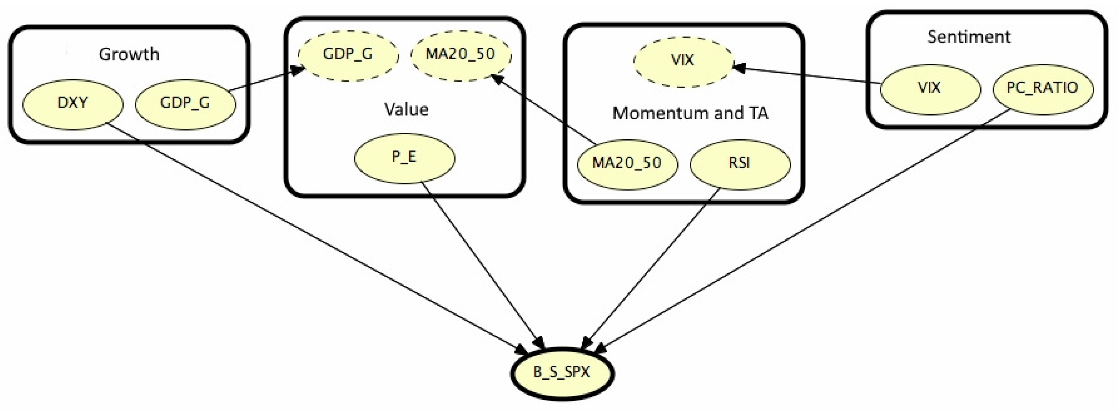
Moving to the discussion, Figure 4 visualizes the results for the first time segment, illustrating its meaning and relevance: comments on the OOBN refer to $L-T{S}_1$, while remarks on the trading signal refer to $T-T{S}_1$. Similar considerations apply for other examined periods so that the conclusion we draw now can be extended to them in a straightforward manner.

From Figure 4, we may see as $B_{\_}{S}_{\_}SPX$ is conditioned by four instance nodes belonging to the classes indicated in Section 2; in detail, the output nodes are: DXY (Growth), P${}_{\_}$E (Value), RSI (Momentum and TA) and PC${}_{\_}$Ratio (Sentiment). Besides Growth and Value classes communicate via the node $GD{P}_{\_}G$ that is a parent node within the Value class; MA20${}_{\_}$50 is the bridge between Value and Momentum/TA, which in turn is connected to the Sentiment group by the VIX.

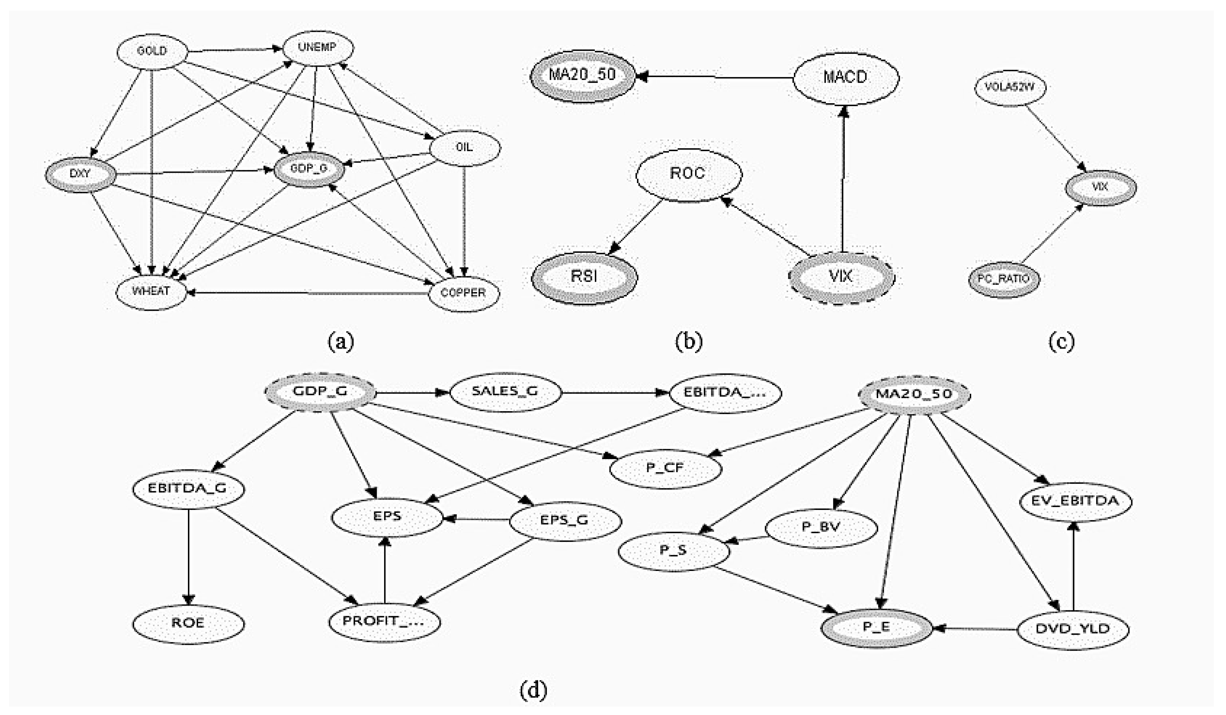
From this representation, one can appreciate the simplicity of the final hierarchy that hides the intricacy of ties existing among the variables: Figure 5 unveils the structure of these complex relationships for each object.

From Figure 5, we observe that there is a BN inside each class of the OOBN presented in Figure 4. Analyzing the ties inside of those BNs, it is possible to get additional insights about the final aspect of the OOBN. To motivate this assertion, we discuss the case of the BN inside the Growth class: clearly similar considerations can be extended to the other classes. More in detail, the behavior of GOLD directly affects all the nodes in the Growth class (Figure 5a), while the opposite happens to WHEAT that is directly conditioned by any node inside the class. Other big influencers are DXY and OIL, directly insisting on four over six nodes of the class; among the greatest followers, on the other hand, we find COPPER and $GD{P}_G$ on which insist five on six nodes. The fact that DXY is an instance node in the OOBN in Figure 4 is probably due to the sensitivity in changes of the other nodes in the class, as shown in Figure 6 with the aid of tornado plots comparing the relative importance of the class nodes. In detail, we simulate the sensitivity of each variable to a $\pm 20\%$ change in the values of the remaining ones, putting them in order from the highest to the lowest response. To make an example, looking at Figure 6a, we may observe the response of $GD{P}_G$ with respect to $\pm 20\%$ fluctuations of the other variables, appearing on the left–hand side of the plot: the sensitivity is at the highest level with DXY; nevertheless, it is maintained at high level also with respect to changes in the variables UNEMP, OIL, GOLD and COPPER, while it is notably lower with WHEAT. Similar considerations can be applied to the other tornado plots.

Moreover, in the light of the results in Figure 5 and Figure 6, the driving role of DXY with respect to the S&P 500 becomes more understandable.

Overall, disclosed information is multipurpose. First, it aids at revealing the hierarchy of ties in the market in a very simplified way: the main point is that, from the set of dependency among 26 indicators, we extract only four output nodes driving the index. This has notable implications when deriving the CPT for the S&P 500, as it is necessary to address $4\times 3$ instead of $26\times 3$ probabilities for each state.

Furthermore, with respect to the remarks done for the Growth class, we have also highlighted the existence of a richest network of relations behind those drivers. Second, we are going to show that this information can be managed to operate buy/sell/neutral actions on the S&P 500, and hence to simulate the impact on the index of changes in its drivers.

Table 9. Relations among instance nodes and S&P 500 during the four regimes. The bottom row shows the overall impact on the S&P 500. Numbers code the behavior in the market: In-Trend (1), Reversal (2), and Sideward (0). Corresponding probability is given between brackets.

	$\mathit{L}-{\mathit{TS}}_1$	$\mathit{L}-{\mathit{TS}}_2$	$\mathit{L}-{\mathit{TS}}_3$	$\mathit{L}-{\mathit{TS}}_4$
DXY	1	1	2	1
	(46.15)	(42.48)	(38.76)	(40.73)
P${}_{\_}$E	2	1	1	1
	(51.39)	(38.14)	(35.83)	(37.06)
RSI	1	1	2	1
	(39.68)	(48.10)	(41.15)	(41.76)
PC${}_{\_}$Ratio	1	2	1	2
	(41.35)	(39.66)	(43.36)	(40.59)
Overall	1	2	1	2
	(38.12)	(42.93)	(43.09)	(43.49)

examines the role of outputs on the S&P 500 in the four regimes and adds some clues to understand the overall direction of the index, as explained in previous rows. Here, the dependency structure for the S&P 500 index ($B_{\_}{S}_{\_}SPX$) is built under the rationale that the drivers should move either towards the same direction or not, thus suggesting an overall direction of the index, coded by numbers: In-trend (1), Reversal (2) or Sideward (0). In more detail, In-trend is connected to a bullish stage, with increasing price levels from a week to another; the opposite happens in the presence of Reversal, while Sideward is generally associated with uncertainty in the market, with prices moving in a lateral fashion, i.e., sometimes up and sometimes down, without any defined trend.

The overall impact of the drivers varies in time. During the first period, three output nodes on four agree in suggesting an in-trend position (1). Moving from the first to the second period, we have again three indicators over four aligned towards in-trend, but the final decision is for a Reversal (2), this, in our opinion, testifying the major influence of the PC${}_{\_}$Ratio over the remaining indexes. The same occurs in the fourth regime. The situation in the third regime is different from other ones, as we have two drivers suggesting to stay in-trend and two indicating the opposite. In this perfect balancing situation, the final decision (1) is kept according to the suggestions of Value and Sentiment indicators. These remarks therefore suggest the prominent role played by Sentiment indicators.

To support these conclusions, we examined the performance of a trading system inspired by the results discussed in Table 9, through the trail described in Section 3.1. Results are reported in

Table 10. Performance values of the trading signals in the test datasets.

Performance Measure	$\mathit{T}-{\mathit{TS}}_1$	$\mathit{T}-{\mathit{TS}}_2$	$\mathit{T}-{\mathit{TS}}_3$	$\mathit{T}-{\mathit{TS}}_4$
%CDC	0.8421	0.4	0.7391	0.7
AR	0.2148	0.4409	0.1912	0.2139
AV	0.0283	0.1113	0.0280	0.0385
SR	7.5949	3.9609	6.8179	5.558
NUP	16	10	17	14
ND	4	16	7	7
AG	0.0052	0.022	0.0052	0.0062
AL	0.0082	0.0205	0.0049	0.0082
AGL	0.6321	1.0749	1.0562	0.7505

.

The results in Table 10 highlight a very good performance of the trading system based on the OOBNs: with the exception of $T-T{S}_2$, in fact, the %CDC is sensitively over 60%, with peaks over 80% in the case of $T-T{S}_1$. Indeed, the performance of all the indicators are aligned to %CDC and confirm the satisfactory behavior of the trading system. A possible explanation for the results in the second testing period can be probably retrieved in observing that $T-T{S}_2$ includes weeks where the 2008 financial crisis was at its very blooming stage. The Average Volatilty (AV) values seem supporting this conclusion.

Furthermore, we provided in

Table 11. Comparison of the performance among the Buy and Hold (B&H), the Näive and the OOBN-based (OOBN-b) strategies.

	B&H	Näive	OOBN-b
$T-T{S}_1$	1.0507	1.0507	1.0858
$T-T{S}_2$	0.7989	1.2208	1.2418
$T-T{S}_3$	1.0548	1.0548	1.0919
$T-T{S}_4$	1.0283	0.9707	1.0897

the comparison of the performance among the Buy and Hold (B&H), the näive and (Näive) and the OOBN-based (OOBN-b) strategies. B&H is a passive investment strategy for which the investor buys stocks and holds them for the whole period regardless of fluctuations in the market with no concern for short-term price movements and technical indicators. The Näive is a strategy assuming to buy in uptrend periods and to sell during downtrends. The performance was computed as:

$${\displaystyle perf=\prod _{k=1}^{\nu }(1+r_k{|}_{strategy}).}$$

(13)

Here, $r_k{|}_{strategy}$ is the log-return $r_k$ in the B&H case, while we have $r_k{|}_{strategy}={\widehat{r}}_k$ as defined in (11) for the OOBN-b; finally, when dealing with the näive strategy, it is: $r_k{|}_{strategy}=1+r_k$ during uptrend periods and $r_k{|}_{strategy}=1+(-1)r_k$ when the time series goes downtrend. In practice, (13) evaluates the convenience of investing each unit capital at the rate $r_k{|}_{strategy}$ for each week of the testing period.

We can note that the performance of the OOBN-b strategy is always higher than both the B&H and the Näive. This is true also during the downtrend periods $T-T{S}_2$ and $T-T{S}_4$ when B&H and Näive, respectively, poorly performed. This evidence then supports the idea that the OOBN can be successfully combined with trading systems.

4. Conclusions

The study shows how Object-Oriented Bayesian Networks (OOBNs) can be employed to combine both qualitative and quantitative information of the market and to manage a large amount of information. Our results give an insight about the evolution of the market in a quite simplified way despite of the complexity of ties behind. In addition, our results open the room for a general remark and three interesting scenarios. For what concerns the remark, we have observed the mutant role of the indicators, although, in the examined cases, the Sentiment driver seems playing a prominent role in influencing the overall behavior of the S&P 500. Turning to the scenarios, the probability associated with each state makes it possible to develop what-if cases, as discussed in our results; moreover, the interplay among output nodes and the S&P 500 suggests the possibility of developing trading systems based on the OOBNs responses. To conclude, the use of dedicated software, such as Hugin Expert, which is able to manage both discrete and continuous variables, makes room enough to further developments, such as including a larger variety of explicative variables to refine both the technique and the overall results.

References

- Apollo, Magdalena. 2017. Prognostic and diagnostic capabilities of OOBN in assessing investment risk of complex construction projects. Procedia Engineering 196: 236–43. [Google Scholar] [CrossRef]
- Bai, Jushan, and Pierre Perron. 2003. Computation and analysis of multiple structural change models. Journal of Applied Econometrics 18: 1–22. [Google Scholar] [CrossRef] [Green Version]
- Benjamin-Fink, Nicole, and Brian K. Reilly. 2017. A road map for developing and applying objec-oriented bayesian networks to “WICKED”problems. Ecological Modelling 360: 27–44. [Google Scholar] [CrossRef]
- Chen, Nai-Fu, Richard Roll, and Stephen A. Ross. 1986. Economic forces and the stock market. The Journal of Business 59: 83–403. [Google Scholar] [CrossRef]
- Chow, C., and Cong Liu. 1968. Approximating discrete probability distributions with dependence trees. IEEE Transactions on Information Theory 14: 462–67. [Google Scholar] [CrossRef]
- Dawid, A. Philip, Julia Mortera, and Paola Vicard. 2007. Object-Oriented Bayesian Networks for Complex Forensic DNA Profiling Problems. Forensic Science International 169: 195–205. [Google Scholar] [CrossRef]
- Dempster, Michael, Tom W. Payne, Yazann Romahi, and G. W. P. Thompson. 2001. Computational learning techniques for intraday FX trading using popular technical indicators. IEEE Transactions on Neural Networks 12: 744–54. [Google Scholar] [CrossRef]
- Fama, Eugene F., Lawrence Fisher, Michael C. Jensen, and Richard Roll. 1969. The Adjustment of Stock Prices to New Information. International Economic Review 10: 1–21. [Google Scholar] [CrossRef]
- Galia, Weidl. 2004. Adaptive risk assessment in complex large scale processes with reduced computational complexity. Paper presented at 9th International Conference on Industrial Engineering Theory, Applications & Practice, Auckland, New Zealand, November 27–30. [Google Scholar]
- Gokmenoglu, Korhan K., and Negar Fazlollahi. 2015. The Interactions among Gold, Oil, and Stock Market: Evidence from S&P500. Procedia Economics and Finance 25: 478–88. [Google Scholar]
- Hillmer, Steven C., and P. L. Yu. 1979. The market speed of adjustment to new information. Journal of Financial Economics 7: 321–45. [Google Scholar] [CrossRef]
- Huang, Shuai, Jing Li, Jieping Ye, Adam Fleisher, Kewei Chen, Teresa Wu, and Eric Reiman. 2013. A Sparse Structure Learning Algorithm for Gaussian Bayesian Network Identification from High-Dimensional Data. IEEE Transactions on Pattern Analysis and Machine Intelligence 35: 1328–42. [Google Scholar] [CrossRef] [PubMed]
- Koller, Daphne, and Avi Pfeffer. 1997. Object-Oriented Bayesian Networks. Paper presented at Thirteenth Conference on Uncertainty in Artificial Intelligence (UAI ’97), Providence, RI, USA, August 1–3; pp. 302–13. [Google Scholar]
- Langseth, Helge, and Thomas D. Nielsen. 2003. Fusion of Domain Knowledge with Data for Structural Learning in Object Oriented Domains. Journal of Machine Learning Research 4: 339–68. [Google Scholar]
- Langseth, Helge, and Luigi Portinale. 2007. Bayesian networks with applications in reliability analysis. In Bayesian Network Technologies: Applications and Graphical Models. Hershey: IGI Global, pp. 84–102. [Google Scholar]
- Lauritzen, Steffen L. 1996. Graphical Models. Wotton-under-Edge: Clarendon Press. [Google Scholar]
- Liu, Quan, Ayeley Tchangani, and François Peres. 2016. Modelling complex large scale systems using object oriented Bayesian networks (OOBN). IFAC-PapersOnLine 49: 127–32. [Google Scholar] [CrossRef]
- Standard & Poor’s Financial Services LLC staff. 2013. S&P Indices Index Mathematics Methodology. New York: The McGraw-Hill Companies, Inc. [Google Scholar]
- Mian, G. Mujtaba, and Srinivasan Sankaraguruswamy. 2012. Investor Sentiment and Stock Market Response to Earnings News. The Accounting Review 87: 1357–84. [Google Scholar] [CrossRef]
- Mortera, Julia, Paola Vicard, and Cecilia Vergari. 2013. Object-Oriented Bayesian Networks for a decision support system for antitrust enforcement. The Annals of Applied Statistics 7: 714–38. [Google Scholar] [CrossRef]
- Musella, Flaminia, and Paola Vicard. 2015. Object-oriented Bayesian networks for complex quality management problems. Quality & Quantity 49: 115–33. [Google Scholar]
- Nagl Sylvia, Matt Williams, and Jon Williamson. 2008. Objective Bayesian Nets for Systems Modelling and Prognosis in Breast Cancer. In Innovations in Bayesian Networks. New York: Springer International, pp. 131–67. [Google Scholar]
- Niedermayer, Daryle. 2008. An Introduction to Bayesian Networks and Their Contemporary Applications. In Innovations in Bayesian Networks-Theory and Applications. New York: Springer International, vol. 156, pp. 117–30. [Google Scholar]
- Nielsen, Thomas Dyhre, and Finn V. Jensen. 2007. Bayesian Networks and Decision Graphs. New York: Springer. [Google Scholar]
- Patel, Pankaj, Souheang Yao, Ryan Carlson, Abhra Banerji, and Joseph Handelman. 2011. Quantitative Research—A Disciplined Approach. Technical Report. Zurich: Credit Suisse Equity Research. [Google Scholar]
- Pearl, Judea. 1985. Bayesian Networks: A Model of Self-Activated Memory for Evidential Reasoning. Paper presented at 7th Conference of the Cognitive Science Society, Irvine, CA, USA, August 15–17; pp. 329–34. [Google Scholar]
- Resta, Marina. 2009. Seize the (intra)day: Features selection and rules extraction for tradings on high-frequency data. Neurocomputing 72: 3413–27. [Google Scholar] [CrossRef]
- Schwarz, Gideon. 1978. Estimating the dimension of a model. Annals of Statistics 6: 461–64. [Google Scholar] [CrossRef]
- Shanken, Jay, and Mark I. Weinstein. 2006. Economic forces and the stock market revisited. Journal of Empirical Finance 13: 129–44. [Google Scholar] [CrossRef]
- Steck, Harald. 2001. Constrained—Based Structural Learning in Bayesian Networks Using Finite Data Sets. Ph.D. thesis, Technical University Munich, Munich, Germany. [Google Scholar]
- Sun, Lili, and Prakash P. Shenoy. 2007. Using Bayesian networks for bankruptcy prediction: Some methodological issues. European Journal of Operational Research 180: 738–53. [Google Scholar] [CrossRef]
- Sutton, Charles, Clayton T. Morrison, Paul R. Cohen, Joshua Moody, and Jafar Adibi. 2004. A Bayesian Blackboard for Information Fusion. Technical Report. Amherst: Department of Computer Science, Massachusetts University. [Google Scholar]
- Zhong, Hongye, and Jitian Xiao. 2017. Enhancing Health Risk Prediction with Deep Learning on Big Data and Revised Fusion Node Paradigm. Scientific Programming 2017: 1901876. [Google Scholar] [CrossRef]