Model Efficiency and Uncertainty in Quantile Estimation of Loss Severity Distributions

Abstract

Quantiles of probability distributions play a central role in the definition of risk measures (e.g., value-at-risk, conditional tail expectation) which in turn are used to capture the riskiness of the distribution tail. Estimates of risk measures are needed in many practical situations such as in pricing of extreme events, developing reserve estimates, designing risk transfer strategies, and allocating capital. In this paper, we present the empirical nonparametric and two types of parametric estimators of quantiles at various levels. For parametric estimation, we employ the maximum likelihood and percentile-matching approaches. Asymptotic distributions of all the estimators under consideration are derived when data are left-truncated and right-censored, which is a typical loss variable modification in insurance. Then, we construct relative efficiency curves (REC) for all the parametric estimators. Specific examples of such curves are provided for exponential and single-parameter Pareto distributions for a few data truncation and censoring cases. Additionally, using simulated data we examine how wrong quantile estimates can be when one makes incorrect modeling assumptions. The numerical analysis is also supplemented with standard model diagnostics and validation (e.g., quantile-quantile plots, goodness-of-fit tests, information criteria) and presents an example of when those methods can mislead the decision maker. These findings pave the way for further work on RECs with potential for them being developed into an effective diagnostic tool in this context.

1. Introduction

Quantiles of probability distributions play a central role in the definition of risk measures (e.g., value-at-risk, conditional tail expectation) which in turn are used to capture the riskiness of the distribution tail. Estimates of risk measures are needed in many practical situations such as in pricing of extreme events, developing reserve estimates, designing risk transfer strategies, and allocating capital. When solving such problems, the first highly consequential task is to find point estimates of quantiles and to assess their variability. In this context, the empirical nonparametric approach is the simplest one to use (see Jones and Zitikis 2003), but it lacks efficiency due to the scarcity of sample data in the tails. On the other hand, parametric estimators can significantly improve quantile estimators’ efficiency (see Brazauskas and Kaiser 2004; Kaiser and Brazauskas 2006). Moreover, the parametric approach can accommodate truncation and censoring that are common features of insurance loss data. Of course, the main drawback of parametric estimators is that they are sensitive to initial modeling assumptions, which creates model uncertainty1.

There is a growing number of studies on various aspects of model risk in modeling, measuring and pricing risks. Cairns (2000) was the first author to systematically study model risk in insurance. He discussed different sources of model risk, including parameter uncertainty and model uncertainty, and presented methods to treat these uncertainties coherently. Hartman et al. (2017) focused on parameter uncertainty and analyzed its impact in different sectors of insurance practice, namely, life insurance, health insurance, and property/casualty insurance. They also gave a comprehensive review of the literature concerning parameter uncertainty. A recent article by Hong et al. (2018) shows typical claim predictions change when the model is uncertain. In particular, they illustrate such effects by using standard model selection tools such as Akaike Information Criterion to determine the “best” regression subset of covariates, and then apply the selected model for claim prediction. Bignozzi et al. (2015) and Samanthi et al. (2017) are two recent examples of theoretical and practical investigations, respectively, of the effects of the data dependence assumption on subsequent risk measuring. Also, an extensive simulation study involving estimation of upper quantiles of lognormal, log-logistic, and log-double exponential distributions under model and parameter uncertainty was conducted by Modarres et al. (2002). Their overall conclusion was that when modeling is done by assuming one of the three families and treating the other two as possible misspecification, the least severe effect on upper quantile estimates occurs when the lognormal distribution is assumed.

Further, there is even more interest in this topic in the financial risk management literature. Model uncertainty within the risk aggregation problems has been recently studied by Embrechts et al. (2015) and Cambou and Filipović (2017), and for value-at-risk estimation by Alexander and Sarabia (2012). Cont et al. (2010) and Glasserman and Xu (2014) linked financial risk measurement procedures, model risk, and robustness. The first paper suggests the use of the classical robust statistics techniques for managing model risk, while the second pursues model distance and entropy based techniques to derive the worst-case risk measurements (relative to measurements from a baseline model). Finally, Aggarwal et al. (2016) and Black et al. (2018) provide comprehensive accounts on model risk identification, measurement, and management in practice. These authors develop a model risk framework, identify distinct model cultures within an organization, review common methods and challenges for quantifying model risk, and discuss difficulties that arise in mapping model errors to actual financial impact.

The implied conclusion in many academic and practice oriented papers on model risk is that it can be reduced or mitigated by using all or a combination of the following: performing model validation, fitting multiple models, and applying various stress tests or sensitivity analysis. This idea was in part adopted in the case studies of Brazauskas and Kleefeld (2016), which were based on well-known (real) reinsurance data. What was discovered by these authors, however, is that fitting multiple models and using extensive model validation for each of them may not be sufficient if data are left-truncated. That is, they used quantile-quantile plots, Kolmogorov-Smirnov (KS) and Anderson-Darling (AD) tests, Akaike and Bayesian information criteria (AIC and BIC) and had concluded that six different models are acceptable for each of the 12 data sets analyzed. However, when all those models were used to estimate the 90% and 95% quantiles (value-at-risk measures) for ground-up loss, for some data sets they resulted in similar estimates, which would be expected, while for others they were far apart, which is counterintuitive. Moreover, using left-truncated operational risk data, Yu and Brazauskas (2017) have shown that even shifted parametric models (which might seem like a plausible option but nonetheless incorrectly account for data truncation) can pass those standard model validation tests. Next, due to the presence of deductibles and policy limits in insurance contracts, data truncation and censoring are unavoidable modifications of the loss severity variable. This suggests that quantile and, more generally, risk measure estimation requires careful thinking and analysis.

In this paper, we present the empirical nonparametric, maximum likelihood, and percentile-matching estimators of ground-up loss distribution quantiles (at various levels). Asymptotic distributions of these estimators are derived when data are left-truncated and right-censored. Relative efficiency curves (REC) for all the estimators are then constructed, and plots of such curves are provided for exponential and single-parameter Pareto distributions. Then, we generate a sample of 50 observations from a left-truncated and right-censored Pareto I model and using that data set investigate how biased quantile estimates can be when one makes incorrect distributional assumptions or relies on a wrong modeling approach. The numerical analysis is also supplemented with standard model diagnostics and validation (e.g., quantile-quantile plots and KS and AD tests) and demonstrates how those methods can mislead the decision maker. In addition, we examine the information provided by RECs and conclude that such curves have strong potential for being developed into an effective diagnostic tool in this context.

The rest of the paper is organized as follows. In Section 2, nonparametric and parametric quantile estimators are defined and their asymptotic distributions are specified when the underlying random variable is left-truncated and right-censored. The next section presents two illustrative examples of RECs for exponential and single-parameter Pareto distributions. Specifically, RECs of maximum likelihood, percentile matching, and empirical estimators of quantiles of these distributions are plotted. Section 4 studies the effects of distribution choice and modeling approach on estimates of quantiles. Concluding remarks are offered in Section 5. Finally, the appendix provides two asymptotic theorems of mathematical statistics and a detailed description of how to contruct RECs. These results are essential to analytic derivations in the paper, and we recommend the reader to review them first.

2. Quantile Estimation

Insurance contracts have coverage modifications that need to be taken into account when modeling the underlying loss severity variable. In this section, we specify the estimators of quantiles of the ground-up distribution and derive their asymptotic distributions when the loss variable is affected by left truncation (due to deductible) and right censoring (due to policy limit). We consider three types of estimators: empirical (Section 2.1), aximum likelihood, MLE (Section 2.2), and percentile matching, PM (Section 2.3).

To present the estimators and their properties, let us start with notation and assumptions. Suppose we observe n continuous independent identically distributed (i.i.d.) random variables $X_1^{*},\dots ,X_n^{*}$, where each $X^{*}$ is equal to the ground-up variable X, if X exceeds threshold t ($t\ge 0$) but is capped at upper limit u ($u>t$). That is, $X^{*}$ is a mixed discrete-continuous random variable that satisfies the following conditional event relationship:

$$X^{*}\stackrel{d}{=}min\{X,u\}|X>t,$$

where $\stackrel{d}{=}$ denotes “equal in distribution.” Also, let us denote the probability density function (pdf), cumulative distribution function (cdf), and quantile function (qf) of X as f, F, and $F^{-1}$, respectively. Then, the cdf $F_{*}$, pdf $f_{*}$, qf $F_{*}^{-1}$ of $X^{*}$ are related to F, f, $F^{-1}$ and given by:

$$F_{*}\left(x^{*}\right|t;u)=\left\{\begin{array}{cc}0,& x^{*}\le t;\\ \frac{F\left(x^{*}\right)-F\left(t\right)}{1-F\left(t\right)},& t<x^{*}<u;\\ 1,& x^{*}\ge u,\end{array}\right.$$

(1)

$$f_{*}\left(x^{*}\right|t;u)=\left\{\begin{array}{cc}\frac{f\left(x^{*}\right)}{1-F\left(t\right)},& t<x^{*}<u;\\ \frac{1-F\left(u^{-}\right)}{1-F\left(t\right)},& x^{*}=u;\\ 0,& elsewhere,\end{array}\right.$$

(2)

$$F_{*}^{-1}\left(s\right|t;u)=\left\{\begin{array}{cc}{F}^{-1}\left(s+(1-s)F\left(t\right)\right),& 0\le s<\frac{F\left(u\right)-F\left(t\right)}{1-F\left(t\right)};\\ u,& \frac{F\left(u\right)-F\left(t\right)}{1-F\left(t\right)}\le s\le 1.\end{array}\right.$$

(3)

Note that we are interested in estimating the pth quantile of X (i.e., $F^{-1}\left(p\right)$) based on the observed data $X_1^{*}=x_1^{*},\dots ,X_n^{*}=x_n^{*}$. Thus, Theorems A1 and A2 in Appendix A.1 and the REC construction of Appendix A.2 have to be applied to functions (1)–(3), not F, f, $F^{-1}$.

2.1. Empirical Approach

As mentioned earlier, the empirical approach is restricted to the range of observed data. Indeed, based on $x_1^{*},\dots ,x_n^{*}$, the empirical estimator ${\widehat{F}}_{\mathrm{EMP}}\left(t\right)=0$. Thus, it cannot take full advantage of formulas (1)–(3), and yields a biased estimator that works within a limited range of quantile levels. In this case, the $F^{-1}\left(p\right)$ estimator is ${\widehat{F}}_{\mathrm{EMP}}^{-1}\left(p\right)=x_{(\lceil np\rceil )}^{*}<u$, and as follows from Theorem A1,

$${\widehat{F}}_{\mathrm{EMP}}^{-1}\left(p\right)is\mathcal{AN}\left(F_{*}^{-1}\left(p\right),\frac{1}{n}\frac{p(1-p)}{f_{*}^2\left(F_{*}^{-1}\left(p\right)\right)}\right),0<p<\frac{F\left(u\right)-F\left(t\right)}{1-F\left(t\right)}.$$

(4)

To see that this estimator is positively biased, i.e., any (estimable) quantile of the observable variable $X^{*}$ is never below the corresponding quantile of the unobservable variable X (which is what we want to estimate), notice that for the mean parameter in (4), we have

$$F_{*}^{-1}\left(p\right)=F^{-1}\left(p+(1-p)F\left(t\right)\right)\ge F^{-1}\left(p\right),0<p<\frac{F\left(u\right)-F\left(t\right)}{1-F\left(t\right)},$$

with the inequality being strict unless $F\left(t\right)=0$. The inequality holds because $F^{-1}$ is strictly increasing (loss severities are non-negative absolutely continuous random variables) and $(1-p)F\left(t\right)\ge 0$.

2.2. MLE Approach

Parametric methods use the observed data $x_1^{*},\dots ,x_n^{*}$ and fully recognize its distributional properties. The MLE approach is one of the most common estimation techniques. It takes into account (1)–(3) and finds parameter estimates by maximizing the following log-likelihood function:

$$\begin{array}{c}log\mathcal{L}\left(\mathit{\theta }|x_1^{*},\dots ,x_n^{*}\right)=log\left[\prod _{i=1}^n{f}_{*}\left(x_i^{*}\right|t;u)\right]=log\left[\prod _{i=1}^n{\left[\frac{f\left(x_i^{*}\right)}{1-F\left(t\right)}\right]}^{\mathbf{1}\{t<x_i^{*}<u\}}{\left[\frac{1-F\left(u^{-}\right)}{1-F\left(t\right)}\right]}^{\mathbf{1}\{x_i^{*}=u\}}\right]\end{array}=\sum _{i=1}^{n}log\left[f\left(x_i^{*}\right)\right]\mathbf{1}\{t<x_i^{*}<u\}-nlog\left[1-F\left(t\right)\right]+log\left[1-F\left(u^{-}\right)\right]\sum _{i=1}^n\mathbf{1}\{x_i^{*}=u\},$$

(5)

where $\mathbf{1}\left\{\right\}$ denotes the indicator function.

Once parameter MLEs, ${\widehat{\theta }}_1,\dots ,{\widehat{\theta }}_k$, are available, the pth quantile estimate is found by plugging those MLE values into the parametric expression of $F^{-1}\left(p\right)=h({\theta }_1,\dots ,{\theta }_k)$. Let us denote this estimator as ${\widehat{F}}_{\mathrm{MLE}}^{-1}\left(p\right)=h({\widehat{\theta }}_1,\dots ,{\widehat{\theta }}_k)$. Then, as follows from the MLE’s asymptotic distribution and the delta method,

$${\widehat{F}}_{\mathrm{MLE}}^{-1}\left(p\right)is\mathcal{AN}\left(F^{-1}\left(p\right),\frac{1}{n}{\mathbf{d}}_{\mathbf{\theta }}{\mathbf{I}}_{\mathbf{\theta }}^{-\mathbf{1}}{\mathbf{d}}_{\mathbf{\theta }}^{\prime }\right),0<p<1,$$

(6)

where ${\mathit{d}}_{\mathit{\theta }}=\left(\partial h/\partial {\widehat{\theta }}_1,\dots ,\partial h/\partial {\widehat{\theta }}_k\right){|}_{({\theta }_1,\dots ,{\theta }_k)}$, and the entries of ${\mathit{I}}_{\mathit{\theta }}$ are given by (A7) with g replaced by (2). Note that (6) is defined for $0<p<1$, while (4) for $0<p<\frac{F\left(u\right)-F\left(t\right)}{1-F\left(t\right)}\le 1$.

2.3. PM Approach

A popular alternative to the MLE approach for estimation of loss distribution parameters is percentile matching (PM). To estimate k unknown parameters with the PM method and using the ordered data $x_{\left(1\right)}^{*}\le \cdots \le x_{\left(n\right)}^{*}$, one has to solve the following system of equations with respect to ${\theta }_1,\dots ,{\theta }_k$:

$$F_{*}^{-1}\left(p_1\right)=x_{\left(\lceil n{p}_1\rceil \right)}^{*},F_{*}^{-1}\left(p_2\right)=x_{\left(\lceil n{p}_2\rceil \right)}^{*},\dots ,F_{*}^{-1}\left(p_k\right)=x_{\left(\lceil n{p}_k\rceil \right)}^{*},$$

where $p_1<\cdots <p_k<\frac{F\left(u\right)-F\left(t\right)}{1-F\left(t\right)}$ and $x_{\left(\lceil n{p}_k\rceil \right)}^{*}<u$. Once parameter PMs, ${\tilde{\theta }}_1,\dots ,{\tilde{\theta }}_k$, are available, the pth quantile estimate is found by plugging those PM values into $F^{-1}\left(p\right)=h({\theta }_1,\dots ,{\theta }_k)$. Let us denote this estimator as ${\widehat{F}}_{\mathrm{PM}}^{-1}\left(p\right)=h({\tilde{\theta }}_1,\dots ,{\tilde{\theta }}_k)$. Then, as follows from Theorem A2 and the delta method,

$${\widehat{F}}_{\mathrm{PM}}^{-1}\left(p\right)is\mathcal{AN}\left(F^{-1}\left(p\right),\frac{1}{n}{\mathbf{d}}_{\mathbf{\theta }}{\mathbf{D}}_{\mathbf{\theta }}^{*}{\mathbf{\Sigma }}_{\mathbf{\theta }}{\left({\mathbf{D}}_{\mathbf{\theta }}^{*}\right)}^{\prime }{\mathbf{d}}_{\mathbf{\theta }}^{\prime }\right),0<p<1,$$

(7)

where ${\mathit{d}}_{\mathit{\theta }}=\left(\partial h/\partial {\tilde{\theta }}_1,\dots ,\partial h/\partial {\tilde{\theta }}_k\right){|}_{({\theta }_1,\dots ,{\theta }_k)}$ and ${\mathit{D}}_{\mathit{\theta }}^{*}$ is specified in Theorem A2. The entries of ${\mathbf{\Sigma }}_{\mathit{\theta }}$ are given by (A1) with g and $G^{-1}$ replaced by expressions (2) and (3), respectively. Note that (7) is defined for $0<p<1$, while (4) for $0<p<\frac{F\left(u\right)-F\left(t\right)}{1-F\left(t\right)}\le 1$.

3. RECs for Exponential and Pareto Models

In this section, we provide examples of RECs for exponential and single-parameter Pareto distributions under several data-truncation and censoring scenarios. For each model, we choose the (biased) empirical estimator of $F^{-1}\left(p\right)$ as the benchmark estimator. Then, using formulas (4), (6), and (7), we evaluate ${\mathrm{ARE}}_p$’s for the MLE and PM estimators with respect to the empirical estimator, as well as ${\mathrm{ARE}}_p$ of PM with respect to MLE. The three definitions of ${\mathrm{ARE}}_p$’s are given by Equations (A8)–(A10)

3.1. Exponential Distribution

Let $X_1,X_2,\dots$ be i.i.d. exponentially distributed random variables with cdf $F\left(x\right)=1-e^{-(x-x_0)/\theta },x\ge x_0$, pdf $f\left(x\right)=(1/\theta )e^{-(x-x_0)/\theta },x>x_0$, and qf $F^{-1}\left(s\right)=x_0-\theta log(1-s),0\le s\le 1$, and where $x_0\ge 0$ is known and $\theta >0$ is an unknown scale parameter. According to the model setup of Section 2, however, the $X_i$’s are unobservable. The data are generated by variables $X_1^{*},\dots ,X_n^{*}$ which are i.i.d. with cdf, pdf, and qf given by (1), (2), and (3), respectively. This implies that when $X_i$’s are exponentially distributed, we have

$$F_{*}\left(x^{*}\right|t;u)=\left\{\begin{array}{cc}0,& x^{*}\le t;\\ 1-e^{-(x^{*}-t)/\theta },& t<x^{*}<u;\\ 1,& x^{*}\ge u,\end{array}\right.$$

$$f_{*}\left(x^{*}\right|t;u)=\left\{\begin{array}{cc}(1/\theta )e^{-(x^{*}-t)/\theta },& t<x^{*}<u;\\ e^{-(u-t)/\theta },& x^{*}=u;\\ 0,& \mathrm{elsewhere},\end{array}\right.$$

$$F_{*}^{-1}\left(s\right|t;u)=\left\{\begin{array}{cc}-\theta log(1-s)+t,& 0\le s<1-e^{-(u-t)/\theta };\\ u,& 1-e^{-(u-t)/\theta }\le s\le 1.\end{array}\right.$$

Now, for the empirical estimator ${\widehat{F}}_{\mathrm{EMP}}^{-1}\left(p\right)=x_{(\lceil np\rceil )}^{*}$, the asymptotic result (4) becomes

$${\widehat{F}}_{\mathrm{EMP}}^{-1}\left(p\right)is\mathcal{AN}\left(-\theta log(1-p)+t,\frac{{\theta }^2}{n}\frac{p}{1-p}\right),0<p<1-e^{-(u-t)/\theta }.$$

(8)

The statement (8) shows that the asymptotic bias of ${\widehat{F}}_{\mathrm{EMP}}^{-1}\left(p\right)$ is $t-x_0$.

Further, MLE of $\theta$ is found by maximizing the log-likelihood (5) which in this case is

$$log\mathcal{L}\left(\theta |x_1^{*},\dots ,x_n^{*}\right)=-log\theta \sum _{i=1}^n\mathbf{1}\{t<x_i^{*}<u\}-\frac{1}{\theta }\sum _{i=1}^n\left[(x_i^{*}-t)\mathbf{1}\{t<x_i^{*}<u\}+(u-t)\mathbf{1}\{x_i^{*}=u\}\right].$$

It yields a closed-form solution for $\theta$:

$${\widehat{\theta }}_{\mathrm{MLE}}=\frac{{\sum }_{i=1}^n\left[(x_i^{*}-t)\mathbf{1}\{t<x_i^{*}<u\}+(u-t)\mathbf{1}\{x_i^{*}=u\}\right]}{{\sum }_{i=1}^n\mathbf{1}\{t<x_i^{*}<u\}}.$$

This in turn implies that ${\widehat{F}}_{\mathrm{MLE}}^{-1}\left(p\right)=x_0-{\widehat{\theta }}_{\mathrm{MLE}}log(1-p)$, and the asymptotic result (6) becomes

$${\widehat{F}}_{\mathrm{MLE}}^{-1}\left(p\right)is\mathcal{AN}\left(x_0-\theta log(1-p),\frac{{\theta }^2}{n}\frac{{log}^2(1-p)}{1-e^{-(u-t)/\theta }}\right),0<p<1.$$

(9)

Furthermore, since for the exponential distribution there is only one unknown parameter $\theta$, its PM estimator is derived by solving a single equation, $F_{*}^{-1}\left(p_1\right)=x_{\left(\lceil n{p}_1\rceil \right)}^{*}$. Note that $p_1$ has to be chosen from the range $0<p_1<1-e^{-(u-t)/\theta }$ (equivalently, $x_{\left(\lceil n{p}_1\rceil \right)}^{*}<u$). In this case, the resulting estimator is also explicit and given by

$${\widehat{\theta }}_{\mathrm{PM}}=\frac{t-x_{\left(\lceil n{p}_1\rceil \right)}^{*}}{log(1-p_1)}.$$

Subsequently, ${\widehat{F}}_{\mathrm{PM}}^{-1}\left(p\right)=x_0-{\widehat{\theta }}_{\mathrm{PM}}log(1-p)$, and the asymptotic result (7) becomes

$${\widehat{F}}_{\mathrm{PM}}^{-1}\left(p\right)is\mathcal{AN}\left(x_0-\theta log(1-p),\frac{{\theta }^2}{n}\frac{p_1}{1-p_1}{\left[\frac{log(1-p)}{log(1-p_1)}\right]}^2\right),0<p<1.$$

(10)

Finally, we have everything in place for computation of ARE${}_p$. Since ${\widehat{F}}_{\mathrm{EMP}}^{-1}\left(p\right)$ is our benchmark estimator which is biased, formulas (A8) and (A9) will be modified by replacing estimators’ variances with their mean-square errors (MSE). The MSE ratios based on (8)–(10) are:

$$\mathrm{ARE}\left({\widehat{F}}_{\mathrm{MLE}}^{-1}\left(p\right),{\widehat{F}}_{\mathrm{EMP}}^{-1}\left(p\right)\right)=\frac{\frac{{\theta }^2}{n}\frac{p}{1-p}+{(t-x_0)}^2}{\frac{{\theta }^2}{n}\frac{{log}^2(1-p)}{1-e^{-(u-t)/\theta }}},0<p<1-e^{-(u-t)/\theta },$$

(11)

$$\mathrm{ARE}\left({\widehat{F}}_{\mathrm{PM}}^{-1}\left(p\right),{\widehat{F}}_{\mathrm{EMP}}^{-1}\left(p\right)\right)=\frac{\frac{{\theta }^2}{n}\frac{p}{1-p}+{(t-x_0)}^2}{\frac{{\theta }^2}{n}\frac{{log}^2(1-p)}{{log}^2(1-p_1)}\frac{p_1}{1-p_1}},0<p<1-e^{-(u-t)/\theta },$$

(12)

$$\mathrm{ARE}\left({\widehat{F}}_{\mathrm{PM}}^{-1}\left(p\right),{\widehat{F}}_{\mathrm{MLE}}^{-1}\left(p\right)\right)=\frac{\frac{{\theta }^2}{n}\frac{{log}^2(1-p)}{1-e^{-(u-t)/\theta }}}{\frac{{\theta }^2}{n}\frac{{log}^2(1-p)}{{log}^2(1-p_1)}\frac{p_1}{1-p_1}}=\frac{(1-p_1){log}^2(1-p_1)}{p_1(1-e^{-(u-t)/\theta })},0<p<1.$$

(13)

Note that for $p\ge 1-e^{-(u-t)/\theta }$, the ratios (11) and (12) are infinite because ${\widehat{F}}_{\mathrm{EMP}}^{-1}\left(p\right)$ is undefined. Also, in (13), the probability level $p_1$ has to be chosen from the range $0<p_1<1-e^{-(u-t)/\theta }$.

In Figure 1, RECs of quantile estimators of the exponential ($x_0=100,\theta$) distribution are plotted for the left-truncation level $t=500$ and right-censoring at $u=2500$. In the first column of plots, the distribution is lighter tailed ($\theta =250$) with $F\left(t\right)=0.7981$, $F\left(u\right)=0.9999$, and $F_{*}\left(u\right|t;u)=0.9995$. In the second column of plots, the distribution has a heavier tail ($\theta =500$) with $F\left(t\right)=0.5507$, $F\left(u\right)=0.9918$, and $F_{*}\left(u\right|t;u)=0.9817$. Due to the high bias of the empirical estimator (which goes to ∞ as $p\to 0$), the vertical axes are plotted on the logarithmic scale to minimize visual distortions. Comparison of plots across the rows reveals a couple of patterns: first, in the top row it is clearly visible that a combination of heavier tail and a slightly smaller percentage of actually observed data $F_{*}\left(u\right|t;u)$ shifts all curves significantly upward (especially for small p); second, as is evident from all plots, the efficiency of PM estimators increases monotonically for $0<p_1<0.80$ and then starts to decrease for $0.80<p_1<1$ (i.e., the curves pm${}_4$ are above those of pm${}_3$ which are above pm${}_2$, etc., but pm${}_6$ are below pm${}_5$). Thus the $p_1\approx 0.80$ level is optimal for PM estimation. This fact is in agreement with the complete sample optimality result (see discussion in Section 3.1 of Brazauskas (2009)).

3.2. Pareto Distribution

Let $X_1,X_2,\dots$ be i.i.d. random variables distributed according to a single-parameter Pareto distribution with cdf $F\left(x\right)=1-{(x_0/x)}^{\alpha },x>x_0$, pdf $f\left(x\right)=(\alpha /x_0){(x_0/x)}^{\alpha +1},x>x_0$, and qf $F^{-1}\left(s\right)=x_0{(1-s)}^{-1/\alpha },0\le s\le 1$. Here $x_0>0$ is known and $\alpha >0$ is an unknown shape parameter, thus justifying the single-parameter characterization. As before, $X_i$’s are unobservable and the data are generated by variables $X_1^{*},\dots ,X_n^{*}$ which are i.i.d. with cdf, pdf, and qf given by (1), (2), and (3), respectively. This implies that when $X_i$’s are Pareto distributed, we have

$$F_{*}\left(x^{*}\right|t;u)=\left\{\begin{array}{cc}0,& x^{*}\le t;\\ 1-{(t/x^{*})}^{\alpha },& t<x^{*}<u;\\ 1,& x^{*}\ge u,\end{array}\right.$$

$$f_{*}\left(x^{*}\right|t;u)=\left\{\begin{array}{cc}(\alpha /t){(t/x^{*})}^{\alpha +1},& t<x^{*}<u;\\ {(t/u)}^{\alpha },& x^{*}=u;\\ 0,& \mathrm{elsewhere},\end{array}\right.$$

$$F_{*}^{-1}\left(s\right|t;u)=\left\{\begin{array}{cc}t{(1-s)}^{-1/\alpha },& 0\le s<1-{(t/u)}^{\alpha };\\ u,& 1-{(t/u)}^{\alpha }\le s\le 1.\end{array}\right.$$

Next, for the empirical estimator ${\widehat{F}}_{\mathrm{EMP}}^{-1}\left(p\right)=x_{(\lceil np\rceil )}^{*}$, the asymptotic result (4) becomes

$${\widehat{F}}_{\mathrm{EMP}}^{-1}\left(p\right)is\mathcal{AN}\left(t{(1-p)}^{-1/\alpha },\frac{{(t/\alpha )}^2}{n}\frac{p}{{(1-p)}^{1+2/\alpha }}\right),0<p<1-{(t/u)}^{\alpha }.$$

(14)

As evident from the statement (14) and the fact that $t{(1-p)}^{-1/\alpha }\ge x_0{(1-p)}^{-1/\alpha }$ (since $t\ge x_0$), this estimator is asymptotically (positively) biased.

Further, MLE of $\alpha$ is found by maximizing the log-likelihood (5) which in this case is

$$\begin{array}{ccc}\hfill log\mathcal{L}\left(\alpha |x_1^{*},\dots ,x_n^{*}\right)& =& \sum _{i=1}^{n}log(\alpha /x_i^{*})\mathbf{1}\{t<x_i^{*}<u\}\hfill \\ & & -\alpha \sum _{i=1}^n\left[log(x_i^{*}/t)\mathbf{1}\{t<x_i^{*}<u\}+log(u/t)\mathbf{1}\{x_i^{*}=u\}\right].\hfill \end{array}$$

It yields a closed-form solution for $\alpha$:

$${\widehat{\alpha }}_{\mathrm{MLE}}=\frac{{\sum }_{i=1}^n\mathbf{1}\{t<x_i^{*}<u\}}{{\sum }_{i=1}^n\left[log(x_i^{*}/t)\mathbf{1}\{t<x_i^{*}<u\}+log(u/t)\mathbf{1}\{x_i^{*}=u\}\right]}.$$

This in turn implies that ${\widehat{F}}_{\mathrm{MLE}}^{-1}\left(p\right)=x_0{(1-p)}^{-1/{\widehat{\alpha }}_{\mathrm{MLE}}}$, and the asymptotic result (6) becomes

$${\widehat{F}}_{\mathrm{MLE}}^{-1}\left(p\right)is\mathcal{AN}\left(x_0{(1-p)}^{-1/\alpha },\frac{1}{n}\frac{{log}^2(1-p)}{{(1-p)}^{2/\alpha }}\frac{{(x_0/\alpha )}^2}{1-{(t/u)}^{\alpha }}\right),0<p<1.$$

(15)

Furthermore, similar to the exponential distribution case, PM estimator of $\alpha$ is derived by solving a single equation, $F_{*}^{-1}\left(p_1\right)=x_{\left(\lceil n{p}_1\rceil \right)}^{*}$, where $x_{\left(\lceil n{p}_1\rceil \right)}^{*}<u$. The resulting estimator is given by

$${\widehat{\alpha }}_{\mathrm{PM}}=\frac{log(1-p_1)}{log\left(t/x_{\left(\lceil n{p}_1\rceil \right)}^{*}\right)}.$$

Subsequently, ${\widehat{F}}_{\mathrm{PM}}^{-1}\left(p\right)=x_0{(1-p)}^{-1/{\widehat{\alpha }}_{\mathrm{PM}}}$, and the asymptotic result (7) becomes

$${\widehat{F}}_{\mathrm{PM}}^{-1}\left(p\right)is\mathcal{AN}\left(x_0{(1-p)}^{-1/\alpha },\frac{{(x_0/\alpha )}^2}{n}\frac{p_1{log}^2(1-p)}{(1-p_1){log}^2(1-p_1)}{(1-p)}^{-2/\alpha }\right),0<p<1.$$

(16)

Note that $p_1$ has to be chosen from the range $0<p_1<1-{(t/u)}^{\alpha }$ (equivalently, $x_{\left(\lceil n{p}_1\rceil \right)}^{*}<u$).

Finally, for computation of ARE${}_p$, formulas (A8) and (A9) are modified the same way as in Section 3.1. The MSE ratios based on (14)–(16) are:

$$\begin{array}{ccc}\mathrm{ARE}\left({\widehat{F}}_{\mathrm{MLE}}^{-1}\left(p\right),{\widehat{F}}_{\mathrm{EMP}}^{-1}\left(p\right)\right)& =\hfill & \frac{\frac{{(t/\alpha )}^2}{n}\frac{p}{{(1-p)}^{1+2/\alpha }}+{\left[t{(1-p)}^{-1/\alpha }-x_0{(1-p)}^{-1/\alpha }\right]}^2}{\frac{1}{n}\frac{{log}^2(1-p)}{{(1-p)}^{2/\alpha }}\frac{{(x_0/\alpha )}^2}{1-{(t/u)}^{\alpha }}}\hfill \\ & =\hfill & \frac{p/(1-p)+n{\alpha }^2{(1-x_0/t)}^2}{{(x_0/t)}^2{log}^2(1-p)/(1-{(t/u)}^{\alpha })},0<p<1-{(t/u)}^{\alpha },\hfill \end{array}$$

(17)

$$\begin{array}{ccc}\mathrm{ARE}\left({\widehat{F}}_{\mathrm{PM}}^{-1}\left(p\right),{\widehat{F}}_{\mathrm{EMP}}^{-1}\left(p\right)\right)& =\hfill & \frac{\frac{{(t/\alpha )}^2}{n}\frac{p}{{(1-p)}^{1+2/\alpha }}+{\left[t{(1-p)}^{-1/\alpha }-x_0{(1-p)}^{-1/\alpha }\right]}^2}{\frac{{(x_0/\alpha )}^2}{n}\frac{p_1{log}^2(1-p)}{(1-p_1){log}^2(1-p_1)}{(1-p)}^{-2/\alpha }}\hfill \\ & =\hfill & \frac{{(t/x_0)}^2\left[p/(1-p)+n{\alpha }^2{(1-x_0/t)}^2\right]}{(p_1/(1-p_1)){\left(log(1-p)/log(1-p_1)\right)}^2},0<p<1-{(t/u)}^{\alpha },\hfill \end{array}$$

(18)

$$\begin{array}{ccc}\mathrm{ARE}\left({\widehat{F}}_{\mathrm{PM}}^{-1}\left(p\right),{\widehat{F}}_{\mathrm{MLE}}^{-1}\left(p\right)\right)& =\hfill & \frac{\frac{1}{n}\frac{{log}^2(1-p)}{{(1-p)}^{2/\alpha }}\frac{{(x_0/\alpha )}^2}{1-{(t/u)}^{\alpha }}}{\frac{{(x_0/\alpha )}^2}{n}\frac{p_1{log}^2(1-p)}{(1-p_1){log}^2(1-p_1)}{(1-p)}^{-2/\alpha }}\hfill \\ & =\hfill & \frac{(1-p_1){log}^2(1-p_1)}{p_1(1-{(t/u)}^{\alpha })},0<p<1.\hfill \end{array}$$

(19)

For $p\ge 1-{(t/u)}^{\alpha }$, the ratios (17) and (18) are infinite. In (19), the probability level $p_1$ has to be chosen from the range $0<p_1<1-{(t/u)}^{\alpha }$.

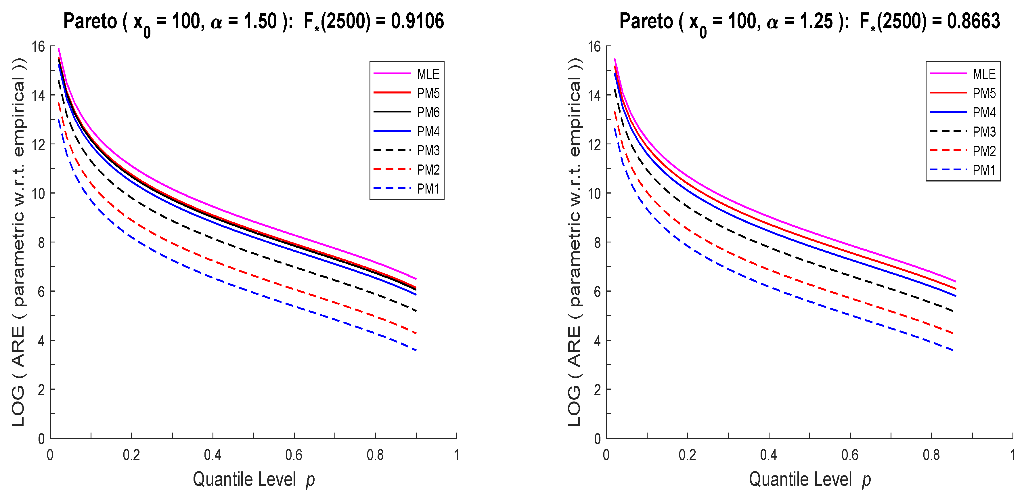
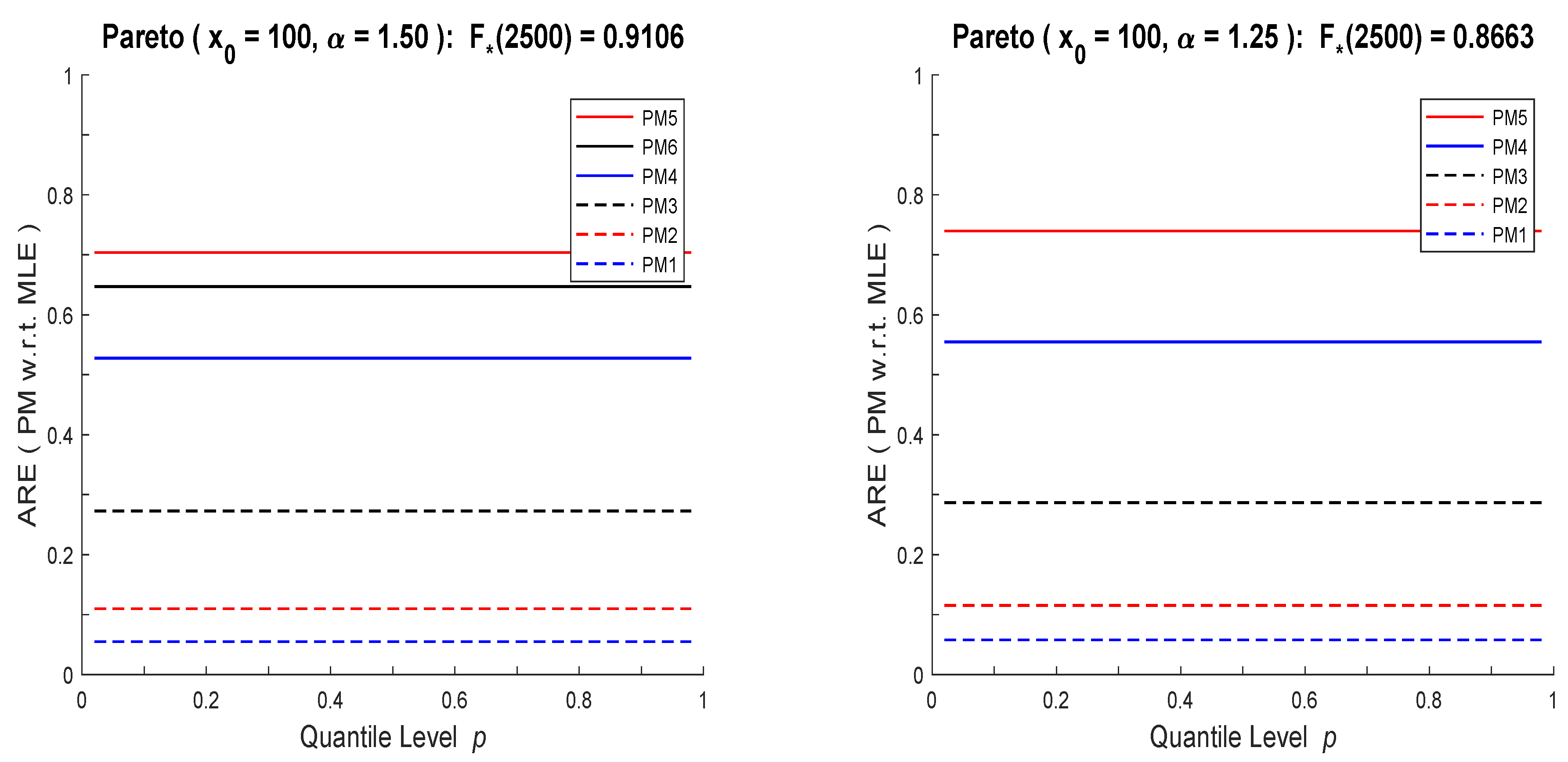
In Figure 2, RECs of quantile estimators of the Pareto ($x_0=100,\alpha$) distribution are plotted for the left-truncation level $t=500$ and right-censoring at $u=2500$. In the first column of plots, the distribution is heavy tailed ($\alpha =1.50$) with $F\left(t\right)=0.9106$, $F\left(u\right)=0.9920$, and $F_{*}\left(u\right|t;u)=0.9106$. In the second column of plots, the distribution has even heavier tail ($\alpha =1.25$) with $F\left(t\right)=0.8663$, $F\left(u\right)=0.9821$, and $F_{*}\left(u\right|t;u)=0.8663$. Due to the high bias of the empirical estimator (which goes to ∞ as $p\to 0$), the vertical axes are plotted on the logarithmic scale to minimize visual distortions. Comparison of plots shows the same ordering of PM curves as those under the exponential distribution assumption. The choice of $p_1\approx 0.80$ is also optimal for PM estimation. A change from heavy to even heavier tail and a decrease in the percentage of actually observed data $F_{*}\left(u\right|t;u)$ results in less pronounced shifts of the Pareto-based REC curves; but they are much higher than the exponential RECs. Thus, since both models are truncated and censored at the identical $t=500$ and $u=2500$, this suggests that the significant differences in the REC curves between the distributions can be used to construct a model selection method. This idea will be further discussed in Section 4.

4. Evaluation of Model Uncertainty

In this section, using simulated data we demonstrate how model uncertainty can emerge in a surprising way and examine how wrong quantile estimates can be when one makes incorrect modeling assumptions. In particular, we generate $n=50$ observations from the exponential distribution of Section 3.1 (with $x_0=100$, $\theta =500$, $t=500$, $u=2500$), fit the exponential model using MLE and PM ($p_1=0.80$) estimators to it, and perform standard model diagnostics (e.g., quantile-quantile plots) and validation (e.g., Kolmogorov-Smirnov and Anderson-Darling tests). As expected, the exponential distribution is not rejected by any of the tests. Then, using the same data we repeat the exercise by assuming a Pareto distribution, and find that it also passes all the tests. In both cases, we additionally compute AIC and BIC values, which under the incorrect Pareto assumption are better than the ones under the correct exponential assumption. Next, to make sure that this conclusion was not random, we simulate $n=50$ observations from the Pareto distribution of Section 3.2 (with $x_0=100$, $\alpha =1.50$, $t=500$, $u=2500$), fit and validate both models, and find yet again that both distributional assumptions are acceptable. This exercise shows that standard model diagnostic methods can mislead the decision maker, which would be not a major issue if quantile estimates based on incorrect modeling assumptions were close to the true values of quantiles, however, that’s not the case. For completeness, we include the empirical estimates of quantiles although it is known they are incorrect. Below we provide the details of the described exercises so the interested reader can reproduce the results.

The data sets were simulated using R with a seed of 200 (it is used to initialize the random number generator). They are presented in

Table 1. Left-truncated (at $t=500$) and right-censored (at $u=2500$) data simulated from the exponential ($x_0=100,\theta =500$) and Pareto ($x_0=100,\alpha =1.50$) distributions.

Exponential Data:	501, 501, 502, 502, 540, 551, 556, 556, 567, 599, 632, 642, 644, 646, 672, 675, 699, 711, 728, 745,
	750, 805, 829, 854, 869, 874, 889, 923, 961, 1012, 1034, 1046, 1054, 1102, 1107, 1169, 1178,
	1190, 1253, 1392, 1430, 1450, 1470, 1901, 1965, 2351, 2465, 2500, 2500, 2500.
Pareto Data:	516, 526, 535, 542, 550, 570, 593, 603, 605, 608, 609, 661, 674, 688, 694, 728, 734, 751, 751, 768,
	778, 782, 786, 797, 825, 836, 836, 847, 940, 962, 968, 1034, 1080, 1115, 1118, 1120, 1134, 1137,
	1175, 1213, 1224, 1271, 1379, 1725, 1861, 2000, 2500, 2500, 2500, 2500.

, where censored observations are italicized.

In Figure 3, the quantile-quantile plots (QQ-plots) are provided. The plots are parameter free. That is, since the exponential and Pareto distributions are location-scale and log-location-scale families, respectively, their QQ-plots can be constructed without first estimating model parameters. Note also that only actual data can be used in these plots (i.e., no observations $u=2500$). As is evident from Figure 3, the points in all graphs form a (roughly) straight line; thus both distributions are acceptable for both data sets.

To formally evaluate the appropriateness of the fitted model to data, we perform KS and AD goodness-of-fit tests. The models are fitted using two parameter estimation methods, MLE and PM ($p_1=0.80$), to check the sensitivity of overall conclusions to model fitting procedures. The values of the test statistics along with the corresponding p-values are reported in

Table 2. Parameter estimates, goodness-of-fit measures, and information criteria for the exponential and Pareto models fitted to the data sets of Table 1.

Assumed Model	Parameter Estimates	Goodness-of-Fit Measures		Information Criteria
		Kolmogorov-Smirnov	Anderson-Darling	AIC	BIC
		(p-Value *)	(p-Value *)
Exponential Data
Exponential	${\widehat{\theta }}_{\mathrm{MLE}}=595.57$	0.077 (0.914)	1.099 (0.317)	696.62	698.53
	${\widehat{\theta }}_{\mathrm{PM}}=554.23$	0.076 (0.637)	0.942 (0.374)	696.86	698.78
Pareto	${\widehat{\alpha }}_{\mathrm{MLE}}=1.491$	0.095 (0.371)	0.898 (0.344)	679.29	681.20
	${\widehat{\alpha }}_{\mathrm{PM}}=1.572$	0.109 (0.538)	1.112 (0.262)	682.92	684.83
Pareto Data
Exponential	${\widehat{\theta }}_{\mathrm{MLE}}=579.33$	0.109 (0.573)	0.564 (0.670)	695.99	697.90
	${\widehat{\theta }}_{\mathrm{PM}}=443.01$	0.102 (0.610)	1.006 (0.329)	696.12	698.03
Pareto	${\widehat{\alpha }}_{\mathrm{MLE}}=1.487$	0.128 (0.354)	1.025 (0.294)	678.29	680.20
	${\widehat{\alpha }}_{\mathrm{PM}}=1.816$	0.195 (0.000)	2.525 (0.000)	681.44	683.35

${}^{*}$ The p-values are computed using parametric bootstrap with 1000 simulation runs.

. (The p-values are computed using parametric bootstrap with 1000 simulation runs. For a brief description of the parametric bootstrap procedure, see, for example, Section 20.4.5 of Klugman et al. (2012)). We can see that except for one isolated case (Pareto data, Pareto model, PM estimation) the p-values are above 0.10 for both distributions, all parameter estimation methods, and both tests. Thus, the fitted exponential and Pareto models are acceptable for both data sets. In addition, the table contains AIC and BIC values, which can be used as model selection tools. Based on these metrics (smaller values are better), the Pareto model would be chosen for both data sets. Of course, the decision to accept Pareto when data came from an exponential distribution is incorrect.

Next, to see whether it really matters which model we select at this stage of the analysis, we have to examine the true probability models that generated data and check how much off target our upper quantile estimates are. For the data sets of Table 1, the underlying distributions are exponential ($x_0=100,\theta =500$) and Pareto ($x_0=100,\alpha =1.50$), with the quantile functions given by:

$$F^{-1}\left(p\right)=100-500log(1-p)\left(\mathrm{exponential}\right),F^{-1}\left(p\right)=100{(1-p)}^{-1/1.50}\left(\mathrm{Pareto}\right).$$

Thus, the true values of the 90%, 95% and 99% quantiles (estimation targets) are:

$$\mathrm{Exponential}:F^{-1}\left(0.90\right)=1251,F^{-1}\left(0.95\right)=1598,F^{-1}\left(0.99\right)=2403.$$

$$\mathrm{Pareto}:F^{-1}\left(0.90\right)=464,F^{-1}\left(0.95\right)=737,F^{-1}\left(0.99\right)=2154.$$

The quantile estimation results are summarized in

Table 3. Parametric and empirical estimates of the 90%, 95% and 99% quantiles for the exponential and Pareto data sets of Table 1.

Data Set	Estimation Methodology		Quantile Estimates
	Assumed Model	Estimator	${\widehat{\mathit{F}}}^{-1}\left(0.90\right)$	${\widehat{\mathit{F}}}^{-1}\left(0.95\right)$	${\widehat{\mathit{F}}}^{-1}\left(0.99\right)$
Exponential	Exponential	MLE	1471	1884	2843
		PM	1387	1774	2674
	Pareto	MLE	468	746	2194
		PM	436	679	1902
	Empirical	$---$	2004	2484	2500
Pareto	Exponential	MLE	1434	1836	2768
		PM	1123	1431	2146
	Pareto	MLE	471	750	2216
		PM	356	522	1269
	Empirical	$---$	1875	2500	2500

. There, we clearly see that the parametric estimates of the quantiles based on the correctly identified model are fairly close to their targets, but those based on the incorrect model are significantly off their targets. Also, the empirical estimates are way off target (${\widehat{F}}^{-1}\left(0.99\right)=2500$ for the exponential data set is a lucky coincidence, not a rule).

Finally, in

Table 4. Estimated Pareto and exponential RECs (MLE and empirical) at selected quantile levels. Model parameter estimates are from Table 2, based on the data of Table 1.

Quantile Level p	Exponential Data		Pareto Data
	Exponential Model	Pareto Model	Exponential Model	Pareto Model
0.05	8293	615,077	8792	611,390
0.10	1971	145,899	2089	145,025
0.25	267	19,631	283	19,513
0.50	47	3413	50	3393
0.75	13	877	14	872
0.90	6	344	6	342
0.95	4	228	5	227

we present estimated RECs, given by (11) and (17), at selected quantile levels. The curves are estimated using the MLE values from Table 2 and show how many times the parametric approach is more efficient than the empirical one in estimating a quantile. Note that as was seen in Figure 1 and Figure 2, RECs based on PM estimators have the same shapes as those of MLE, just rescaled by a constant (smaller than one). Thus PM based conclusions would not change from those of MLE and one method of analysis will be sufficient. What stands out from these computations is the vast differences between the corresponding exponential and Pareto RECs, when they are estimated using the same data set (especially for small p). We conjecture that with some additional work one can develop an effective diagnostic tool to differentiate between the models.

5. Concluding Remarks

The relative efficiency curves, REC, were introduced as a practical tool for comparison of two competing statistical procedures, when data are complete. In this paper, we have redesigned and extended such curves to the left-truncated and right-censored data scenarios that are common in insurance analytics. Our illustrations have focused on the parametric (MLE and PM) and empirical nonparametric approaches for estimation of quantiles that are key inputs for further risk analysis (e.g., contract pricing, risk measurement, capital allocation). Further, we have developed specific examples of RECs for exponential and single-parameter Pareto distributions under a few data truncation and censoring scenarios. Then, using simulated exponential and Pareto data we have examined how wrong quantile estimates can be when incorrect modeling assumptions are made. The numerical analysis involved application of standard model diagnostics and validation (e.g., QQ-plots, KS and AD tests, AIC and BIC criteria) and has demonstrated how those methods can mislead the decision maker. Finally, the newly developed RECs have been applied to study the discrepancies between the quality of quantile estimates of the fitted exponential and Pareto distributions. Our conclusion is that RECs have strong potential for being developed into an effective diagnostic tool in this context.

References

- Aggarwal, Ankur, Michael B. Beck, Matthew Cann, Tim Ford, Dan Georgescu, Nirav Morjaria, Andrew D. Smith, Yvonne Taylor, Andreas Tsanakas, Louise Witts, and et al. 2016. Model risk—Daring to open up the black box. British Actuarial Journal 21: 229–96. [Google Scholar] [CrossRef]
- Alexander, Carol, and Jose M. Sarabia. 2012. Quantile uncertainty and value-at-risk model risk. Risk Analysis 32: 1293–308. [Google Scholar] [CrossRef] [PubMed]
- Bignozzi, Valeria, Giovanni Puccetti, and Ludger Rüschendorf. 2015. Reducing model risk via positive and negative dependence assumptions. Insurance: Mathematics and Economics 61: 17–26. [Google Scholar] [CrossRef] [Green Version]
- Black, Rob, Andreas Tsanakas, Andrew D. Smith, Michael B. Beck, Iain D. Maclugash, Jasvir Grewal, Louise Witts, Nirav Morjaria, R. J. Green, and Zhixin Lim. 2018. Model risk: Illuminating the black box. British Actuarial Journal 23: 1–58. [Google Scholar] [CrossRef]
- Brazauskas, Vytaras, and Thomas Kaiser. 2004. Discussion of “Empirical estimation of risk measures and related quantities” by Jones and Zitikis. North American Actuarial Journal 8: 114–17. [Google Scholar] [CrossRef]
- Brazauskas, Vytaras, and Andreas Kleefeld. 2016. Modeling severity and measuring tail risk of Norwegian fire claims. North American Actuarial Journal 20: 1–16. [Google Scholar] [CrossRef]
- Brazauskas, Vytaras. 2009. Quantile estimation and the statistical relative efficiency curve. Metron LXVII: 289–301. [Google Scholar]
- Cairns, Andrew J. 2000. A discussion of parameter and model uncertainty in insurance. Insurance: Mathematics and Economics 27: 313–30. [Google Scholar] [CrossRef]
- Cambou, Mathieu, and Damir Filipović. 2017. Model uncertainty and scenario aggregation. Mathematical Finance 27: 534–67. [Google Scholar] [CrossRef]
- Cont, Rama, Romain Deguest, and Giacomo Scandolo. 2010. Robustness and sensitivity analysis of risk measurement procedures. Quantitative Finance 10: 593–606. [Google Scholar] [CrossRef] [Green Version]
- Embrechts, Paul, Bin Wang, and Ruodu Wang. 2015. Aggregation-robustness and model uncertainty of regulatory risk measures. Finance and Stochastics 19: 763–90. [Google Scholar] [CrossRef]
- Glasserman, Paul, and Xingbo Xu. 2014. Robust risk measurement and model risk. Quantitative Finance 14: 1–30. [Google Scholar] [CrossRef]
- Hartman, Brian, Robert Richardson, and Rylan Bateman. 2017. Parameter Uncertainty. Technical Report. Ottawa: Casualty Actuarial Society, Canadian Institute of Actuaries, Society of Actuaries. [Google Scholar]
- Hong, Liang, Todd Kuffner, and Ryan Martin. 2018. On prediction of future insurance claims when the model is uncertain. Variance 12: 90–99. [Google Scholar] [CrossRef]
- Jones, Bruce L., and Ricardas Zitikis. 2003. Empirical estimation of risk measures and related quantities (with discussion). North American Actuarial Journal 7: 44–54. Discussion: 8: 114–17; Reply: 8: 117–18. [Google Scholar] [CrossRef]
- Kaiser, Thomas, and Vytaras Brazauskas. 2006. Interval estimation of actuarial risk measures. North American Actuarial Journal 10: 249–68. [Google Scholar] [CrossRef]
- Klugman, Stuart A., Harry H. Panjer, and Gordon E. Willmot. 2012. Loss Models: From Data to Decisions, 4th ed. New York: Wiley. [Google Scholar]
- Modarres, Reza, Tapan K. Nayak, and Joseph L. Gastwirth. 2002. Estimation of upper quantiles under model and parameter uncertainty. Computational Statistics and Data Analysis 39: 529–54. [Google Scholar] [CrossRef]
- Samanthi, Ranadeera, Wei Wei, and Vytaras Brazauskas. 2017. Comparing the riskiness of dependent portfolios via nested L-statistics. Annals of Actuarial Science 11: 237–52. [Google Scholar] [CrossRef]
- Serfling, Robert J. 1980. Approximation Theorems of Mathematical Statistics. New York: Wiley. [Google Scholar]
- Yu, Daoping, and Vytaras Brazauskas. 2017. Model uncertainty in operational risk modeling due to data truncation: A single risk case. Risks 5: 49. [Google Scholar] [CrossRef]