Optimal Risk Budgeting under a Finite Investment Horizon

Abstract

The Growth-Optimal Portfolio (GOP) theory determines the path of bet sizes that maximize long-term wealth. This multi-horizon goal makes it more appealing among practitioners than myopic approaches, like Markowitz’s mean-variance or risk parity. The GOP literature typically considers risk-neutral investors with an infinite investment horizon. In this paper, we compute the optimal bet sizes in the more realistic setting of risk-averse investors with finite investment horizons. We find that, under this more realistic setting, the optimal bet sizes are considerably smaller than previously suggested by the GOP literature. We also develop quantitative methods for determining the risk-adjusted growth allocations (or risk budgeting) for a given finite investment horizon.

1. Introduction

The Growth-Optimal Portfolio (GOP) theory is influential in portfolio management Kelly (1956); Latane (1959); Markowitz (1959); Thorp and Kassouf (1967) along with modern portfolio theory Markowitz (1952). The GOP advocates to allocate investment capital at the (asymptotic) expected growth-optimal allocation so as to maximize the long-term expected compounded return of the portfolio. The attractive property of such portfolios includes optimal asymptotic growth, hence the name.

Despite its theoretical advantage, the growth-optimal allocation is also known to be generally too risky in practice Maclean et al. (2009); Thorp and Kassouf (1967); Vince (1990); Zenios and Ziemba (2006); Zhu (2007); Vince et al. (2013), and various methods have been suggested to reduce the risk exposure of expected growth-optimal allocations. One unsatisfactory aspect of these methods is that they are heuristic, and there is no theoretical justification on why and how to do it.

Recently, in Vince and Zhu (2015), Vince and Zhu observed that the GOP neglected two important practical considerations. First, the GOP optimizes the expected optimal growth assuming an infinite investment horizon. In reality, investors only invest in a finite time horizon. Second, in the GOP theory, the focus is on the expected growth only. Risk is ignored. In practice, of course, risk is a critical factor for any investment decision. Incorporating these two practical considerations in analyzing the bet size of the game of blackjack, Vince and Zhu showed in Vince and Zhu (2015) analytically and experimentally that the optimal bet size suggested by Kelly’s formula Kelly (1956), a predecessor of the GOP theory, needs to be adjusted downward considerably.

We consider our findings in terms of points within a return manifold, which we term a leverage space, the surface of expected geometric return in $N+1$ dimensions for N simultaneous events, at Q periods. Each of the N events is characterized by an axis in the $N+1$-dimensional manifold and bound between zero, where nothing is risked, and one, where the risk is as small as possible so as to assure total loss with the manifestation of the worst case. Further, whenever there exists a cumulative outcome or feedback mechanism that can range positive or negative from one discrete point to another, we reside at some loci on the return surface within the leverage space manifold whether we acknowledge this or not, and pay the consequences or reap the benefits of such loci therein.

GOP, in effect, states that one should select those coordinates in the leverage space at the (asymptotic, $Q\to \infty$) peak. We note that Kelly’s formula Kelly (1956) refers to this asymptotic peak. Using the model in Vince and Zhu (2013) to represent expected geometric return as a function of Q, we find that for a single position with a positive expectation, expected growth is always maximized at a fraction risked of 1.0 for $Q=1$. As Q increases, this expected growth-optimal fraction rapidly decreases toward its asymptotic value as specified by the Kelly criterion (the shape of the return surface within the leverage space manifold is a function of Q), and thus, we generally use this asymptotic value for all situations as a proxy for the actual expected growth-optimal fraction in all cases except for small values for Q. Given the unwieldy model for actual expected growth in Vince and Zhu (2013), we use as a proxy herein Kelly’s formula for the average expected growth per play assuming infinite play, express this as expected growth after Q plays, and very accurately derive values for the curve over the domain $f\in [0,1]$ at any given, but not too small values for Q in our analysis. The point becomes moot in the context discussed here as the important loci discussed in this paper do not appear until Q reaches satisfactory values to satisfy this requirement. Thus, the Kelly criterion solution is always less aggressive than what actually is the expected growth-optimal fraction for any finite horizon.

Further, as demonstrated in Vince and Zhu (2015), we scale the Kelly criterion answer using the worst case, so as to comport to being an actual fraction to risk so that multiple, simultaneous propositions can be considered properly (relative to each other), short sales considered, etc., such that we are always using a fraction and thus bounding the axes of the leverage space manifold at zero and one for all possible simultaneous propositions. This is discussed further at the beginning of Section 3.

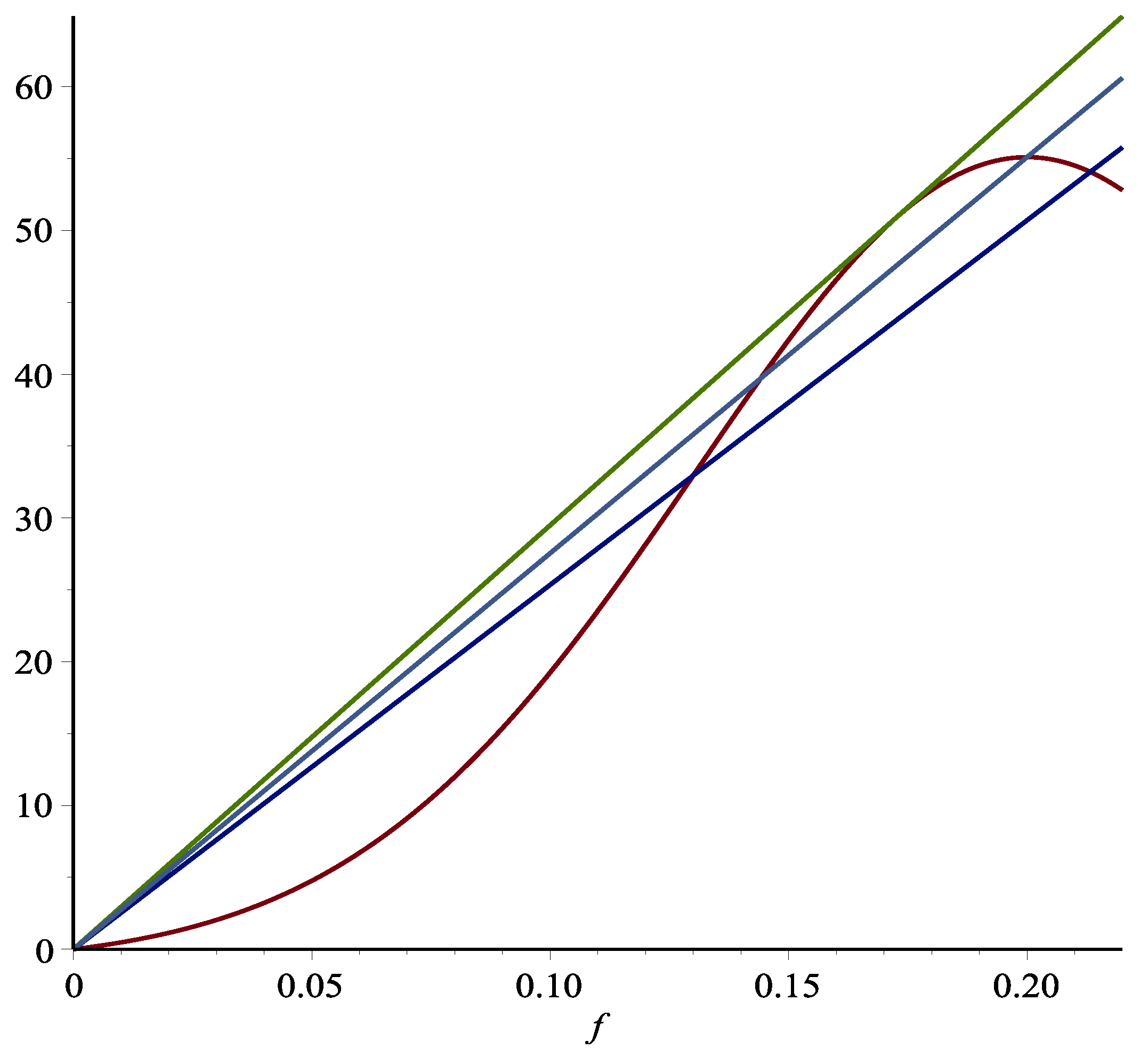
The results in Vince and Zhu (2015) were based on two simple observations: the graph of the total return function for playing blackjack hands a finite number of times is a bell-shaped curve, and the risk, as measured by the maximum drawdown, is approximately proportional to the bet size. As a result, the slope of the line connecting $(0,0)$ and any point on the return curve is proportional to the return/risk ratio where the risk is measured by the maximum drawdown. Thus, the optimal bet size maximizing the return/risk ratio is the line emanating from $(0,0)$ and tangent to the return curve depicted in Figure 1.

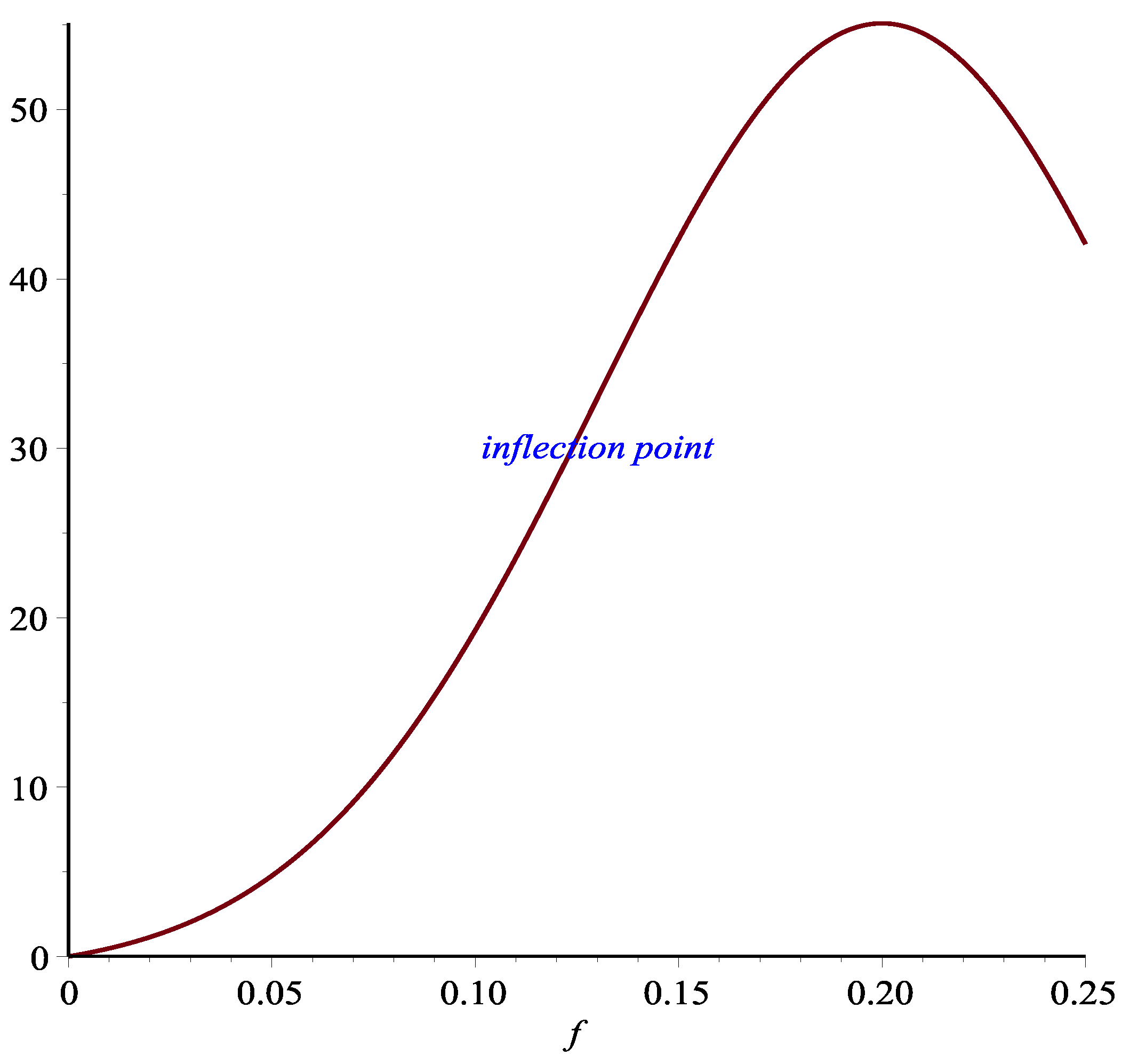
We can see that the corresponding bet size for this point is somewhat more conservative than the Kelly-optimal bet size corresponding to the peak of the return curve. Moreover, also noteworthy in Figure 1 is the inflection point corresponding to the lower line. This inflection point can be seen more clearly in Figure 2.

The inflection point is significant in that it is the boundary of increasing or decreasing marginal return when the bet size increases. If one were to pursue increasing the return/risk ratio, then it does not make sense to stop before reaching the inflection point. However, increasing the bet size beyond the inflection point arguably is a matter of choice. Because between the inflection point and the return/risk maximum point, while increasing the bet size still improves the return/risk ratio, the marginal benefit of doing so diminishes. Thus, the interval between the inflection point and the return/risk maximizing point is a reasonable region for players with different risk aversion to choose their appropriate strategy. Indeed, these observations are corroborated by Monte Carlo simulations in Vince and Zhu (2015).

Both of these aforementioned points are a function of horizon, Q, and migrate towards the asymptotic peak as $Q\to \infty$.1

Although Vince and Zhu (2015) focuses on bet size for playing blackjack, the idea and methods also apply to general capital allocation for investment problems involving multiple risky assets or investment strategies. In fact, inflection points have been discussed in Vince and Zhu (2013) in a more general context. The main goal of this paper is to provide a practical guide on how to implement the idea in Vince and Zhu (2013; 2015) for investment problems involving multiple investment instruments. When there are multiple assets involved, the path from the optimal GOP allocation to the completely riskless position of all cash (bonds) is not unique. In fact, there are infinitely many possible paths from which to choose. Although given a risk measure, one can argue it is reasonable to follow a path that on every level of the return manifold, the path should travel through the point that minimizes the risk measure. In reality, finding such a path may turn out to be very costly. Therefore, other alternative choices of paths should also be allowed. The risk measure when involving multiple assets and investment strategies is also more complicated. For each investment strategy, the same argument in Vince and Zhu (2015) still applies, and the size of the funds allocated to it is approximately proportional to the drawdown. However, the proportional constants for different investment strategies may well be different. Moreover, the total drawdown will also depend on how the drawdowns for different investment strategies are correlated, adding more technical issues into the equation.

Once a return/risk path is determined, the return function along this path becomes a one-variable function of the parameter that defines the path. One may attempt to use the method in Vince and Zhu (2015) to determine the trade-off between return and risk. However, the idea in Vince and Zhu (2015) as alluded to in the previous paragraph only works when the parameter is proportional to the risk. This only happens for a few return/risk paths. In practical capital allocation problems, the comparison of different return/risk paths is often necessary. We show that the inflection points on different return/risk paths are all on one manifold determined by Sylvester’s criterion of negative definiteness of a matrix involving the derivatives of the return functions and provides a reasonable approximation. Similarly, we also develop equations characterizing the manifolds of all return-/risk-optimal points.

The rest of the paper is arranged as follows: we first illustrate our results using a simple concrete example in the next section. Then, we discuss the general model and growth-optimal allocation in Section 3. Section 4 discusses the return/risk paths and special cases in which the methods in Vince and Zhu (2015) directly apply. In Section 5 and Section 6, we develop methods of characterizing the manifolds of inflection points and return-/risk-optimal points, respectively. We also discuss approximations where appropriate. We then discuss application examples in Section 7. We conclude in Section 8 and discuss avenues for further research regarding this material.

2. An Example

Let us consider playing a game where two coins are tossed independently at the same time. Coin 1 is a 0.50/0.50 coin that pays 2:1, and Coin 2 is a 0.60/0.40 coin that pays 1:1 (to be non-symmetrical, as the simplest case). We play $Q=50$ times. The joint probability distribution is summarized in

Table 1. Two coins.

Coin 1	Coin 2	Probability
2	1	0.3
2	−1	0.2
−1	1	0.3
−1	−1	0.2

.

For $f_1,f_2$ being the amounts risked on Coin 1 and Coin 2, respectively, $f_i\in [0,1],i=1,2$, then the expected return function is:

$$r(f_1,f_2)=\exp \left(50l(f_1,f_2)\right)-1,$$

where:

$$l(f_1,f_2)=[0.3ln(1+2f_1+f_2)+0.2ln(1+2f_1-f_2)+0.3ln(1-f_1+f_2)+0.2ln(1-f_1-f_2)]$$

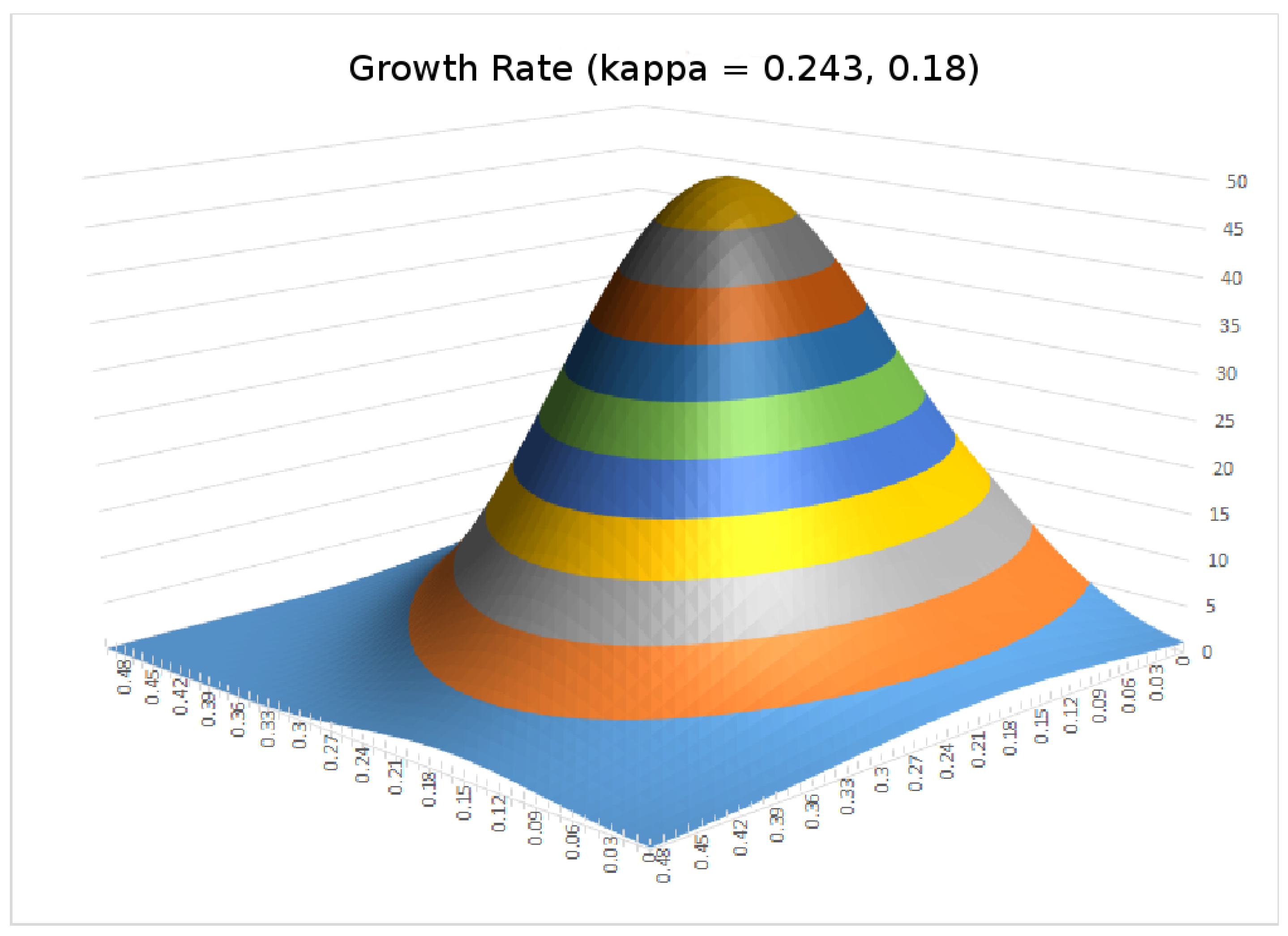
is the expected log return function. Figure 3 plots r as a function of $f_1$ and $f_2$.

Note that each of the four summands in the definition of $l(f_1,f_2)$ is a composition of the strictly concave log function and a nontrivial affine function and, therefore, strictly concave. Thus, $l(f_1,f_2)$ itself is also a strictly concave function on its domain in the leverage space $(f_1,f_2)\in [0,1)\times [0,1)$. We know that strictly concave functions have at most one maximum point. On the other hand, $l(f_1,f_2)$ approaches $-\infty$ as $(f_1,f_2)$ approaches the upper and right boundaries of the leverage space $[0,1)\times [0,1)$. Since both games have a positive expected return, neither the left boundary of the leverage space where $f_1=0$, nor the lower boundary where $f_2=0$ will contain the maximum for the log return function $l(f_1,f_2)$. Thus, $l(f_1,f_2)$ must attain a unique maximum in the interior of the leverage space. As the composition of the monotonic increasing function $exp\left(\right)$ and the log return functions $l(f_1,f_2)$, $r(f_1,f_2)$ and $l(f_1,f_2)$ share the same maxima, it follows that $r(f_1,f_2)$ also has a unique maximum in the interior of the leverage space, which is the Kelly-optimal bet sizes for these two games played simultaneously. We can determine this Kelly-optimal point by applying the first order necessary condition:

$$\begin{array}{c}\hfill \nabla r(f_1,f_2)=50\mathit{exp}\left(50l(f_1,f_2)\right)\nabla l(f_1,f_2)=0\end{array}$$

(1)

and represent it by the vector $\kappa =(0.243,0.180)$. As discussed above, $\kappa$ is the unique solution to (1).

As pointed out in Maier-Paape and Zhu (2018), practically important risk measures related to expected (log) drawdowns can be linearly approximated by position size. Thus, in what follows, we will use position size as a proxy for the risk, an approach already used in Vince and Zhu (2015). For a single game as discussed in Vince and Zhu (2015), the magnitude of this proportional constant is not important, as long as the expected (log) drawdown is approximately proportional to the bet size. Now that we are considering two different games together, the proportional constants for the two games are in general different. When trying to approximate the aggregated drawdown, it is now important to estimate the two different proportional constants. Simulating these two games for 2000 rounds of playing 50 simultaneous tosses ($Q=50$) each, then calculating the mean, demonstrates that for the two individual games, the expected drawdowns are proportional to $c_1{f}_1$ and $c_2{f}_2$, where $c_1=5.73$ and $c_2=6.12$, respectively.

Another complication in discussing the approximation of the aggregated drawdowns in this situation is that we need to consider the correlation of the two drawdowns. When the two drawdowns occur independently of each other (referring to the overlap of their duration in time), the aggregated drawdown is roughly the largest between the two linear approximations, i.e., $max(c_1{f}_1,c_2{f}_2)$. The other extreme is that the two drawdowns are completely dependent so that the aggregated drawdown is proportional to $c_1{f}_1+c_2{f}_2$. In general, there are some correlations between the drawdowns of the two games, and we get something in between.

For each level t of the return r, a risk-averse investor may select, on the level curve of $r(f_1,f_2)=t$, the point $(f_1\left(t\right),f_2\left(t\right))$ that minimizes the risk as measured by the drawdown. As t progresses from zero to the maximum of the return, $(f_1\left(t\right),f_2\left(t\right))$ will trace out a curve in the leverage space from $(0,0)$ to $\kappa$. Each different choice of the approximation of the drawdown corresponds to such a curve. If we draw all such curves, they then aggregately provide us a region in leverage space that represents allocations achieving minimum risk under the given return. Since it is impossible to trace infinitely many such curves, we focus on the two extreme cases alluded to above to derive the boundaries of this region.

Consider the completely dependent case first. Our problem becomes, for each $t\in [0,r(\kappa \left)\right]$,

$$\begin{array}{cc}\hfill \mathrm{minimize}& c_1{f}_1+c_2{f}_2\hfill \\ \hfill \mathrm{subject}\mathrm{to}& r(f_1,f_2)=t.\hfill \end{array}$$

(2)

Observing that changing $r(f_1,f_2)=t$ to $r(f_1,f_2)\ge t$ does not change the solution, we see that Problem (2) is a convex optimization problem and, therefore, has a unique solution determined by the Lagrange multiplier rule:

$$\nabla r=\lambda (c_1,c_2).$$

Taking the ratio of the two components and using the computation of $\nabla r$ in (1), we can see that the curve $(f_1\left(t\right),f_2\left(t\right))$ is determined by the equation:

$$\begin{array}{c}\hfill c_2\frac{\partial r}{\partial f_1}=c_1\frac{\partial r}{\partial f_2},\end{array}$$

(3)

starting from $\kappa$ until it intercepts one of the coordinate axes. Afterwards, it follows the intercepted coordinate axis to $(0,0)$. We will name this curve Path 1 for reference in the future.

The other extreme is that the two drawdowns always happen in non-overlapping time intervals. Then, we need to solve the convex constrained minimization problem:

$$\begin{array}{cc}\hfill \mathrm{minimize}& max(c_1{f}_1,c_2{f}_2)\hfill \\ \hfill \mathrm{subject}\mathrm{to}& r(f_1,f_2)\ge t.\hfill \end{array}$$

(4)

Here, the optimality condition is (see, e.g., Borwein and Zhu (2005)):

$$\nabla r=\lambda (\theta c_1,(1-\theta )c_2),\lambda >0,\theta \in [0,1].$$

In this optimality condition, $\theta =0$, corresponding to $c_2{f}_2>c_1{f}_1$, and leads to $f_2=0.18$. Similarly, $\theta =1$ corresponds to $c_2{f}_2<c_1{f}_1$ and leads to $f_1=0.243$. It follows that before either $f_1\left(t\right)$ reaches $0.243$ or $f_2\left(t\right)$ reaches $0.18$, we should always have $\theta \in (0,1)$, which corresponds to $c_2{f}_2=c_1{f}_1$. Thus, the path $(f_1\left(t\right),f_2\left(t\right))$ follows the line:

$$\begin{array}{c}\hfill c_2{f}_2=c_1{f}_1\end{array}$$

(5)

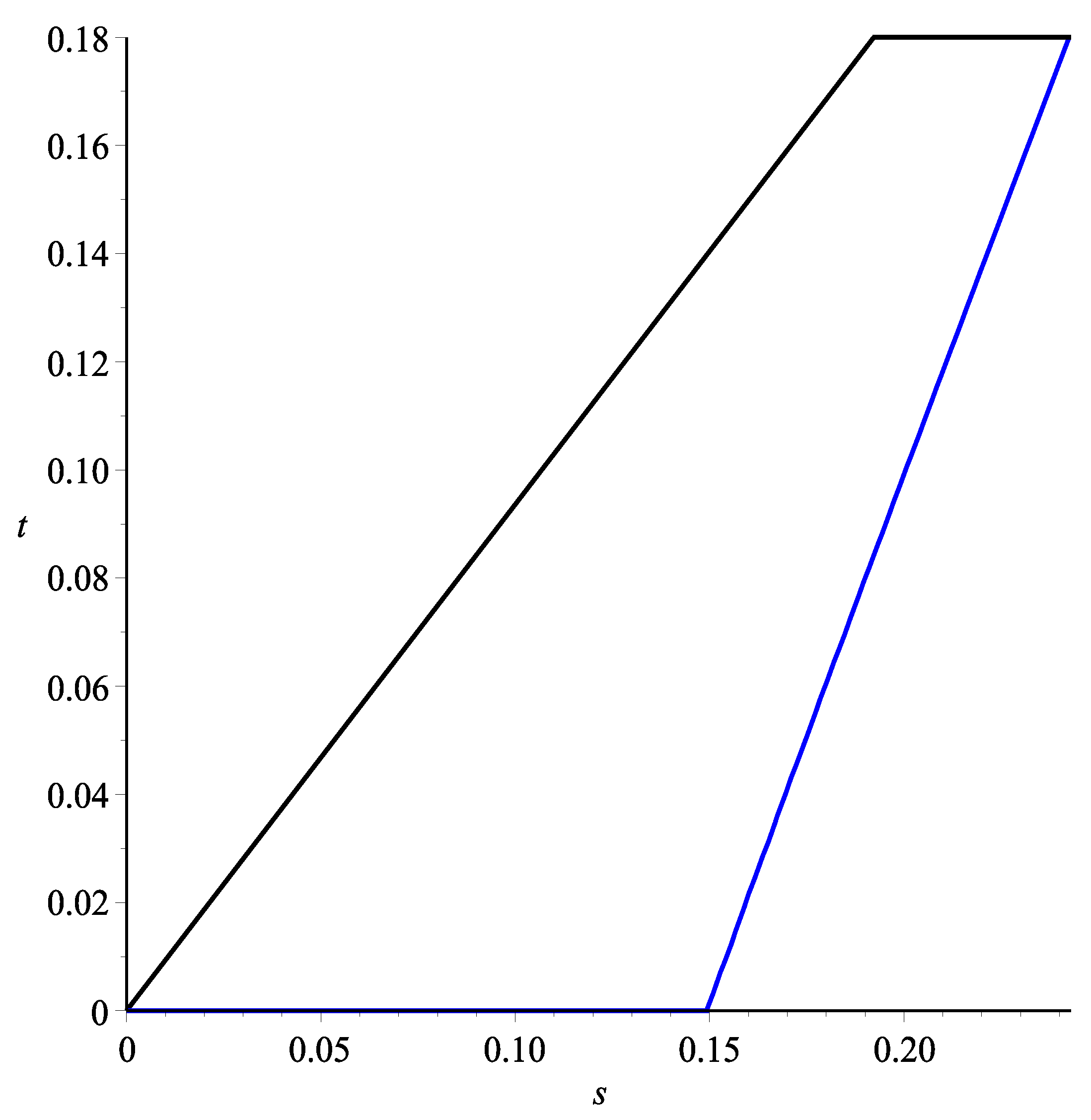
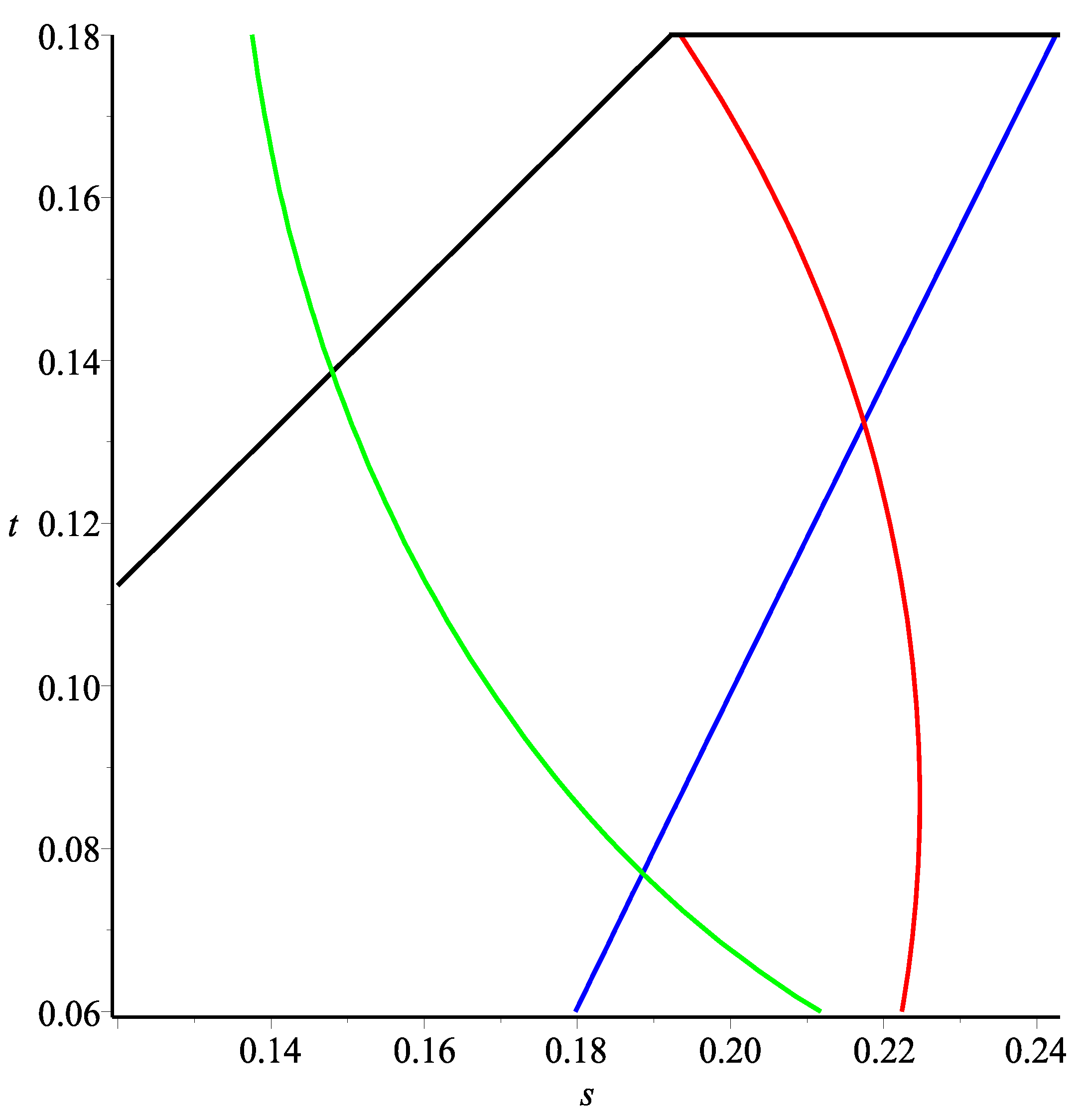
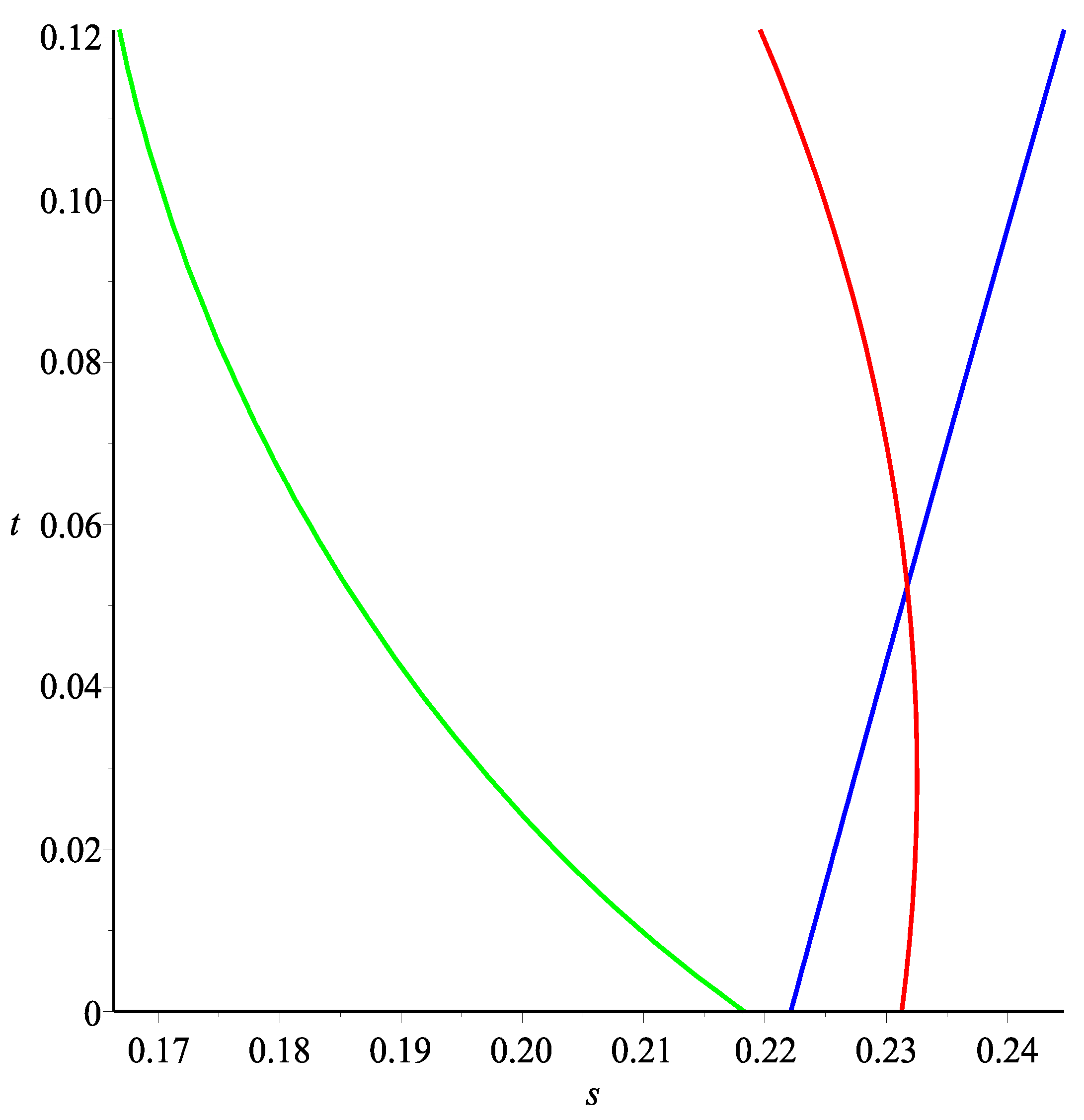
until either $f_1\left(t\right)$ reaches $0.243$ or $f_2\left(t\right)$ reaches $0.18$. After that, it follows the straight line to $\kappa =(0.243,0.18)$. We will name this curve Path 2. For $c_1=5.73$ and $c_2=6.12$, the two curves discussed above are illustrated in Figure 4, where the curves corresponding to (3) and (5) are colored in blue and black, respectively. In general, the drawdown will fall in between these two extreme cases.

Next, we consider the return/risk optimizing point $\zeta$ and the inflection point $\nu$ on these paths. As we will see in Section 5:

$$\begin{array}{c}\hfill min(-\frac{{\partial }^{2}r}{\partial f_1^2},\det (\mathrm{Hessian}\left(r\right)))=0\end{array}$$

(6)

determines the curve at which the inflection of the graph of r occurs. To determine $\zeta$ for the completely dependent case, we need to maximize $r(f_1,f_2)/(c_1{f}_1+c_2{f}_2)$. The optimality condition is:

$$0=\frac{\nabla r(f_1,f_2)(c_1{f}_1+c_2{f}_2)-r(f_1,f_2)(c_1,c_2)}{{(c_1{f}_1+c_2{f}_2)}^2}$$

which is equivalent to:

$$\nabla r(f_1,f_2)(c_1{f}_1+c_2{f}_2)=r(f_1,f_2)(c_1,c_2).$$

Using $(f_1,f_2)$ to dot product both sides and canceling $(c_1{f}_1+c_2{f}_2)$ yield:

$$\begin{array}{c}\hfill \nabla r(f_1,f_2)·(f_1,f_2)=r(f_1,f_2).\end{array}$$

(7)

It turns out that this is true in general (the proof uses a similar calculation involving subdifferentials for convex functions and will be given in Section 6). Thus, the $\zeta$ point corresponding to any curve will have to be on the curve defined by Equation (7). In particular, we can find the $\zeta$ points corresponding to the independent and completely dependent cases by looking at the interception of the corresponding curves as shown in Figure 5, in which the curves corresponding to Equations (6) and (7) are represented in red and green, respectively, and the blue and black curves again represent (3) and (5), respectively. The corresponding significant points are summarized in

Table 2. Two-coin example with $Q=50$.

	$\mathit{\nu }$	$\mathit{\zeta }$	$\mathit{\kappa }$
Path 1	(0.1885, 0.077)	(0.2175, 0.133)	(0.243, 0.18)
Path 2	(0.148, 0.1385)	(0.1935, 0.18)	(0.243, 0.18)

below.

3. The General Model

Consider investing in M investment systems represented by a random vector $X=(X_1,\dots ,X_M)$ with N different outcomes $\{b^1,\dots ,b^N\}$ where $b^n=(b_1^n,\dots ,b_M^n)$. The random variable $X_m$ represents the absolute gain (loss) of the $m^{\mathrm{th}}$ investment asset. We consider investing in those investment systems for Q holding periods and suppose that $Prob(X=b^n)=p_n$. We wish to determine how best to allocate funds into those investment systems. We re-scale so that the allocation can be represented in leverage space Vince (2009). Let $w_m=min\{b_m^1,\dots ,b_m^N\}$. Assume there is no arbitrage opportunities so that $w_m<0$ for all $m=1,\dots ,M$. Define the scaled random vector $Y=(-X_1/w_1,\dots ,-X_M/w_M)$ and the scaled outcome $a^n=(-b_1^n/w_1,\dots ,-b_M^n/w_M)$. Then, $Prob(Y=a^n)=p_n$. Now, each allocation can be represented by a vector $f=(f_1,\dots ,f_M)\in {[0,1]}^M$ where $f_m$ represents the fraction of the total number of shares one can invest in the $m^{\mathrm{th}}$ investment vehicle such that the worst loss $w_m$ will result in the loss of all the investment capital. We further assume that the M investment assets are independent enough so that:

$$\begin{array}{c}\hfill \mathrm{rank}[a^1,a^2,\dots ,a^N]=M.\end{array}$$

(8)

We note that condition (8) amounts to saying that there does not exist a nontrivial portfolio x such that $x·a^n=0$ for all $n=1,2,\dots ,N$. Since in this paper, we consider the simplified case where the riskless bond has an interest of zero, such a portfolio, in fact, replicates a riskless bond. In other words, we are considering a market in which there is no nontrivial bond replicating portfolio as defined in Maier-Paape and Zhu (2018).

Given the above setting, the expected gain per period is:

$$G_X\left(f\right):={\Pi }_{n=1}^N{(1+f·a_n)}^{p_n}.$$

Then, the total return can be approximated by $r_Q\left(f\right)={\left[G_X\left(f\right)\right]}^Q-1$. We have seen in Vince and Zhu (2015) that, for reasonably large Q, this approximation is quite accurate for the case of $M=1$. Thus, we will use this approximation in the analysis below. We note that using the log return function:

$$\begin{array}{c}\hfill l_X\left(f\right):=\sum _{n=1}^N{p}_{n}ln(1+f·a_n)\end{array}$$

(9)

we have the representation:

$${\left[G_X\left(f\right)\right]}^Q=\exp \left(Q{l}_X\left(f\right)\right).$$

Since the exponential function is monotone increasing and the log return function is strictly concave given Condition (8) (see (Maier-Paape and Zhu 2018, Proposition 6)), $r_Q\left(f\right)$ attains a unique maximum, which can be determined by solving the equation:

$$0=\nabla r_Q\left(f\right)=Q\exp \left(Q{l}_X\left(f\right)\right)\nabla l_X\left(f\right),$$

or equivalently:

$$\nabla l_X\left(f\right)=0.$$

We denote the solution $\kappa$ and note that this is the asymptotic growth-optimal allocation and therefore is independent of Q.

4. Return/Risk Paths

As illustrated in the example discussed in Section 2, we know that the allocation $\kappa$ is usually too risky. In practice, one needs to reduce the risk and take a middle ground between $f=\overrightarrow{0}$ and $f=\kappa$. It is clear from the example in Section 2 that there are many possible paths connecting these two possible allocations providing various trade-offs between risk and return.

Definition 1.

Let X be the vector of random variables introduced in Section 3 representing the gains of a group of risky assets. A mapping $f:[a,b]\to R^M$ is called a return/risk path with respect to X, if it has the following properties

1. 

f has piecewise continuous second order derivatives.

2. 

$f\left(a\right)=0$ and $f\left(b\right)=\kappa$.

3. 

$t\mapsto l_X\left(f\left(t\right)\right)$ is an increasing function on $[a,b]$.

4. 

There is a risk measure m on the leverage space such that $t\mapsto m\left(f\right(t\left)\right)$ is an increasing function on $[a,b]$.

5. 

$\nabla l_X\left(f\left(t\right)\right)f^{\prime \prime }\left(t\right)=0$ for all $t\in [a,b]$ where $f^{\prime \prime }\left(t\right)$ exists.

The meaning of Properties 4 and 5 is that the return/risk path must move toward the direction of increasing the reward with the maximum rate while increasing the risk. It is easy to see that both Path 1 and Path 2 in the example in Section 2 are return/risk paths. Along such paths, we can show that an inflection point always exits as long as Q is large enough.

Theorem 1.

Let $f:[a,b]\to R^M$ be a return/risk path. Then, when Q is sufficiently large, the function $t\mapsto r_Q\left(f\left(t\right)\right)$ has an inflection point on $(a,b)$, which is determined by the equation:

$$\begin{array}{c}\hfill Q{[\nabla l_X\left(f\left(t\right)\right)·f^{\prime }\left(t\right)]}^2+\langle f^{\prime }\left(t\right),\mathrm{Hessian}{l}_X\left(f\left(t\right)\right)f^{\prime }\left(t\right)\rangle =0.\end{array}$$

(10)

Proof. 

Direct computation shows that:

$$\frac{\partial r_Q\left(f\left(t\right)\right)}{\partial t}=Q\exp \left(Q{l}_X\left(f\left(t\right)\right)\right)[\nabla l_X\left(f\left(t\right)\right)·f^{\prime }\left(t\right)]$$

and:

$$\frac{{\partial }^2{r}_Q\left(f\left(t\right)\right)}{\partial t^2}=Q\exp \left(Q{l}_X\left(f\left(t\right)\right)\right){\varphi }_Q\left(t\right),$$

where:

$${\varphi }_Q\left(t\right):=Q{[\nabla l_X\left(f\left(t\right)\right)·f^{\prime }\left(t\right)]}^2+\langle f^{\prime }\left(t\right),\mathrm{Hessian}{l}_X\left(f\left(t\right)\right)f^{\prime }\left(t\right)\rangle .$$

Since there are only finitely many points on $[a,b]$ where $f^{\prime \prime }\left(t\right)$ does not exist, we denote $b^{\prime }$ as the last such point before b. Since $\kappa$ is unique, $l_X\left(f\left(b\right)\right)>l_X\left(f\left(b^{\prime }\right)\right)$. Thus, there are infinitely many $t\in [b^{\prime },b]$ where $\nabla l_X\left(f\left(t\right)\right)·f^{\prime }\left(t\right)>0$. Thus, we can choose $c\in (b^{\prime },b)$ such that $\nabla l_X\left(f\left(c\right)\right)·f^{\prime }\left(c\right)>0$. Observing that $\nabla l_X\left(f\left(b\right)\right)=\nabla l_X\left(\kappa \right)=0$ and $\mathrm{Hessian}{l}_X\left(\kappa \right)$ is negative definite, we have ${\varphi }_Q\left(b\right)=\langle f^{\prime }\left(b\right),\mathrm{Hessian}{l}_X\left(\kappa \right)f^{\prime }\left(b\right)\rangle <0$. On the other hand, for Q sufficiently large:

$$\begin{array}{c}\hfill {\varphi }_Q\left(c\right):=Q{[\nabla l_X\left(f\left(c\right)\right)·f^{\prime }\left(c\right)]}^2+\langle f^{\prime }\left(c\right),\mathrm{Hessian}{l}_X\left(f\left(c\right)\right)f^{\prime }\left(c\right)\rangle >0.\end{array}$$

(11)

Thus, ${\varphi }_Q\left(t\right)=0$ has a solution on $(c,b)$. □

Since c can be chosen arbitrarily close to b, when $Q\to \infty$, the inflection point ${\nu }_Q$ related to Q approaches $\kappa$.

On the other hand, the relationship between the risk measure and the parameters in these two paths is different. For Path 2, the risk measure is piecewise linearly related to the parameter t. Thus, we can use t as a proxy for the risk and using the method in Vince and Zhu (2015) for one risky asset to determine t values corresponding to the inflection point and the return/risk maximum point. However, this is not the case for Path 1 in which the risk $c_1{f}_1\left(t\right)+c_2{f}_2\left(t\right)$ as a nonlinear function of t is not proportional to t. Thus, it is not always possible to use the return/risk path to convert a problem involving multiple strategies into one with only one parameter and use the method discussed in Vince and Zhu (2015). In the following two sections, we seek more generic ways of finding inflection points and return/risk maximizing points.

5. Determining the Manifold of Inflection Points Using Sylvester’s Criterion

Next, we show that, similar to the example discussed in Section 2, in general, the function $r_Q\left(f\right)$ is concave near $\kappa$.

Theorem 2.

(Concavity) The function $r_Q\left(f\right)$ is concave near κ.

Proof. 

Recall that the concavity of a multi-variable function at a given point is characterized by its Hessian to be negative definite. Calculating the mixed second order partial derivative of $r_Q\left(f\right)$, we have:

$$\frac{{\partial }^2}{\partial f_i\partial f_j}{r}_Q\left(f\right)=Q\exp \left(Q{l}_X\left(f\right)\right)\left(\frac{{\partial }^2}{\partial f_i\partial f_j}{l}_X\left(f\right)+Q\frac{\partial l_X\left(f\right)}{\partial f_i}\frac{\partial l_X\left(f\right)}{\partial f_j}\right).$$

Since, for $i=1,\dots ,N$,

$$\frac{\partial l_X\left(\kappa \right)}{\partial f_i}=0$$

We have:

$$\frac{{\partial }^2}{\partial f_i\partial f_j}{r}_Q\left(\kappa \right)=Q\exp \left(Q{l}_X\left(\kappa \right)\right)\frac{{\partial }^2{l}_X\left(\kappa \right)}{\partial f_i\partial f_j}.$$

It follows that:

$$\mathrm{Hessian}\left(r_Q\left(\kappa \right)\right)=Q\exp \left(Q{l}_X\left(\kappa \right)\right)\mathrm{Hessian}\left(l_X\left(\kappa \right)\right).$$

The concavity of $l_X\left(f\right)$ implies that $\mathrm{Hessian}\left(r_Q\left(\kappa \right)\right)$ is negative definite. Since the second order partial derivatives of $r_Q\left(f\right)$ are continuous around $\kappa$, the Hessian of $r_Q\left(\kappa \right)$ is negative definite in the neighborhood of $\kappa$. Thus, $r_Q\left(f\right)$ is concave near $\kappa$. □

It is clear that the inflection point occurs where the concavity of $r_Q\left(f\right)$ changes. A characterization of this set is the following:

Theorem 3.

(Set of inflection points) The inflection point along any risk return path is contained in the following set of f in leverage space characterized by:

$$\begin{array}{c}\hfill min\left(-a_{11}\left(f\right),\det \left[\begin{array}{cc}{a}_{11}\left(f\right)& a_{12}\left(f\right)\\ a_{21}\left(f\right)& a_{22}\left(f\right)\end{array}\right],\dots ,{(-1)}^N\det \left[\begin{array}{cccc}{a}_{11}\left(f\right)& a_{12}\left(f\right)& \dots & a_{1N}\left(f\right)\\ a_{21}\left(f\right)& a_{22}\left(f\right)& \dots & a_{2N}\left(f\right)\\ \dots & \dots & \dots & \dots \\ a_{N1}\left(f\right)& a_{N2}\left(f\right)& \dots & a_{NN}\left(f\right)\end{array}\right]\right)=0.\end{array}$$

where $a_{ij}\left(f\right):=\frac{{\partial }^2}{\partial f_i\partial f_j}{l}_X\left(f\right)+Q\frac{\partial l_X\left(f\right)}{\partial f_i}\frac{\partial l_X\left(f\right)}{\partial f_j}$.

Proof. 

Sylvester’s criterion for the negative definiteness of a matrix tells us that $r_Q\left(f\right)$ is negative definite if and only if:

$$\begin{array}{c}\hfill -a_{11}\left(f\right)>0,\det \left[\begin{array}{cc}{a}_{11}\left(f\right)& a_{12}\left(f\right)\\ a_{21}\left(f\right)& a_{22}\left(f\right)\end{array}\right]>0,\dots ,{(-1)}^N\det \left[\begin{array}{cccc}{a}_{11}\left(f\right)& a_{12}\left(f\right)& \dots & a_{1N}\left(f\right)\\ a_{21}\left(f\right)& a_{22}\left(f\right)& \dots & a_{2N}\left(f\right)\\ \dots & \dots & \dots & \dots \\ a_{N1}\left(f\right)& a_{N2}\left(f\right)& \dots & a_{NN}\left(f\right)\end{array}\right]>0.\end{array}$$

Thus, the set in the theorem characterizes the boundary where this condition is violated for the first time: the potential inflection points. □

We note that the computation in determining the set given in Theorem 3 is quite involved. A practical (conservative) approximation is:

$$\begin{array}{c}\hfill \left\{f\in R^N:min\left(-a_{11}\left(f\right),-a_{22}\left(f\right),\dots ,-a_{NN}\left(f\right)\right)=0\right\}.\end{array}$$

(12)

6. Determining the Manifold of Return/Risk Maximum Points

We now turn to the manifolds of return/risk maximum points. We begin by a general definition of a kind of risk measure that covers the several patterns of risks discussed in Section 2 using the idea in Artzner et al. (1999).

Definition 2.

We say $m:R^M\to R$ is a risk measure coherent with the investment allocation f if m is convex $m\left(0\right)=0$ and $m\left(tf\right)=tm\left(f\right)$ for any $t>0$.

Coherent risk measures have the following serendipitous property:

Lemma 1.

Let $m\left(f\right)$ be a risk measure coherent with the investment allocation f. Then, for any $\xi \in \partial m\left(f\right)$, the convex subdifferential of m at f, we have:

$$m\left(f\right)=\langle \xi ,f\rangle .$$

Proof. 

The definition of the convex subdifferential $\xi \in \partial m\left(f\right)$ implies that:

$$m\left(z\right)-m\left(f\right)\ge \langle \xi ,z-f\rangle ,\forall z.$$

For $t>0$, setting $z=tf$ in the above inequality and using the coherent property of $m\left(f\right)$ yield:

$$(t-1)m\left(f\right)\ge (t-1)\langle \xi ,f\rangle ,\forall t>0.$$

Hence:

$$m\left(f\right)=\langle \xi ,f\rangle .$$

Now, we can characterize the manifold in leverage space that maximizes the return/risk ratio.

Theorem 4.

Let $m\left(f\right)$ be a risk measure coherent to the investment allocation f. Then, the set of allocations f that maximizes the return/risk ratio $r_Q\left(f\right)/m\left(f\right)$ is contained in the set:

$$\{f:\langle \nabla r_Q\left(f\right),f\rangle =r_Q\left(f\right)\}.$$

Proof. 

We observe that maximizing $r_Q\left(f\right)/m\left(f\right)$ is equivalent to the problem:

$$\begin{array}{cc}\hfill \mathrm{maximize}& \frac{r_Q\left(f\right)}{y}\hfill \\ \hfill \mathrm{subject}\mathrm{to}& m\left(f\right)-y\le 0,\hfill \end{array}$$

(13)

and the maximum is always attained when $y=m\left(f\right)$. The solution to the above problem belongs to:

$$\left(\frac{\nabla r_Q\left(f\right)}{y},-\frac{r_Q\left(f\right)}{y^2}\right)\in \lambda (\partial m\left(f\right),-1),$$

or:

$$\begin{array}{c}\hfill \nabla r_Q\left(f\right)\in \lambda y\partial m\left(f\right)\end{array}$$

(14)

and:

$$\begin{array}{c}\hfill r_Q\left(f\right)=\lambda y^2,\end{array}$$

(15)

where $\lambda$ is the Lagrange multiplier. Using Lemma 1 and inclusion (14), we have:

$$\langle \nabla r_Q\left(f\right),f\rangle =\lambda ym\left(f\right).$$

Combining this with (15) and $y=m\left(f\right)$, we arrive at:

$$\langle \nabla r_Q\left(f\right),f\rangle =r_Q\left(f\right).$$

Note that the linear approximation of drawdown is coherent with the investment allocation f. Many other types of risk measures also have this coherent property. □

7. Applications

We now turn to concrete examples to illustrate how to apply the theory discussed in the previous sections.

Example 1.

First, we recall the example of betting two simultaneous hands of blackjack in Vince and Zhu (2015). In this example, although there are two players involved, their strategy is the same. Thus, by symmetry, we can reason that the two players should use the same bet size. As a result, the problem is reduced such that there is only one bet size to calculate, and it can be solved using the methods in Vince and Zhu (2015).

However, in general, such a reduction is most of the time impossible.

Example 2.

A small, private equity firm is considering further funding for two very separate companies over the course of 72 months (six years) into the future. They wish to maximize their marginal increase in return with respect to the marginal increase in risk over this period, investing simultaneously in both companies.

Their study of these companies reveals that for each million provided in funding, Company A will show a monthly profit of $15,300 with a probability of 0.4 or a loss of $5000 with a probability of 0.6.

In considering Company B, there is a 0.8 probability of a $5000 monthly profit and a 0.2 probability of a $9200 monthly loss.

Assuming the returns on the two companies are statistically independent leads to the joint probabilities represented in

Table 3. Two companies.

Company A	Company B	Probability
−5000	−9200	0.12
−5000	5000	0.48
15,300	−9200	0.068
15,300	5000	0.32

.

However, further analysis of the past, given that the month-by-month performance of the two companies is in part contingent on business conditions, amends the probabilities to show greater interdependency, and our private equity firm deems the probabilities associated with these outcomes, when taken together, to be more accurately as in

Table 4. Two companies adapted.

Company A	Company B	Probability
−5000	−9200	0.2
−5000	5000	0.36
15,300	−9200	0.06
15,300	5000	0.38

.

Thus, the log return function and the cumulative return function in this case are:

$$l(f_1,f_2)=0.2ln(1-f_1-f_2)+0.36ln(1-f_1+\frac{5,000}{9,200}{f}_2)+0.06ln(1+\frac{15,300}{5,000}{f}_1-f_2)+0.38ln(1+\frac{15,300}{5,000}{f}_1+\frac{5,000}{9,200}{f}_2)$$

and:

$$r(f_1,f_2)=exp\left(72l(f_1,f_2)\right)-1,$$

respectively.

Numerically solving equation:

$$\nabla r(f_1,f_2)=0,$$

we find the peak of the (asymptotic) expected growth-optimal allocations to be $\kappa =(0.245,0.121)$ for Company A and Company B, respectively, with an average growth per month of $1.0981493$. Next, we consider the risk-adjusted return. In this case, since we only invest in a relatively short 72-month time-frame, it is reasonable to assume the risk related to the two companies is proportional to the largest monthly loss of −5000 and −9200, respectively. In the leverage space, this is to say the risks of Companies A and B are proportional to $f_1$ and $f_2$, respectively. Moreover, the probability of such losses occurring simultaneously is relatively high at $20\%$. Therefore, we assume that the aggregated risk is proportional to their sum $f_1+f_2$. We can see that the path that corresponds to the least risk for each level set is given by the equation:

$$\frac{\partial r}{\partial f_1}=\frac{\partial r}{\partial f_2}.$$

This path is depicted in Figure 6, which follows the horizontal axis and then the blue line. Depicted in Figure 6 as well are the curves corresponding to the inflection points in green and the return/risk maximizing points in red, calculated using the methods in Section 5 and Section 6. This gives us an estimate of ${\nu }_{72}=(0.218,0)$ and ${\zeta }_{72}=(0.23,0.05)$.

8. Conclusions and Further Research

Theoretical analysis, Monte Carlo simulation, and analysis of real-world examples showed that by the practical consideration of investment in a finite horizon and adjusting for risk, the leverage on different risky investment strategies suggested by the classical growth-optimal portfolio theory needs to be adjusted down considerably. We show that the inflection point and return/risk maximizing point discussed in Vince and Zhu (2015) are reasonable loci in leverage space in cases of capital allocation to risky assets or investment strategies. However, when multiple strategies are involved, reducing risk exposure from the growth optimal allocation, $\kappa$, there exists infinitely many choices of paths. Analyzing the problem path by path is difficult. We established equations for determining the manifolds of inflection points and the return/risk maximizing points. These equations can be solved numerically to determine a region for reasonable choices of leverage. Examples were presented to show how to apply these methods in practice.

As usual, our research here leads to additional questions of practical importance. For example, portfolio insurance allocates a certain percentage to the underlying asset or portfolio based on the delta of a hypothetical option on the underlying asset or portfolio. Thus, portfolio insurance is a practice where one traverses along the return curve between its bounds as a function of the underlying price relative to its hypothetical option. The curve is identical in shape to the return curves discussed here, as reinvestment is constantly occurring (and thus, delta and f are interchangeable in this context), yet, the practitioners, in order to mimic the hypothetical option, are not capitalizing on any of the important growth-regulation points mentioned in this paper.

Similarly, inverse Exchange Traded Funds (ETFs) and leveraged ETFs (cases of constant reinvestment) have a delta embedded within them as:

$$delta=\frac{ETFprice·leveragefactor·(long=1,short=-1)}{UnderlyingPrice}.$$

This delta too, a number between zero and some number whose absolute value can be greater than one, is followed so as to track the promoted criterion of the ETF, e.g., “triple long ETF”. Yet, as with portfolio insurance, the implementors, in keeping with the promoted criterion of the ETF, are not able to capitalize on the important growth-regulating points (perhaps to be used as bounds on the delta). Further research into this area is clearly warranted.

References

- Artzner, Philippe, Freddy Delbaen, Jean-Marc Eber, and David Heath. 1999. Coherent measures of risk. Mathematical Finance 9: 203–28. [Google Scholar] [CrossRef]
- Borwein, Jonathan M., and Qiji Zhu. 2005. Techniques of Variational Analysis. New York: Springer. [Google Scholar]
- Kelly, John L., Jr. 1956. A new interpretation of information rate. Bell System Technical Journal 35: 917–26. [Google Scholar] [CrossRef]
- Latane, Henry Allen. 1959. Criteria for choice among risky ventures. Journal Political Economy 52: 75–81. [Google Scholar] [CrossRef]
- Maier-Paape, Stanislaus, and Qiji Zhu. 2018. A general framework for portfolio theory. Part I: Theory and examples. Risks 6: 53. [Google Scholar] [CrossRef]
- Maier-Paape, Stanislaus, and Qiji Zhu. 2018. A general framework for portfolio theory. Part II: Drawdown measures. Risks 6: 76. [Google Scholar] [CrossRef]
- MacLean, Leonard C., Edward O. Thorp, and William T. Ziemba, eds. 2009. The Kelly Capital Growth Criterion: Theory and Practice. Singapore: World Scientific. [Google Scholar]
- Markowitz, Harry. 1952. Portfolio selection. Journal of Finanace 7: 77–91. [Google Scholar]
- Markowitz, Harry. 1959. Portfolio Selection. Cowles Monograph. New York: Wiley, vol. 16. [Google Scholar]
- Thorp, Edward O., and Sheen T. Kassouf. 1967. Beat the Market. New York: Random House. [Google Scholar]
- Vince, Ralph. 1990. Portfolio Management Formulas. New York: John Wiley and Sons. [Google Scholar]
- Vince, Ralph. 2009. The Leverage Space Trading Model. Hoboken: John Wiley and Sons. [Google Scholar]
- Vince, Ralph, and Qiji Jim Zhu. 2013. Inflection point significance for the investment size. SSRN 17. [Google Scholar] [CrossRef]
- Vince, Ralph, and Qiji Jim Zhu. 2015. Optimal betting sizes for the game of blackjack. Risk Journals Portfolio Management 4: 53–75. [Google Scholar] [CrossRef]
- Zenios, Stavros A., and William T. Ziemba, eds. 2006. The Kelly criterion: Theory and practice. In Handbook of Asset and Liability Management Volume A: Theory and Methodology. North Holland: Elsevier. [Google Scholar]
- Zhu, Qiji Jim. 2006. Mathematical analysis of investment systems. Journal of Mathematical Analysis and Applications 326: 708–20. [Google Scholar] [CrossRef]
- Zhu, Qiji Jim, Ralph Vince, and Steven Malinsky. 2013. A dynamic implementations of the leverage space portfolio. SSRN. [Google Scholar] [CrossRef]