Abstract
In this paper, we study a generalised CIR process with externally-exciting and self-exciting jumps, and focus on the distributional properties and applications of this process and its aggregated process. The aim of the paper is to introduce a more general process that includes many models in the literature with self-exciting and external-exciting jumps. The first and second moments of this jump-diffusion process are used to calculate the insurance premium based on mean-variance principle. The Laplace transform of aggregated process is derived, and this leads to an application for pricing default-free bonds which could capture the impacts of both exogenous and endogenous shocks. Illustrative numerical examples and comparisons with other models are also provided.
Keywords:
contagion risk; insurance premium; aggregate claims; default-free bond pricing; self-exciting process; hawkes process; CIR process JEL Classification:
G22; G13; C02
1. Introduction
Over recent years, self-exciting processes, especially the Hawkes point processes, have been brought to bear in the modelling and analysis of phenomena as diverse as earthquakes, credit defaults and arrivals of orders in the limit-order books in financial markets. Numerous papers have looked at modelling finance and insurance risk based on them. The theoretical foundation can be traced back to a series of papers written by Hawkes (1971a, 1971b); Hawkes and Oakes (1974); Brémaud and Massoulié (1996, 2001, 2002); and more recently, Dassios and Zhao (2011); Zhu (2013a, 2015); Jaisson and Rosenbaum (2015) and Boumezoued (2016). Early applications concentrated on the fields such as seismology (see Vere-Jones (1975, 1978); Adamopoulos (1976); Ozaki (1979); Vere-Jones and Ozaki (1982) and Ogata (1988)).
Recently, rapidly growing applications have emerged in market microstructure and finance (see Chavez-Demoulin et al. (2005); Bowsher (2007); Bauwens and Hautsch (2009); Embrechts et al. (2011); Bacry et al. (2013) and Aït-Sahalia et al. (2015)). Moreover, reduced-form models for credit default risk based on these processes can also be found in Errais et al. (2010); Dassios and Zhao (2011) and Aït-Sahalia et al. (2014). On the other hand, Stabile and Torrisi (2010) first applied Hawkes process in the context of insurance risk to study the asymptotic behavior of the infinite- and finite-horizon ruin probabilities. Dassios and Zhao (2012) adopted a generalised version as a claim-arrival process, and estimated the ruin probabilities via importance sampling. Jang and Dassios (2013) followed this work by studying a bivariate version and applied to the insurance premium calculations. In addition, Zhu (2013b) investigated the asymptotics of ruin probabilities based on the large deviation principle.
In particular, these papers related to the aforementioned literature assume that interest rates equal zero, except for the work of Jang and Dassios (2013) where the interest rate is assumed to be constant. Previous works dealing with the effect of constant interest rates in terms of premium setting can be found in Léveillé and Garrido (2001); Jang (2004) and Jang and Krvavych (2004). Considering the claim inflation experienced cancels out interest earned, we can ignore the effect of the rate of interest. However, the interest rate might be more variable than the claims themselves. Hence, in this paper, we consider a stochastic interest rate to the aggregate claim amounts. Besides, to further accommodate the clustering effects of claims due to increases in the frequency of natural or man-made disasters, improved models are required to predict claims arising from catastrophic events. For these, we now study a generalised CIR process with externally-exciting and self-exciting jumps, which can be considered as a model extension of Zhu (2013a) or Dassios and Zhao (2017b, 2017a). It is also a generalisation of Jang (2007), where he studied a stochastic interest rate for the aggregate claim amounts using a jump-diffusion process without the self-exciting component.
Since the global financial crisis of 2007, interest rates have been lowered to avoid a great recession, and developed countries have delayed the rises of interest rates due to their fragile economies. However, this low interest rate regime will not continue forever. In addition, recent Greece’s “No” vote on the bailout conditions proposed by the relevant international institutions (EU, IMF and ECB) brought about the increases of the yields on the country’s government bonds as well as the yields on Italian and Spanish government bonds. Even though Greece and the rest of eurozone reached an agreement that could lead to a third bailout and keep the country in the eurozone, undoubtedly there would be sudden jumps in the yields of government bonds due to the clustering arrivals of shocks, such as news of failing to reign in their budget deficits and debts. There have also been sudden interest rate rises in the market in the past, for instance, when the UK crashed out of the ERM in 1992, the East Asian financial crisis of 1997, and the European sovereign debt crisis since 2009. We attempt to model the evolution of interest rates in a continuous-time setting by using a flexible stochastic process that includes a mean-reverting diffusion, externally-exciting and self-exciting jumps all together within a single framework. The arrivals of externally-exciting jumps are assumed to be distributed according to a simple Poisson process. We then calculate the prices of default-free zero-coupon bonds at time 0 paying $1 at time t.
This article is structured as follows. We define and characterise the generalised CIR process with externally-exciting and self-exciting jumps in Section 2. It is then followed by Section 3 analysing its theoretical distributional properties based on martingale methodology. Examining variations of this process in modelling the aggregate claim amounts with/without interest rate and also with/without a cluster of claims, we provide insurance premium calculations based on these moments in Section 4.1. The comparisons between the moments of aggregate claims with/without self-exciting jumps and with/without a diffusion coefficient are also made. In Section 4.2, we apply the results in Section 2 to modelling interest rates and pricing government zero-coupon bonds. The comparisons between the bond prices with/without self-exciting component are also made. The sensitivities are also shown with respect to the underlying parameters in this section. Section 5 contains some concluding remarks.
2. Mathematical Background
In this section, let us first provide a mathematical definition as below for this generalised CIR process.
Definition 1 (Generalised CIR Process with Externally-exciting and Self-exciting Jumps).
Generalised CIR process with externally-exciting and self-exciting jumps is a jump-diffusion process
where
- is the initial value at time ;
- is the constant mean-reversion level;
- is the constant mean-reversion rate;
- is the constant that governs the volatility;
- is a standard Brownian motion;
- are the sizes of externally-exciting jumps, a sequence of i.i.d. positive r.v.s with distribution function , occurring at the corresponding random times following a Poisson process of constant rate ;
- are the sizes of self-exciting jumps, a sequence of i.i.d. positive r.v.s with distribution function , occurring at the corresponding random times , and this point process has a stochastic intensity linearly dependent on , i.e.,and
- the sequences , , and are assumed to be independent of each other.
Equivalently, Equation (1) can be expressed by the stochastic differential equation (SDE)
where and . Basically, this stochastic process has four terms:
- The first two terms correspond to the classical square-root process (Feller 1951) or CIR process (Cox et al. 1985).
- The third term corresponds to the impact of exogenous shocks.
- The last term corresponds to the impact of past exogenous shocks acting on the future intensity, and this term corresponds to the self-exciting component in a generalised Hawkes framework.
The resulting process can be considered either as a natural generalisation of a CIR process or a Markovian Hawkes process1. Hence, it can be considered as the extensions of some recent models proposed by Zhu (2013a) and Dassios and Zhao (2017b, 2017a). This process presents some unique features which might be suitable for mimicking the dynamics of some financial quantities, such as the aggregate losses for insurance companies and interest rates in the fixed-income markets. In particular, a crucial relationship between the process level and the jump arrivals is specified by Equation (2)2, and it essentially controls the degree of “contagion” effects: when the level of process is high, more jump arrivals are expected to follow afterwards, hence, contagion spreads accordingly. To illustrate how this new process looks, by setting parameters by and assuming jump sizes follow the exponential distribution of rate , simulated sample paths of as defined in Equation (1) within the time horizons of , and are presented in Figure 1.
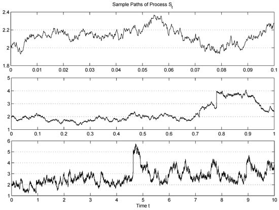
Figure 1.
Sample paths of simulated process for three different time horizons.
For notational simplification, we denote the moments and Laplace transforms by
and the aggregated process by . For the well-posedness of the process, is the stationary condition for the original Hawkes process, and we also need it in some parts of this paper. However, the conventional Feller’s condition for the original CIR process is not required throughout this paper as we allow the process to reach the zero level flexibly.
3. Distributional Properties
Note that this model as defined in Equation (1) is still within the classical affine framework Duffie et al. (2000, 2003). Without losing generality, in this paper, we only consider the canonical case when and for the intensity process in Equation Equation (2), as indeed it is mathematically trivial to derive all associated results below for a general setup based on (see also in Zhu (2014)). Let us first provide the joint Laplace transform of the distribution of :
Proposition 1.
For constants , we have the conditional joint Laplace transform
where is determined by the non-linear ordinary differential equation (ODE)
with the boundary condition ; and is determined by
The proof is provided in Appendix A, which is based on the martingale approach (see also Dassios and Embrechts (1989) and Dassios and Jang (2003)).
Theorem 1.
Under the condition , for any and , the joint Laplace transform of conditional on is given by
where
and is the unique positive solution to the equation .
Proof.
By setting in Equation (4), we have
where is the sigma-algebra generated by , and is uniquely determined by the non-linear ODE
with the boundary condition . Under the condition , it can be solved by the following steps:
- Under the condition of , we havethen, is a strictly decreasing function of . Thus, we have for , since ; there is one unique positive solution to for , and for .
- As should be approachable to zero, we assume , we have and , then, Equation Equation (10) can be written asIntegrate both sides from time 0 to with the initial condition , then we haveDefine the function on the left-hand side asthen, we have ; it is obvious that when .
- By convergence test, we haveObviously, , then,thus when . Therefore, is a well defined (strictly increasing) function and its inverse function exists.
- The unique solution is found by . Hence, .
- Now, is determined byBy the change of variable we have , and
- Finally, substitute and into Equation (8) and the result follows.
□
Corollary 1.
The Laplace transform of aggregated process conditional on is given by
where
Proof.
Setting in Equation (7), the result follows immediately. □
If we set , then , which means that almost surely when .
Note that to derive the Laplace transform of , we cannot trivially set in Equation (7), since does not exist when . Dassios and Zhao (2017a) derived the Laplace transform of and its moments, for which we state the means and variances directly from their results as follows:
Proposition 2.
The expectation of conditional on is given by
where .
Proposition 3.
The variance of conditional on is given by
Similar results for some special cases could also be found in Zhu (2014).
4. Applications
In this section, we first provide an application to insurance for calculating insurance premium by using the moments of from Propositions 2 and 3. We then provide an application to finance for pricing default-free zero-coupon bonds based on Corollary 1.
4.1. An Application in Insurance: Insurance Premium Calculation
We further consider two special cases as below:
- If there are no self-exciting jumps and no diffusion in Equation (12), it becomes a simple Poisson shot-noise process, denoted by , i.e.,This process has been used for actuarial applications as a discounted aggregate loss process, see Jang (2004, 2007) and Jang and Krvavych (2004). If we assume (often implicitly) that interest rate is zero, i.e., , it becomes a simple compound Poisson process .
- If we replace by and set in Equation (12) and , then we have a process ofwith the SDERemark 1.This shot-noise self-exciting jump process in Equation (15) may be interpreted in the context of non-life insurance. A single event (e.g., natural catastrophe) may induce losses for a line of business. Each loss may produce a cluster of losses according to a branching structure (Dassios and Zhao 2011). Both losses are accumulated on a constant risk-free force of interest rate δ.If there are no self-exciting jumps, from Equation (14), we havewith the SDE given bywhich recovers the aggregate loss process used in Jang (2004, 2007).
- In contrast, now let us consider a stochastic interest rate to the aggregate loss amounts up to time t, denoted by , as it is not deterministic in practice. Thus, if we replace by in Equation (12), then we can extend our study from Equations (15) and (16) toRemark 2.This shot-noise self-exciting jump-diffusion process in Equation (17) may be also interpreted in the context of non-life insurance. Similarly, a single event (e.g., a natural catastrophe) may induce losses for a line of business. Compared with Equation (16), both losses are accumulated on a stochastic force of interest rate. The proposed model captures the effect of sudden intensity increases due to external events, together with the accumulation of losses on a stochastic interest rate. Hence, it does have a potential interest in the insurance field.
4.1.1. Expectation of Loss Process
From Proposition 2, by setting and replacing by , the conditional expectation of of Equation (17) is given by
where . We consider two special cases as below:
4.1.2. Variance of Loss Process
Similarly, from Proposition 3, by setting and replacing by , the conditional variance of of Equation (17) is given by
and we consider three special cases as below:
4.1.3. Numerical Examples
Let us illustrate the calculations for the moments of aggregate losses up to time t using the expressions above. For the purpose of illustration, we choose exponential distributions for and , i.e.,
Then, we have their moments and Laplace transforms
We assume that an insurance company’s standard loss frequency rate is 5 per unit time period (say, per year) with the average of losses 1. The mean of after-losses (which are unknown at the arrival times of standard losses from a catastrophic event) is assumed to be 2. We assume that the risk-free force of interest rate is , the volatility is 1, and the initial loss amount that has been carried over is 1. Hence, the parameter values to calculate the moments of aggregate claim amounts are
The calculations of expectations of aggregate loss amounts with stochastic interest rate based on Equations (18)–(20) are shown in Table 1. The calculations of variances of aggregate loss amounts with stochastic interest rate based on Equations (21)–(23) are shown in Table 2.

Table 1.
The expectation of loss: .
Table 2.
The variance of loss: .
Remark 3.
Table 1 and Table 2 show that the expectation and variance of accumulated premium values calculated based on Equations (18) and (21) are much higher than their counterparts calculated based on Equations (19) and (22). This is mainly because they grow exponentially. It becomes much clear if we only consider self-exciting jumps, i.e., given time t, (or, equivalently, ), which is the mean of after-losses, is the main driver to raise the variance of accumulated premium value extremely higher than its counterpart. Hence, the significance of loss-clustering impacts (i.e., after-losses’ impacts) from a catastrophic event depends on after-loss size measure . It would be of interest to examine them using other heavy-tailed distributions for after-loss size measures.
The calculations of variances of aggregate loss amounts with stochastic/deterministic interest rate and their differences by changing the values of diffusion coefficient are shown in Table 3. It is used by Equation (21). The calculations of the moments of aggregate claim amounts by changing the values of for the magnitude of self-exciting jump sizes are shown in Table 4.
Table 3.
The variance of loss: .
Table 4.
Sensitivity analysis of means and variances for the parameter .
Remark 4.
If , the insurance companies have the same variance of aggregate claim amounts even if they consider a stochastic interest rate to the aggregate claim amounts. However, the higher the value of diffusion coefficient is, the higher the variance of aggregate claim amounts is (see Table 3). If insurance companies adopt the mean-variance principle (Bühlmann 1970; Gerber 1979; Goovaerts et al. 1984) for their premium calculations, they become higher than those calculated using a deterministic interest rate. Therefore, it is necessary for insurance companies to charge higher premiums when the interest rate is expected to be more volatile than usual. In addition, as shown in Table 4, the insurance premium charged by mean-variance principle could be very large when after-losses’ impacts (represented by are significant.
4.2. An Application in Finance: Default-Free Bond Pricing
CIR process with externally-exciting and self-exciting jumps presented in the general form of Equation (3) offers a versatile model, interesting both from a theoretical and a practical point view. If we ignore both externally-exciting and self-exciting jumps, it becomes the celebrated CIR model (Cox et al. 1985) for interest rates, denoted by , i.e.,
In this paper, we assume the evolution of interest rate follows this generalised process, i.e., as defined in Equation (1) for any time t. Similar assumptions have been also proposed in Zhu (2014). By setting in Equation (11), we can calculate the prices of default-free zero-coupon bonds paying $1 at time T by
where
We consider two special cases as below:
Numerical Examples
Assume that the frequency rate of externally-exciting events (e.g., news on Greek debt crisis) is 3 per unit time period (say, per year) with their average magnitude of . The mean of self-exciting event (e.g., news of failing to reign in their budget deficits and debts) magnitudes, which are unknown at the arrival times of externally-exciting events, is assumed to be . The risk-free force of interest rate is and that the initial rate of interest is . Hence, the parameter values to calculate the price of a default-free zero-coupon bond are
Table 5.
Bond price .
Using Equation (26), the calculations of bond prices by changing the values of coefficient are shown in Table 6 and Figure 2. Note that, for any time T, when , the unique positive root and , hence, .
Table 6.
Bond price .
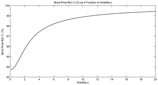
Figure 2.
Bond price (%) as a function of volatility .
Remark 5.
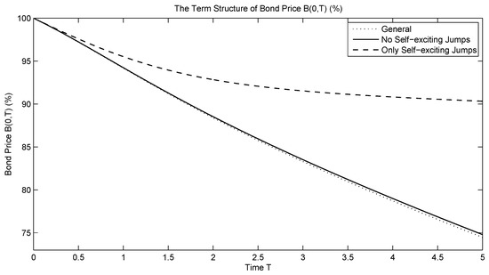
Having considered both the upward externally-exciting and self-exciting jumps in , we are expecting higher interest rates as time goes by. Thus, Table 5 shows that the bond price calculated based on Equation (26) is the lowest. The price calculated based on Equation (28), where only self-exciting jumps are considered, is higher than its counterpart calculated based on Equation (27), as the self-exciting jump frequency rate is lower than the externally-exciting jump frequency rate, (see Figure 3). In addition, the more volatile the interest rate is (meaning more uncertainty for future consumption), the more attractive purchasing a bond that pays guaranteed is. Hence, the higher σ is, the higher the bond price is (see Table 6 and Figure 2), which is the same result as the CIR case.
Figure 3.
Term structure of bond price (%).
The calculations of bond prices by changing the values of and its frequency rate are shown in Table 7 and Table 8, respectively. The bigger the magnitude of positive jumps is, the less attractive purchasing a bond is. Hence, the smaller is, the lower the bond price is (see Table 7). In addition, the higher is, the lower the bond price is (see Table 8).
Table 7.
Sensitivity analysis of bond price for the parameter .
Table 8.
Sensitivity analysis of bond price for the parameter .
We are particularly interested in the special cases where the frequencies and jump sizes are the same, as this would enable us to to compare the effects of self-exciting and externally-exciting jumps. To compare the effect of externally-exciting and self-exciting jumps, we have to make sure that they arrive with an equal frequency on the long run and have the same distribution for their sizes, i.e.,
Table 9.
Bond price .
Remark 6.
Table 9 shows that, if externally-exciting and self-exciting jumps arrive with an equal frequency on the long run and with the same distribution for their sizes, externally-exciting events matter more. We observe that the bond prices calculated based on Equations (26) and (27) are almost the same. Considering only self-exciting events, the bond price calculated based on Equation (28) is higher than its counterpart based on Equation (27). It indicates that their impact on interest rates is not as large as the impact of externally-exciting events. Of course, in practice, it is unlikely that the two kinds of events will arrive with the same frequency and the same distributions of jump sizes; this exercise was to study the impact of the nature of jumps.
5. Conclusions
We studied a generalised CIR process with externally-exciting and self-exciting jumps, and examined the distributional properties. The joint Laplace transform of the process and its integrated process was derived by applying the standard martingale theory. Using the first and second moments of the process, we provided insurance premium calculations and their comparisons with/without self-exciting jumps, and with/without a diffusion coefficient. As a financial application, we present how this Laplace transform can be used for pricing default-free zero-coupon bonds. Numerical calculations for bond prices are illustrated with/without self-exciting jumps, and with/without a diffusion coefficient. Changing the relevant parameters of the process, their sensitivities are also presented for both applications. The estimation exercise for the parameters of this model is important, which is left as future research. Dassios and Zhao (2017a) derived the Laplace transform of and its moments. Maximum likelihood estimation requires the inversion of the Laplace transform for , which is a complicated numerical problem. An alternative is moment-based estimation, where moments can be obtained by successively differentiating the Laplace transform for and indeed the first two are given by Propositions 2 and 3.
Author Contributions
All authors contributed equally to the methodology, analysis and writing of the paper.
Funding
The research of Zhao was funded by National Natural Science Foundation of China grant number 71401147.
Conflicts of Interest
The authors declare no conflict of interest.
Appendix A. Proof for Proposition 1
Proof.
Note that the infinitesimal generator of the joint process acting on a function within its domain is specified by
where is the domain of generator such that is differentiable with respect to z, s and t, and
Consider a function of an exponential affine form , substitute into in Equation Equation (A1), we have
Since this equation holds for any s, it is equivalent to solving two separated equations
With the boundary condition , we have the ODE as Equation (5). By Equation (A2), the integration as Equation (6) follows. Since is a martingale by the property of infinitesimal generator, we have
Then, based on the boundary condition , Equation (4) follows. □
References
- Adamopoulos, L. 1976. Cluster models for earthquakes: Regional comparisons. Journal of the International Association for Mathematical Geology 8: 463–75. [Google Scholar] [CrossRef]
- Aït-Sahalia, Yacine, Julio Cacho-Diaz, and Roger J. A. Laeven. 2015. Modeling financial contagion using mutually exciting jump processes. Journal of Financial Economics 117: 585–606. [Google Scholar] [CrossRef]
- Aït-Sahalia, Yacine, Roger J. A. Laeven, and Loriana Pelizzon. 2014. Mutual excitation in Eurozone sovereign CDS. Journal of Econometrics 183: 151–67. [Google Scholar] [CrossRef]
- Bacry, Emmanuel, Sylvain Delattre, Marc Hoffmann, and Jean-François Muzy. 2013. Modelling microstructure noise with mutually exciting point processes. Quantitative Finance 13: 65–77. [Google Scholar] [CrossRef]
- Bauwens, Luc, and Nikolaus Hautsch. 2009. Modelling financial high frequency data using point processes. In Handbook of Financial Time Series. Edited by Torben G. Andersen, Richard A. Davis, Jens-Peter Kreiß and Thomas Mikosc. Berlin: Springer, pp. 953–79. [Google Scholar]
- Boumezoued, Alexandre. 2016. Population viewpoint on Hawkes processes. Advances in Applied Probability 48: 463–80. [Google Scholar] [CrossRef]
- Bowsher, Clive G. 2007. Modelling security market events in continuous time: Intensity based, multivariate point process models. Journal of Econometrics 141: 876–912. [Google Scholar] [CrossRef]
- Brémaud, Pierre, and Laurent Massoulié. 1996. Stability of nonlinear Hawkes processes. Annals of Probability 24: 1563–88. [Google Scholar]
- Brémaud, Pierre, and Laurent Massoulié. 2001. Hawkes branching point processes without ancestors. Journal of Applied Probability 38: 122–35. [Google Scholar] [CrossRef]
- Brémaud, Pierre, and Laurent Massoulié. 2002. Power spectra of general shot noises and Hawkes point processes with a random excitation. Advances in Applied Probability 34: 205–22. [Google Scholar] [CrossRef]
- Bühlmann, Hans. 1970. Mathematical Methods in Risk Theory. Berlin: Springer-Verlag. [Google Scholar]
- Chavez-Demoulin, Valerie, Anthony C. Davison, and Alexander J. McNeil. 2005. Estimating value-at-risk: A point process approach. Quantitative Finance 5: 227–34. [Google Scholar] [CrossRef]
- Cox, John C., Jonathan E. Ingersoll, Jr., and Stephen A. Ross. 1985. A theory of the term structure of interest rates. Econometrica 53: 385–407. [Google Scholar] [CrossRef]
- Dassios, Angelos, and Paul Embrechts. 1989. Martingales and insurance risk. Stochastic Models 5: 181–217. [Google Scholar] [CrossRef]
- Dassios, Angelos, and Ji-Wook Jang. 2003. Pricing of catastrophe reinsurance and derivatives using the Cox process with shot noise intensity. Finance and Stochastics 7: 73–95. [Google Scholar] [CrossRef]
- Dassios, Angelos, and Hongbiao Zhao. 2011. A dynamic contagion process. Advances in Applied Probability 43: 814–46. [Google Scholar] [CrossRef]
- Dassios, Angelos, and Hongbiao Zhao. 2012. Ruin by dynamic contagion claims. Insurance: Mathematics and Economics 51: 93–106. [Google Scholar] [CrossRef]
- Dassios, Angelos, and Hongbiao Zhao. 2017a. A generalised contagion process with an application to credit risk. International Journal of Theoretical and Applied Finance 20: 1–33. [Google Scholar] [CrossRef]
- Dassios, Angelos, and Hongbiao Zhao. 2017b. Efficient simulation of clustering jumps with CIR intensity. Operations Research 65: 1494–515. [Google Scholar] [CrossRef]
- Duffie, Darrell, Damir Filipović, and Walter Schachermayer. 2003. Affine processes and applications in finance. Annals of Applied Probability 13: 984–1053. [Google Scholar]
- Duffie, Darrell, Jun Pan, and Kenneth Singleton. 2000. Transform analysis and asset pricing for affine jump-diffusions. Econometrica 68: 1343–76. [Google Scholar] [CrossRef]
- Embrechts, Paul, Thomas Liniger, and Lu Lin. 2011. Multivariate Hawkes processes: An application to financial data. Journal of Applied Probability 48A: 367–78. [Google Scholar]
- Errais, Eymen, Kay Giesecke, and Lisa R. Goldberg. 2010. Affine point processes and portfolio credit risk. SIAM Journal on Financial Mathematics 1: 642–65. [Google Scholar] [CrossRef]
- Feller, William. 1951. Two singular diffusion problems. Annals of Mathematics 54: 173–82. [Google Scholar] [CrossRef]
- Gerber, Hans U. 1979. An Introduction to Mathematical Risk Theory. Philadelphia: S.S. Huebner Foundation for Insurance Education. [Google Scholar]
- Goovaerts, Marc J., Florent De Vylder, and Jean Haezendonck. 1984. Insurance Premiums. Amsterdam: North-Holland. [Google Scholar]
- Hawkes, Alan G. 1971a. Point spectra of some mutually exciting point processes. Journal of the Royal Statistical Society. Series B (Methodological) 33: 438–43. [Google Scholar] [CrossRef]
- Hawkes, Alan G. 1971b. Spectra of some self-exciting and mutually exciting point processes. Biometrika 58: 83–90. [Google Scholar] [CrossRef]
- Hawkes, Alan G., and David Oakes. 1974. A cluster process representation of a self-exciting process. Journal of Applied Probability 11: 493–503. [Google Scholar] [CrossRef]
- Jaisson, Thibault, and Mathieu Rosenbaum. 2015. Limit theorems for nearly unstable Hawkes processes. Annals of Applied Probability 25: 600–31. [Google Scholar] [CrossRef]
- Jang, Ji-Wook. 2004. Martingale approach for moments of discounted aggregate claims. Journal of Risk and Insurance 71: 201–11. [Google Scholar] [CrossRef]
- Jang, Ji-Wook. 2007. Jump diffusion processes and their applications in insurance and finance. Insurance: Mathematics and Economics 41: 62–70. [Google Scholar] [CrossRef]
- Jang, Jiwook, and Angelos Dassios. 2013. A bivariate shot noise self-exciting process for insurance. Insurance: Mathematics and Economics 53: 524–32. [Google Scholar] [CrossRef]
- Jang, Ji-Wook, and Yuriy Krvavych. 2004. Arbitrage-free premium calculation for extreme losses using the shot noise process and the Esscher transform. Insurance: Mathematics and Economics 35: 97–111. [Google Scholar] [CrossRef]
- Lando, David. 2004. Credit Risk Modeling: Theory and Applications. Princeton: Princeton University Press. [Google Scholar]
- Léveillé, Ghislain, and José Garrido. 2001. Moments of compound renewal sums with discounted claims. Insurance: Mathematics and Economics 28: 217–31. [Google Scholar]
- Ogata, Yosihiko. 1988. Statistical models for earthquake occurrences and residual analysis for point processes. Journal of the American Statistical Association 83: 9–27. [Google Scholar] [CrossRef]
- Ozaki, Tohru. 1979. Maximum likelihood estimation of Hawkes’ self-exciting point processes. Annals of the Institute of Statistical Mathematics 31: 145–55. [Google Scholar] [CrossRef]
- Stabile, Gabriele, and Giovanni Luca Torrisi. 2010. Risk processes with non-stationary Hawkes claims arrivals. Methodology and Computing in Applied Probability 12: 415–29. [Google Scholar] [CrossRef]
- Vere-Jones, D. 1975. Stochastic models for earthquake sequences. Geophysical Journal International 42: 811–26. [Google Scholar] [CrossRef]
- Vere-Jones, D. 1978. Earthquake prediction—A statistician’s view. Journal of Physics of the Earth 26: 129–46. [Google Scholar] [CrossRef]
- Vere-Jones, D., and T. Ozaki. 1982. Some examples of statistical estimation applied to earthquake data. Annals of the Institute of Statistical Mathematics 34: 189–207. [Google Scholar] [CrossRef]
- Zhu, Lingjiong. 2013a. Central limit theorem for nonlinear Hawkes processes. Journal of Applied Probability 50: 760–71. [Google Scholar] [CrossRef]
- Zhu, Lingjiong. 2013b. Ruin probabilities for risk processes with non-stationary arrivals and subexponential claims. Insurance: Mathematics and Economics 53: 544–50. [Google Scholar] [CrossRef]
- Zhu, Lingjiong. 2014. Limit theorems for a Cox-Ingersoll-Ross process with Hawkes jumps. Journal of Applied Probability 51: 699–712. [Google Scholar] [CrossRef]
- Zhu, Lingjiong. 2015. Large deviations for Markovian nonlinear Hawkes processes. Annals of Applied Probability 25: 548–81. [Google Scholar] [CrossRef]
| 1 | A Markovian Hawkes process is the one with exponential fertility rate. |
| 2 | A similar setup as Equation (2) for constructing dependency between the interest rate and default rate was presented in Lando (2004, p. 123). |
© 2019 by the authors. Licensee MDPI, Basel, Switzerland. This article is an open access article distributed under the terms and conditions of the Creative Commons Attribution (CC BY) license (http://creativecommons.org/licenses/by/4.0/).