
Back-Off Time Calculation Algorithms in WSN


1
Department of Communication Engineering, University of Duisburg-Essen, Duisburg 47057, Germany
2
Department of Computer Science, German University of Technology in Oman, Muscat 111, Oman
3
Department of Computer Science, University of Koblenz, Koblenz 56070, Germany
*
Author to whom correspondence should be addressed.
Informatics 2016, 3(2), 9; https://doi.org/10.3390/informatics3020009
Submission received: 4 March 2016
/
Revised: 16 May 2016
/
Accepted: 12 June 2016
/
Published: 22 June 2016
Abstract
:In a Mobile Wireless Sensor Mesh Network (MWSMN), based on the IEEE 802.15.4 standard, low power consumption is vitally important since the network devices are mostly battery driven. This is especially true for devices dependent on small form factors, such as those used in wireless sensor network. This paper proposes four new approaches to reduce the Back-Off Time in ZigBee standard in order to minimize the collisions caused by transmission between neighbouring nodes within the mesh network. The four alternate algorithms for the Back-Off Time calculation are compared to the ZigBee standard Back-Off Time algorithm regarding their energy needs using the simulation suite OPNET Modeler. To study the behaviour of the parameters of all algorithms in all scenarios, the statistical Analysis of Variance (ANOVA) has been used and it shows that the null hypotheses are rejected except for one case. The results show that the two passive algorithms Tabu Search and Simulated Annealing search techniques are suitable for battery-driven, energy-sensible networks. The Ant Colony Optimization (ACO) approaches increase throughput and reduce the packet loss but cost more in terms of energy due to the implementation of additional control packets. To the best of the authors’ knowledge, this is the first approach for MWSMN that uses the Swarm Intelligence technique and the search solution algorithm for the Back-Off Time optimization.
Keywords:
OPNET Modeler; Zigbee; 802.15.4; Tabu Search; Simulated Annealing; Ant Colony Optimization1. Introduction
The ZigBee standard [1] is a protocol for connecting physically small, low-powered Wi-Fi nodes in a wireless network such as a Mobile Wireless Sensor Mesh Network (MWSMN). The ZigBee standard is based in the IEEE 802.15.4 standard [2]. The physical and the Media Access Layer (MAC) layers are described in the IEEE 802.15.4 standard, while the ZigBee standard is described in the other layers. The term “ZigBee” is trademarked by the ZigBee alliance, which is responsible for the further development of the ZigBee standard [1]. ZigBee is a protocol for wireless medium transmission. Therefore, all sending access by any node to the medium blocks the transmission for all neighbour nodes due to the shared medium. If any neighbour node tries to send information at the same time, it will block the transmission of the first node and makes a collision. This makes collisions a bigger problem than in a wired network, where usually the medium is not shared (exceptions, such as the Token Ring network or the use of hubs have existed, but are not commonly used at this time).
Wireless media is a broadcast media, which means a single sending station saturates the entire channel. At the same time, all stations receive all packets sent. If two or more stations try to send data at the same time, the packets are damaged (a collision happens) and need to be resent causing degradation of the efficiency. To minimize the number of collisions, the Collision Sense-Multiple Access (CSMA) protocol was designed [3]. Instead of transmitting as soon as a packet is ready to be sent, the station first listens on the common media to detect whether or not there is already a packet being transmitted. However, collisions can still occur if two stations simultaneously start to send packets, or if, due to propagation delay, a station senses an empty channel, even though another station has already begun sending.
One mechanism to minimize the number of collisions and therefore improve the efficiency of the network is the use of a Back-Off Time algorithm [2]. When a node cannot send a packet because the medium is already in use, it waits for a certain amount of time, which is randomly determined instead of trying again instantly. This time span is called the “Back-Off Time”. In the IEEE 802.15.4 standard, the Back-Off period is the time a station waits after it has sensed a full channel before it tries again. While the exact calculation of the length of this Back-Off period depends on the exponential Back-Off period (at first the maximum period is short, but it is then lengthened every time the station senses a full channel), there is always a random factor involved so as to avoid deadlocks. In the standard ZigBee algorithm, the maximum value of this Back-Off Time increases each time the node fails to send its packet. Back-Off Time is a random number between one time unit and 127 time units and is not directly scaling with regards to the environmental conditions (such as average packet length, increases or decreases in traffic or the addition of new nodes to the network), but is calculated only according to the number of failed communication attempts [4].
The goal of this paper is to propose new Back-Off mechanisms based on the Swarm Intelligence (SI) technique [5,6] and the Search solution algorithm based on Tabu Search [7] in order to lower power consumption, increase throughput and decrease delay times in MWSMN. The new algorithms consider additional data such as the behaviour of neighbouring nodes or previous environmental situations. The new algorithms have been divided into two parts: passive and active algorithms. The active algorithm depends on the node status and shares some information about the node itself to the neighbouring nodes, while the passive algorithms do not support this function. To the best of the authors’ knowledge, this is the first approach for MWSMN that uses the Swarm Intelligence techniques and the search solution algorithm for the Back-Off Time optimization in MWSMN.
2. Alternative Back-Off Time Algorithms
In this paper, a deeper introduction into the alternate mechanisms, which are usually used for finding local optimums in a group of solutions, are used for the calculation of the Back-Off Time algorithm. There is a certain challenge in adapting these approaches, which try to find the best possible solution in a certain amount of time for an unchanging problem to a problem field in which the fitness of the solutions changes over time, as network traffic can increase or decrease according to external influences. The following approaches are used as bases for the algorithms tested.
2.1. Tabu Search Approach
The Tabu Search is one of the optimizing localized search algorithms [7]. Moreover, the Tabu Search algorithm is very important and used to enhance the local search performance in order to find an improved solution. The idea behind this algorithm is to mark certain potential solutions as “taboo” if they have already been visited so that these solutions are not considered again or if they have been declared as unsuitable in order to guarantee the termination of the search algorithm. Evaluated results are stored in the “Tabu List”. Some variations of this algorithm are to store undesirable solutions in this list so that these are under no circumstances considered. For example, assuming the Tabu Search is applied to the Travelling Salesman Problem (TSP) where certain arcs are prohibited to ease the calculation, excluding certain routes in advance would be possible. Tabu Search is the basis for one of the alternate Back-Off mechanisms examined in this work.
Considering the fluctuating nature of the wireless system, there is no such solution as a “best” Back-Off Time; thus, instead of letting the algorithm decide a certain Back-Off Time, it is more suitable to let it decide the best interval with the specific Back-Off Time being chosen randomly from this interval. The Tabu Search approach used in this work is very simple and serves primarily as a test bed: the Back-Off Time is divided into five intervals. One of those is chosen randomly. The actual Back-Off Time is then picked randomly from within the chosen interval. As soon as a new Back-Off period is needed, another Back-Off interval is chosen. This new Back-Off interval, however, cannot be the same as the previous one. Tabu Search in this work keeps a memory list of one formerly used solution. These solutions are not visited again for a time N, where N is the size of the memory list. This means that the same solution interval is never chosen twice in a row. Considering the small solution space (five, in this case), a longer memory could prove disadvantageous.
Figure 1 represents the Back-Off Time optimization based on the Tabu Search. According to the Institute of Electrical and Electronics Engineers (IEEE) Computer Society [2], the maximal Back-Off Time exponent in the standard ZigBee Back-Off mechanism is five; therefore, the possible maximum Back-Off Time is 255 time units. This maximum Back-Off Time is, in this work, separated into five intervals: (1–51), (52–102), (103–153), (152–204), and (205–255). The only important change for the Tabu Search approach is exchanging the Back-Off Time calculation algorithm. Instead of increasing the maximum Back-Off Time when a communication attempt fails, in the Tabu Search approach, this is avoided by the Back-Off Time being divided into five intervals. Since the maximum Back-Off Time in the ZigBee protocol is 255 time units, each interval is comprised of 51 time units. For example, if the third of these intervals is active, the Back-Off Time, which is still chosen randomly by the network node, would be between 102 and 153 time units. If a communication attempt fails, which means a Back-Off period needs to be calculated, another interval is activated. The Back-Off Time is then randomly chosen from the active interval; in the above example, a possible Back-Off Time would be 143 time units. This algorithm is primarily a proof-of-concept; therefore, this algorithm was designed to be as simple as possible, even though this limits its practical use. For convenient calculation, the intervals are numbered 0 to 4; this eases defining the maximum and minimal Back-Off Time for each interval.
In this work, the memory space is exactly one solution. This memory space is filled with one randomly chosen interval. Then, whenever a Back-Off Time is required, a solution interval is chosen randomly. If this random interval is not the interval in memory, this becomes the Back-Off Time. Then, the interval’s identifier is saved in the memory, overwriting the old one and freeing it for future use. Otherwise, another random interval is selected.
Given the five intervals I1 to I5, we pre-load the memory space with I4. Then, a Back-Off Time is needed as the node detects that the channel is in use. The new randomly selected solution interval is I1; this interval is not I4, so it is a valid solution. Therefore, a Back-Off Time is randomly selected from (1–51) time units and I1 is stored in the memory space. Later on, another Back-Off Time is needed. This time, the randomly selected interval is I1; however, since I1 is also the last chosen interval, this solution is discarded and another interval, in this round I3, is selected. The Back-Off Time is then chosen from (102–153) time units and I3 is stored in the memory space. This frees up I1 as a valid solution again.
2.2. Simulated Annealing Approach
Simulated Annealing is an optimization approach that is based on the annealing process in metallurgy. In addition, the Simulated Annealing algorithm is used in large discrete search space in order to find an optimum solution for a given problem with a target proposal. The first approach is still rather simple. This simplicity allows for less power consumption during calculation and requires little memory on the network node, but it can also lead to suboptimal solutions. In order to shorten the time between sent packets while still ensuring a minimum of collisions, the Back-Off Time algorithm considers the environment, namely, how many other stations are active and how saturated the channel is. This approach considering environmental behaviour is based on the Simulated Annealing technique—as the metal is heated and cooled countless times until the atoms are in the best position—so the chosen Back-Off interval is switched between neighbouring solutions depending on the traffic. Each node distributes its traffic dates, which are the number of date packets, to the neighbouring nodes because the node with the highest number of date packets is given the highest priority to send by assigning the least Back-Off Time. Thus, first, the number of date packets per node is calculated and distributed and then checked to determine whether or not the data packages are ready to be sent. Finally, the channel will be checked. If it is free from interference, the data packets are sent. If the channel is already being used by another node, a Back-Off Time is assigned.
The Simulated Annealing describes a process of continuing improvement for the search space. The search space is seen as the state of a physical object. The best possible results are seen as those states with the lowest internal status. In each iteration, the neighbouring solutions of the one actual chosen are considered and they are chosen with a probability depending on their status. This allows this algorithm to overcome local optimized results, but makes finding the best solution improbable. Therefore, this algorithm is best suited for finding a solution that is acceptable.
The Back-Off Time optimization based on the Simulated Annealing algorithm is depicted in Figure 2. This approach is adapted to be the “Counting Packets” approach. The maximum Back-Off Time is divided into several possible solution intervals from which the current Back-Off Time will be drawn. Each time a Back-Off Time is necessary, the traffic since the last time a Back-Off Time was necessary is compared to the traffic in the period before that and, according to this comparison, the chosen solution interval is adapted. If the traffic has lessened during this last period, an interval containing smaller Back-Off Times is chosen; if it has increased, an interval will be chosen which contains longer Back-Off Times.
In this approach, after a temporary solution has been chosen, the neighbouring solutions are considered. Depending on the fitness function, if a certain threshold is crossed, one of these neighbouring solutions may become the new temporary solution. If there is no solution that crosses the threshold, the algorithm terminates and returns the temporary solution.
In this approach, external data are considered for the calculation of the Back-Off Time. In order to perform this calculation, the number of packets received for a given time span are counted (which, since ZigBee is a broadcast medium, are all packets sent in the vicinity of the node) and compared to the number of packets sent in another time span, t − 1. If the traffic has increased, the Back-Off Time is increased in order to lower the load on the channel. Similarly, if less traffic has been sent, the Back-Off Time can be decreased.
Then, according to this information, a new Back-Off interval is chosen; first, it is checked to determine as to whether or not there has been an increase or decrease in network traffic since the last invocation of the Back-Off Time scheduling function. If there has been an increase, a Back-Off interval with longer Back-Off Times will be chosen, should the interval not already be at the maximum value; likewise, if there has been a decrease, the Back-Off Time will also decrease, but only if the interval is not already at its lowest possible value.
The minimum Back-Off period of 52 time units was chosen deliberately—this guarantees that the node listens long enough to form a correct opinion about the state of traffic before it reconsiders its choice. Then, the Back-Off period is randomly determined from the freshly chosen Back-Off interval.
2.3. Ant Colony Optimization Approach
The Ant Colony Optimization (ACO) algorithm was primarily designed to find optimal routes between a central station (the anthill) and outlying sensor nodes. The ACO technique is used to solve the computational problems by finding the best optimum solutions for target problems. This makes the algorithm extremely suitable for route discovery in wireless sensor networks in which sensor nodes deliver their data to the central data sink [8]. The optimization in this algorithm is done via so-called pheromone updates—the more autonomous agents (the ants) use a given trail, consider it a good one and tag it with its pheromone, the more autonomous agents will use that certain route. In real life, each ant simply tags all paths it traverses. If a path can be traversed faster, which is the metric by which ants measure the fitness, the round trip time between the ant hill and the goal is shorter.
For example, consider there are two paths between the anthill and a food source, and path A can be traversed in half the time the trip via path B would take. Then, if one ant each would travel via each path, then the ant which travels on path A would complete two trips in the time the other ant would complete one trip, and thus would also tag the first route twice as often. In the next iteration of the decision process, both ants would then choose to travel via path A.
For calculating the optimal Back-Off Time, an adapted approach is used. The maximum Back-Off Time supported by ZigBee is divided into several intervals. Instead of tagging a route, a Back-Off interval is tagged, and, depending on the fitness evaluation, the nodes calculate their preferred Back-Off interval from the information their neighbouring nodes publicize about their current situation.
The ACO algorithm is one of the SI techniques [9]. This technique suffers from a similar problem as the other optimization approaches: there is no best result, since the shortest Back-Off Time is dependent on the situation. Instead, the best interval for the Back-Off Time needs to be chosen regularly. In this paper, two options for an ACO Back-Off Time algorithm are evaluated.
The most complex approach considered is an implementation of the Ant Colony Optimization algorithm. Instead of only listening passively to incoming data like in Simulated Annealing approach, the nodes themselves give out information about their preferred Back-Off Time. This allows other nodes to evaluate the current situation by choosing their Back-Off intervals according to these “tags”. The Ant Colony Optimization has two variants: “Normal” uses the most often tagged interval, while the “Inverse” Ant Colony Optimization variant uses the least often tagged interval instead.
2.3.1. Choosing the Most Often Used Interval
Ant Colony Optimization is a path-finding algorithm based on the behaviour of ants. It is also the foundation of one of the alternate Back-Off Time mechanisms examined in this work.
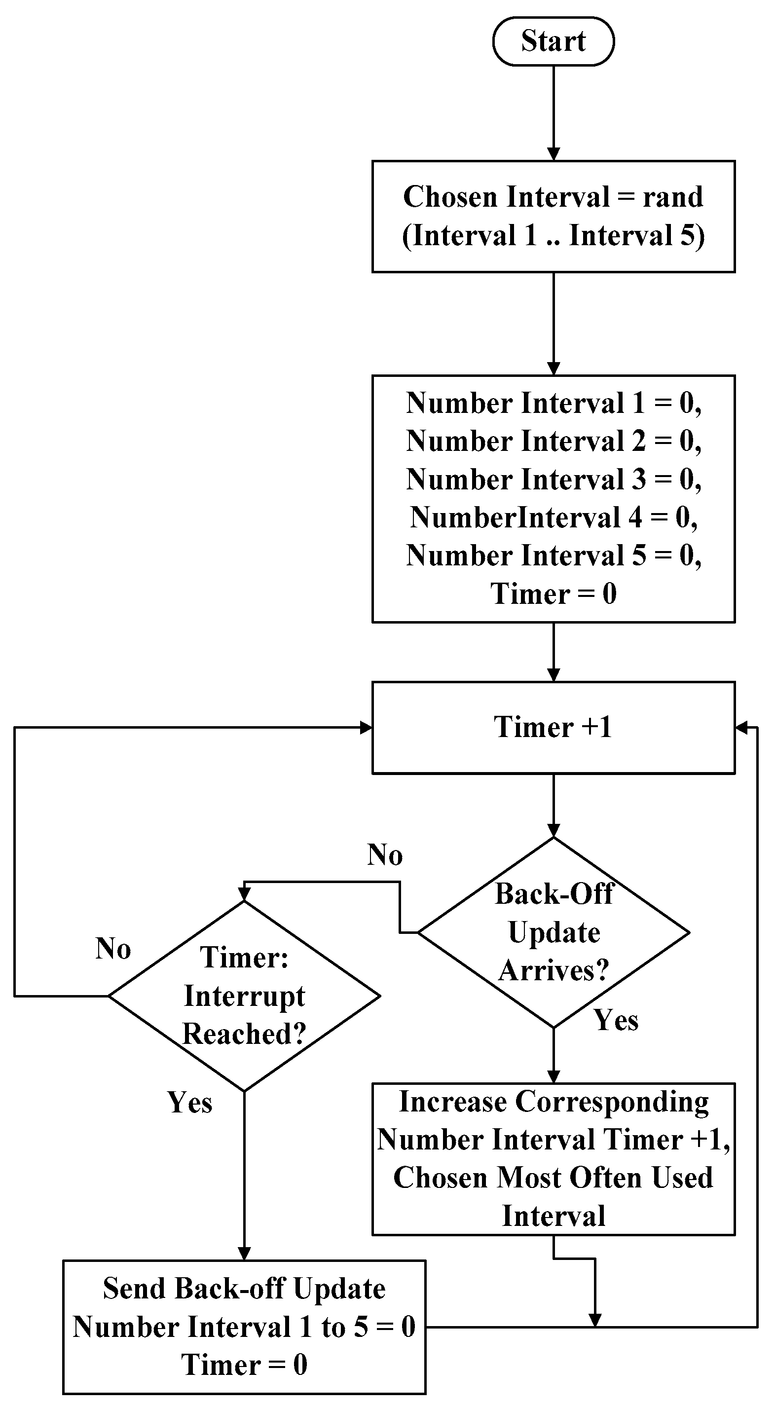
The Ant Colony approach is based on tagging “the best route”—in this case, it means tagging a certain interval for the Back-Off Time. In this approach, the participating stations send their chosen interval, which is chosen randomly, over the control channel, after a certain time. If the nodes succeed in sending this update message, it implies that the chosen interval must be adequate. Therefore, if more stations use a certain interval and are successful, more stations will switch to that interval. Given the five defined intervals in Section 2.1, a possible implementation of this algorithm is presented in Figure 3.
In order to prevent the stations from choosing a suboptimal interval, there needs to be a random chance of switching to another interval.
Given the five intervals, a basic idea of this algorithm could be as per the following two options: each packet includes the chosen Back-Off Time interval. Packets with well-chosen intervals are sent sooner and are therefore more frequent; therefore, these intervals are transmitted more often and appear in higher counts. This leads to a preference for that Back-Off Time interval, which simulates the pheromone effect.
For the Ant Colony Optimization approach, huge changes have to be performed. Since this approach is a proactive one in which each node periodically broadcasts an update to its neighbour nodes about its preferred Back-Off Time interval, a new packet format needs to be designed to transport this additional information and the new packet needs to be as small as possible so it does not congest the channel (since ZigBee is a wireless protocol, all access is automatically broadcast access and blocks all other access to the shared medium). Furthermore, it must be made sure that it is possible for the node to filter out its own sent update packets so the node does not consider its own internal data.
2.3.2. Choosing the Unused Intervals
Another option for the ACO would be to choose the least often chosen interval. This has two advantages over the first approach.
- It does not converge on a single interval, ensuring that the algorithm remains flexible enough to adapt to new nodes joining the network.
- Since the least often used interval is chosen, the channel is probably free after the interval has passed.
Given the five defined intervals in Section 2.1, a possible implementation of this algorithm is presented in Figure 4. This approach is adapted as an Inverse Ant Colony Optimization (ICAO).
The difference between this method and the previous one is only in the Back-Off Time selection. After the Timer reaches 50, the Back-Off Time update arrives. Thus, a new Back-Off Time interval must be selected. In this method, the least often used interval (most often not used interval) for the Back-Off Time is selected in order to reduce the collisions since it has not been selected by the neighbouring nodes, while in the previous method that is also based on ACO, the Back-Off Time is selected with the most often used interval due to its success to send date by the neighbouring nodes. It can be clearly seen that this algorithm is almost completely identical to the one deployed in the normal ACO algorithm.
As discussed in Section 2.3.1, the changes that are necessary for the inverse Ant colony Optimization approach are for the most part identical to the changes necessary for the normal Ant Colony Optimization approach. However, the incoming Back-Off Time update packets must be processed differently. Instead of choosing the most used interval for the Back-Off Time calculation, the algorithm decides to pick the least commonly used interval. This prevents stagnation, i.e., the nodes preferred choice changes over time and adapts to the actual situation, which should ensure a network that never converges on a single, suboptimal interval. For this reason, the approach is called “Inverse” Ant Colony Optimization—because it behaves exactly diametrically opposed to the natural ant colony behaviour.
Whether these algorithms are effective or not, and if they are, then to what degree, is demonstrated in next section.
3. Simulation Results
OPNET 16 simulator has been used to evaluate the network performance [10]. OPNET Modeler is a network simulation suite capable of simulating ZigBee traffic that offers a wide selection of built-in measurements for discrete event simulation. Many modelling profiles in OPNET Modeler have been used to implement these algorithms. These modelling profiles are Network Model, Node Model, Process Model, Link Model, Application Profile, and Mobility Profile [10]. In addition, there is Carrier Sense Multiple Access (CSMA) Algorithm for reducing the interferences, which contains the CSMA/Collision Avoidance (CA), and the Unslotted (Beacon-less) CSMA/CA. Examination of all offered variables would consume too many resources. Instead, a relevant subgroup will be chosen in order to maximize gathered knowledge while minimizing the needed number of evaluated variables.
3.1. Simulation Metrics
The most important parameter is energy consumption; after that, are the usual Quality-of-Service parameters such as delay and throughput.
- Additional management traffic: ZigBee traffic uses a wireless medium. Each transmission of data blocks the medium for all other nodes. In order to minimize collisions, the amount of control traffic sent must be minimized. In addition, additional traffic puts more strain on the device’s power supply. Since most ZigBee devices are battery driven, with the capacity of batteries being small [8], this is an especially important aspect for a Wireless Sensor Network (WSN) protocol because the energy consumption depends mainly on the traffic sent. While a passive node still uses battery power, this consumption is far smaller than the energy needed to actively send data since the amount of payload data sent does not depend on the algorithm. Only the MAC management traffic is dependent on the algorithm, so the lesser the management traffic, the better the algorithm, especially since management traffic can lead to collisions or to data not arriving at a network node because of an event in which the target node is sending a management package at the same point in time. Management traffic is measured in bits per second.
- Throughput: A higher throughput means that, if the other factors are identical, one given algorithm is more efficient at data transmission. A high throughput is most important in the cases in which large amounts of data are transported. This allows either for more devices to be deployed in the same area or more data can be sent by the devices (for example, in a medical use case, there could be additional safeguards that the data transmitted are correct). If the control traffic used by the protocol becomes too large, throughput—and therefore usability—is lowered. Throughput can be measured in a Discrete Event Simulation (DES) directly by OPNET Modeler’s board tools. Throughput is measured in bits per second.
- Delay: It is the trip time between a node being ready to send a packet and a packet being sent. In order to gain knowledge about this, trip time needs to be analysed. A large discrepancy between those two points of time would mean that data sent may be out of context or obsolete by the time they are read by the receiving station. This is especially important in time-critical applications such as health monitoring or financial applications. OPNET Modeler is capable of monitoring delay with its board tools. Depending on the use case, short delays on the MAC layer might be necessary in order to guarantee the data processed are up-to-date. Delay is measured in seconds.
- Traffic Dropped: packet loss is also an important factor of measurement. Each packet that is dropped because of collisions and full queues in the destination node needs to be resent, thus increasing the energy cost for the sending node and both lowering throughput (each dropped packet blocks the channel at least for a short time) and also increasing the delay (a packet that arrives later). While this additional delay may not be important in most use cases, they could be critical in others. The integrated tools of Modeler can capture the number of dropped packets. Traffic Dropped is measured in bits per second.
3.2. Simulation Result
In order to test the different Back-Off Time algorithms described Section 2, their efficiency and their power drain will be simulated in different scenarios. In this paper, four scenarios are presented. In order to understand the simulation result, a brief explanation is given for each scenario because the nodes number, mobility, and distribution affect the result.
Network and geographical topologies are depicted in OPNET Modeler using Scenarios. A scenario consists of the network nodes, the connections between these nodes and a geographical background in which the topology is situated (for instance, an office block or a transcontinental network). Optionally, subnets, a mobility configuration and application configurations can be included. The scenarios are chosen to demonstrate the alternate Back-Off Time algorithms that are explained in the previous sections.
Since Zigbee nodes can be small and lightweight, they can be used in highly mobile use cases such as access control schemes or theft alarms in supermarkets. OPNET Modeler offers the possibility to assign a mobility configuration to a scenario that describes the pattern in which the node’s movements shall be calculated during simulation. OPNET Modeler offers several built-in algorithms for this, for example random waypoint model.
A DES has been used, which is a simulation in which each incident is recreated. This is in contrast to other kinds of simulations, which would only use average values over time. This makes DES a very granular kind of simulation. The following results were recorded over a simulated time period of one hour in all scenarios except “Randomized”, where, due to the higher number of nodes and the corresponding higher computational cost, a time period of only fifteen minutes was chosen. Each scenario is run ten times for each approach. These runs differed in the “seed value” that initialized the simulation’s random number generator [10]. The seed value is the initialization point of a pseudo random number generator. If all seeds are known, the behaviour of such an algorithm can be predicted. These seed values were chosen randomly themselves in order to decouple the results from external influences and quirk events in as best a way as possible. For each run, there is a different seed value. They are, however, the same for all scenarios and algorithms so as to facilitate the comparison of the collected data.
The results given here are always the average results over the entire network for each run. They are given in US-American notation, i.e., with a “,” for each thousand and a point as the decimal separator key, as this is the standard output of OPNET Modeler.
The goal of this work was the evaluation of the different Back-Off Time algorithms in order to lower power consumption, increase throughput and decrease delay times.
3.2.1. Simple Scenario
The Simple scenario serves in theory only as a function test. In other words, The “Small Test Area” scenario is the basic test bed for the algorithms. The objective here is to check the correctness of the alternate Back-Off Time algorithms. Therefore, the network topology is fairly simple: four sensors, eight routers and one end node (sink node) that collects the data sent by the sensors. In this case, the routers are fixed sensors, which also function as routers for the mobile sensors. All doors, for example, could be equipped with motion detectors that notify the alarm system in the event of somebody gaining unlawful entry. The mobile sensors could represent four guards, who each patrol a certain area of the building and are carrying a panic button. The panic button and the other sensors not only send a distress call when they are triggered, but also send regular status messages in order to prevent an attack on the infrastructure; they do this by jamming the signal or destroying the sensor. The nodes are all configured as belonging to Wireless Personal Area Network (WPAN) and all send their data to the “Data Sink” node, with the exception of the data sink itself—its purpose is only to evaluate the data. The mobile configuration is that sensors may move up to two metres from their starting point. One thousand twenty-four bits of payload are sent once per second to the data sink from each sensor and router, simulating a regular update.
However, the data gathered can also be used to infer the performance of the algorithms in small networks. Considering a possible deployment example for a real-life application (an office security system), low energy cost would be a paramount measuring value for this scenario. The following tables represent the results for alternate the Back-Off Time calculation algorithm and the standard ZigBee algorithm.
ZigBee Standard
ZigBee is a communications protocol based on the IEEE 802.15.4 standard. It focuses primarily on small, low-power devices. The most popular applications for ZigBee are wireless sensor networks. The ZigBee approach in Table 1 is the base line for all other approaches. The strength of this scenario is the low delay. Its drawback lies in the number of dropped packets because the nodes do not take any information about the status of the neighbouring nodes. This makes this approach especially suited for small amounts of data that need to be communicated as fast as possible.
Tabu Search
The Tabu Search approach in Table 2 offers similar amounts of management traffic sent and a similar throughput. However, it is far slower with regard to delay (roughly five times as long) and it has a far better rate regarding packets dropped—less than two per cent of the amount of data dropped compared to the ZigBee standard implementation because the Back-Off Time is reduced by making five intervals. Additionally, in half of the runs of this scenario, no data were dropped at all. Depending on the use case, this may well outweigh the longer delay. In a small home alarm system, for example, where the lower number of packets is dropped, the power cost is lowered and the live time of a battery-powered motion detector is increased, thus far exceeding the value of triggering an alarm fifty milliseconds earlier.
Counting Packets
The Counting Packets results in Table 3 are close to the Tabu Search; however, they are in all aspects worse—only slightly worse, but noticeably so due to a new parameter that has been used. The advantages and weaknesses with regard to the ZigBee standard implementation stay the same: fewer dropped packets means less power consumption, while higher delay times reduce the usability in low latency use cases.
Ant Colony Optimization
The advantages of the ACO approaches run in an entirely different direction (Table 4). While the average throughput is comparable to the other approaches in this scenario, the number of dropped packets is, about half the time, astoundingly high (roughly 120 times the rate of the standard scenario), and the management traffic sent is higher by about 60 bits/s; the delay is remarkably low—about half the time needed compared to the standard implementation and about one-tenth of the time needed compared to the Counting Packets and the Tabu Search approaches. Additionally, in four of the runs, the number of packets dropped is lower than in the standard implementation. Apparently, using these seeds as a basis for the random number generator, the algorithm is capable of finding an optimum solution.
As can be seen, the algorithm simply chooses the most popular interval. This correlates to the natural ant colony behaviour in which ants choose the path most often used. This means that, in theory, the algorithm should converge sooner or later on an optimal interval. However, this is actually not the case; most of the time, the nodes converge on a suboptimal interval, which leads to packet loss and therefore to higher energy consumption. This is true for the others scenario.
Inverse Ant Colony Optimization
In Table 5, the DES simulation runs for the Inverse ACO (IACO) approach have roughly the same results as those for the normal ACO approach because the same technique has been used, even if it is the inverse one but still working for the small number of nodes. The average values are better, but not by so much that it really makes a difference.
3.2.2. Randomized Scenario
The “Randomized Test Area” is similar to the “Small Test Area” scenario—a scenario designed primarily for testing the algorithms. Instead of a small, planned network, however, this scenario was created randomly using the “Rapid Configuration” feature of OPNET Modeler 16.0. This feature allows the fast creation of large networks (in this scenario 150 nodes) without considerable effort. The Randomized scenario is a pure stress test for the algorithms. Designed only to check the robustness in large and homogeneous networks, throughput and packet losses are important statistics, while energy consumption is not nearly as important as in most other scenarios. In this scenario, there are 150 nodes compared to few nodes (less than 10 nodes) in the previous scenario, so the simulation result will be different. Again, there is a single Data Sink node; all other nodes are configured to send data to the sink. The sending interval is normally distributed with a mean outcome of 0.25 and a variance of 0.5. Since this scenario served as a test bed for large configurations, these nodes—although capable of mobility—are not configured to move. Additionally, due to the large computational cost of this scenario, the runtime of this scenario is only fifteen minutes, not an hour as with all other scenarios.
ZigBee Standard
The standardized Back-Off Time mechanism suffers when the network becomes bigger due to the passive technique that has been used because the nodes depend on themselves only without considering any other parameter to select the Back-Off Time. For the first attempt to send data packets, the Back-Off Time is chosen from the small interval of time, with a large amount of (active) nodes, the probability that two nodes try to send at the same time is rather high. In Table 6, this can be seen clearly in the increase of MAC delay (up to 0.0141 s, which is 1.5 times higher than in the simple scenario) and the increase in lost packets. However, the algorithm is, with regard to throughput, still rather efficient.
Tabu Search
In the Randomized scenario, the Tabu Search approach in Table 7 is generally worse than the ZigBee standard implementation. It has longer delays (six times longer, which is an even greater difference than in the Simple scenario); it has lower throughput (only about 84 per cent of the standard algorithm’s throughput); and required about 200 bits/s more management traffic. However, the number of dropped packets is still extremely low. This again makes this approach useful for systems in which throughput and delay are secondary to energy concerns because this algorithm is based on a passive technique.
Counting Packets
The result in Table 8 for the Counting Packets approach is again similar to the Tabu Search results. However, in this scenario, they are better with shorter delay time; a higher throughput, fewer packets dropped because of the usage of the new parameter, which is about the traffic form the neighbouring nodes; and only a marginally higher amount of MAC management traffic sent. Again, these values suggest that this approach could be useful in use cases where the delay is less important than low power consumption.
Ant Colony Optimization
The ACO approach in Table 9 also continues its trend—high throughput (twice as much as the next non-ACO based approach), low delay times (0.06 s—half as much as the ZigBee standard algorithm) and astonishingly high amounts of dropped traffic. The dropped traffic outnumbers the transported data by a ratio of roughly 3:1. This means that in large networks, this approach suffers strongly due to the need to send additional data, unlike the passive algorithms (Tabu, Zigbee standard, and Counting Packet approaches), which can gather all the needed information without having to add to the network’s load. This limits the use of this approach in battery-powered nodes.
Inverse Ant Colony Optimization
The IACO results in Table 10 again shares the characteristics of the normal ACO approach because it is an active algorithm, unlike the passive algorithms. Therefore, the possible use cases are likewise limited to scenarios in which energy consumption is a negligible priority, but throughput needs to be guaranteed.
3.2.3. Patient Bed Scenario
This commonly used scenario is the so-called “Wireless Body Area Network” (WBAN) [11]. WBANs are most commonly used in the medical field. In this scenario, reliability, little energy consumption and low delay times are most important. However, the mobility of the sensors is so limited that it may as well be ignored. Three such WBAN are simulated in the “Patient Bed” scenario. Considering the fact that the data about the patient have to be up to date almost instantly, this scenario uses a mean update interval for the sensors of one second. Additionally, one of the most important differences of this scenario compared to others is the fact that there are three data sinks, which are deployed in close physical proximity to simulate possibly overlapping networks, each sink with its six sensors (as in first scenario, few nodes per sink). The simulated location—a patient room in a hospital—is taken from the “Office” network scale, sized 15 × 15 m2. The first two scenarios (Simple and Randomized) all utilize only one personal area network, while the Fire House scenario has greater physical separation between the two floors. The ZigBee topology chosen for this scenario is a meshed network. The data sinks only collect data, but do not generate traffic themselves.
ZigBee Standard:
The ZigBee standard approach is a very good fit for this scenario because of the small number of nodes. In Table 11, low delay time combined with little management traffic and an acceptable number packets dropped reduce the power consumption while still vouching for accurate and fast data transmission.
Tabu Search
The Tabu Search approach, from the measurements alone in Table 12, is still a useful alternative compared to the ZigBee standard approach because of the small number of nodes in this scenario. While the delay is still far higher, the fewer dropped packets may make up for it, depending on whether energy consumption or fast message transfer is more desirable. However, the more complex the scenarios become, the worse this approach fares in comparison to the other newly designed passive algorithm, the Counting Packets approach.
Counting Packets
The Counting Packets approach firmly places itself as one of the two best approaches for this scenario, the other being the ZigBee standard approach, because it uses the information coming from the neighbouring nodes to choose the best Back-Off Time interval. The measured values in Table 13 are better than in the Tabu Search approach (except for the management traffic sent, but the difference there is only 4 bits/s), especially considering the extremely low number of dropped packets. This algorithm proves itself to be ideal for a low-energy scenario. An example for such a scenario could be a field hospital in a disaster area, where, due to limited resources, a longer battery life is more important than an immediate update.
Ant Colony Optimization
The ACO approaches are not suited for this kind of deployment. In Table 14, besides the high number of packets dropped (but again, in only half of the runs), the amount of management data is increased due to the regular sending of the Back-Off Time updates that need to be sent for this approach to work. In the ACO approaches, the throughput is worse than the other approaches; that is, only half as much as for the three passive approaches, but its strength is the extremely short delay times. While such an arrangement may be suitable in other scenarios, it is not a feasible approach as soon as low energy consumption is one of the main requirements. The fact that three independent WBANs are deployed next to each other appears to be the main source of these approaches’ problems, as in no other scenario are they so prominent.
Inverse Ant Colony Optimization
The IACO, as shown in Table 15, fares only a little better than the normal variant. The short delay simply cannot compete with the large number of packets dropped and the small amount of throughput due to the sending of additional control packets.
3.2.4. Fire Station Scenario
The “Fire Station” scenario is the second real-world application. It simulates a smart fire watch house with several sensors, for example, whether the water tanks on the fire engine are full, what the status of the equipment is and so forth, which helps make maintenance easier and further helps to ensure mission readiness. This scenario has been modelled to simulate a modern, medium-sized fire station. The fire station itself has two floors, each spanning their own network. On the upper floor, there are the sleeping arrangements for the fire fighters on watch, a cafeteria/kitchen and the command centre from which possible deployments are handled. Also modelled on the upper floor are two fire fighters who are on duty.
On the lower floor, the fire engines are stored—in this example, there are three of them—as well as the hose workshop, in which the fire hoses are cleaned, dried, repaired, stored and inspected. Then there is the clothing chamber (which works as a lock; fire-fighters fresh from a deployment can change in there without bringing dirt or hard-to-remove particles of soot into the rest of the station).
These fire fighter nodes are the only mobile nodes in this scenario, as all other nodes are either fixed (such as the status indicators for the clothing chamber) or relatively immobile (such as the fire engines; while these are certainly mobile, this work assumes that there is no deployment over the course of the simulated one-hour time period).
The Fire Station scenario has the largest number of nodes of all planned scenarios. This is reflected in the high throughput. Additionally, due to the large number of nodes, active algorithms (ACO and IACO) have to contend with a large increase in management traffic.
The Fire Station network is updated irregularly; the sensors mostly send data when there has been a new development, as well as sending status updates. This is simulated by choosing a constant packet size (1024 bits, which should be large enough for such specialized sensors) and a normal distribution for the packet inter-arrival time. The application traffic starts at 55 s of simulated time and is continued until the end of the simulation. This late start was chosen due to the rather large number of nodes, the ZigBee network was not completely formed at the standard start time for application traffic.
Standard ZigBee
The Standard ZigBee implementation in Table 16 offers a high throughput in this scenario. The MAC layer delay is considerably larger than in the smaller networks (roughly 1.2 times as long). This result is in agreement with other published works [12]. It also shows the necessity of implementing new mechanisms for collision avoidance in such densely populated networks, depending on the performance requirements.
Tabu Search
The Tabu Search approach in Table 17 is again similar in performance to the ZigBee standard approach, sacrificing delay times for fewer packets dropped. This confirms the results of all other scenarios. However, this approach is not recommended by its measurement values, since the Counting Packets approach is, simply said, better.
Counting Packets
The Counting Packets approach again establishes itself as the approach that is best for the low energy consumption, while it retains a high throughput. The long delays, however, may be problematic for certain parts of this scenario (such as the clothing chamber’s lock). The results in Table 18 of this scenario also show again that, in medium to large networks, the Counting Packets approach is superior to the Tabu Search approach.
Ant Colony Optimization
In Table 19, the data point that stands out the most in the results of the Fire House scenario is the large amount of dropped data—5300 bits/s are dropped—which is more than five times as many as are dropped in the ZigBee standard results shown in Table 16. In addition, there is no run in which the amount of data dropped is significantly lower, which leads to the conclusion that at least in this scenario the ACO algorithm appears to be unable to calculate an optimal interval. In Addition to this problem, the management traffic in this mechanism is again higher than in the passive approaches, and this is why we have a large amount of dropped data. This, in combination with the lower throughput, makes it apparent that the ACO approach is not suitable for this scenario, even though the MAC delay is, again, very short.
Inverse Ant Colony Optimization
The IACO approach in Table 20 (as with the ACO one) is similarly unsuited for this scenario (for the task of being used in a smart fire house) due to the high number of packets dropped and the management traffic. While the measured values are better than those of the normal ACO algorithm, the improvement is so small. It can be easily tracked back to chance (i.e., under these certain seed values, the Inverse ACO algorithm is better, but if another batch of seed values would be determined randomly, the normal ACO algorithm might deliver better results).
3.2.5. Comparison of Average Values
In order to better visualize the different strength of the algorithms, their performance for each of the measurement values are compared directly.
The clearly best algorithms regarding MAC delay in Table 21 are the ACO and IACO approaches. Each has a MAC delay that is at least 0.004 s better than the second best algorithm. Additionally, these algorithms scale extremely well; the average delay time is always around 0.005 s, whereas all other approaches need longer times that are proportionate to the size of the network. This is especially apparent in the Counting Packets approach and the Tabu Search approach, where the delay in the largest network is roughly double the delay in the Simple scenario.
For degradation performance in terms of throughputs in Table 22, a different picture can be shown. The three passive approaches offer higher values, with the standard implementation offering the highest rates in the Simple scenario and the Counting Packets approach being the best in the Patient Bed and Fire House scenarios. An exception is the Randomized scenario, in which the throughput of the ACO-based approaches is roughly 1.8 times that of the passive approaches.
In Table 23, the number of dropped packets in the passive algorithms clearly outperforms the ZigBee standard implementation as well as the ACO approaches. This makes these algorithms suitable for any use case in which low energy consumption is key and trumps any other concerns such as throughput or delay.
As the ACO approaches broadcast regular updates of their state, it is only natural that they need to send more management traffic. As a result in Table 24, more data than the Counting Packets approach drop in that rather large scenario. As for the passive approaches, they tend to be rather close with each other, with the ZigBee standard implementation being the best in most cases.
3.2.6. Comparisons between Algorithms and Scenarios using ANOVA
It is worth mentioning that the practical results presented in Table 1 and Table 2 are not compared precisely. In order to study the behaviour of the parameters of algorithms in all scenarios, the so-called statistical Analysis of Variance (ANOVA) [13] needs to be applied for each algorithm and scenario. In fact, ANOVA is usually used for comparison between the performances of variables/parameters (more than 2). Moreover, ANOVA compares the variation of the performance of variables/parameters by splitting the total variations into two components, between the group means and the variation within the groups, and finally showing if this variation is significant or not.
In addition, ANOVA is either a parametric or non-parametric test based on available observations. In this paper, a non-parametric test is performed and preferred because of the number of observations in each algorithm (if the sample size <30 observation). The non-parametric test is applied in two directions, as follows:
- a.
- The comparisons are among the parameters of each algorithm for all the scenarios.
The null hypothesis of the above task is defined as the following: the medians of Parameters are the same across algorithms (non-parametric test).
Using statistical package IBM SPSS-20 [11], the final results of the test are very big and, in order to save space, the significance levels of the hypotheses are given for each approach and parameter as shown in Table 25.
Table 25 shows that the values of all significance levels are 0.000, i.e., the null hypotheses are rejected (theoretically the significance level for rejecting each null hypothesis should be less than 0.05 [11,13]), i.e., there is a significant difference between the values of each parameter per algorithm/scenario.
- b.
- The comparisons are among the parameters of each scenario for different algorithms.
The Null Hypothesis of the second task is defined as the following: the medians of parameters are the same cross scenarios (non-parametric test).
Using the same statistical package, IBM SPSS-20, the final results of the above test are given in Table 26.
Table 26 shows that the null hypotheses are rejected except for the throughput at the Simple Scenario; we think the reason is because of fewer nodes.
4. Conclusions
Four alternate Back-Off Time optimization algorithms for MWSMN, based on IEEE 802.15.4 standard, were proposed. We compared our proposed algorithms with the standard Back-Off Time algorithm in four scenarios. The experimental results gathered in the scenarios have led to several clear conclusions. In addition, ANOVA has been used to study the behaviour of the parameters of all algorithms in all scenarios and shows that the null hypotheses are rejected for all of the cases except for one, which is when we have compared the throughput of different algorithms in the simple scenario.
The standard ZigBee Back-Off Time algorithm is a good all-round mechanism, excelling in the area of low delay, and is especially suited for small networks; the bigger a network becomes, the longer the delays become and the more packets will be dropped en-route.
The two passive algorithms, Tabu Search and Counting Packets (the latter of which is based on the Simulated Annealing search technique), can also be very useful. Because few, if any, packets are lost while retaining most of the performance of the standard algorithm, beating it even, except for the delay time, these algorithms are suitable for battery-driven, energy-sensible networks. It is notable, however, that in all but one scenario the Counting Packets approach outperforms the Tabu Search approach.
The ACO approaches solved the problem with an active approach. The additional control packets required cost power, which in a device with a small form factor, may be limited. Additionally, a node sending its control packet is not open for receiving data. This led to dropped packets, which in turn required even more power. These problems are most prominent in large networks. However, the low delay times and the fact that the normal ACO approach sometimes converges on a good interval, reducing the number of lost packets and increasing throughput, should also be mentioned.
Considering the fact that the two more successful approaches were the Tabu Search approach and the Counting Packets approach, more research could be invested in these two algorithms for future work. For example, in the Tabu Search approach, a longer memory in combination with a greater number of intervals could improve the efficiency.
In this paper, the numerical results of all algorithms and scenarios are compared using ANOVA tests. It is particularly interesting to observe that most of the null hypotheses are rejected (except one), i.e., we can report that most of the algorithms and scenarios are significant. The logical interpretation/justification of this result is as per the following statement: there are significant differences between scenarios due to the parameters of algorithms.
To the best of the authors’ knowledge, this is the first approach on MWSMN that uses the Swarm Intelligence Technique (ACO and IACO) and the search solution algorithm (Tabu Search and Simulated Annealing) for the Back-Off Time optimization.
Acknowledgments
The authors would like to thank Francis Andrew, College of Applied Science, Nizwa, Oman for proofreading the paper.
Authors Contributions
Ali Al-Humairi has conceived and designed the experiments; Alexander Probst has performed the experiments; Ali Al-Humairi and Alexander Probst have analysed the data; Ali Al-Humairi has contributed analysis tools and written the paper.
Conflicts of Interest
The authors declare no conflict of interest.
References
- Zigbee Alliance. Available online: http://www.zigbee.org (accessed on 17 June 2016).
- IEEE Standards Association. IEEE Get Program Computer Society IEEE Standard 802.15.4. Available online: http://standards.ieee.org/getieee802/download/802.15.4-2006.pdf (accessed on 29 September 2011).
- Andrew, S. Tanenbaum Computer Networks, 4th ed.; Prentice Hall: Upper Saddle River, NJ, USA, 2003. [Google Scholar]
- 802.15.4-2006-IEEE Standard for Information Technology. Available online: http://standards.ieee.org/findstds/standard/802.15.4-2006.html (accessed on 29 September 2015).
- Abraham, A.; He, G.; Liu, H. Swarm intelligence: Foundations, perspectives and applications. In Swarm Intelligent Systems; Springer: Berlin/Heidelberg, Germany, 2006. [Google Scholar]
- Zhang, Y.; Agarwal, P.; Bhatnagr, V. Swarm Intelligence and Its Applications 2014. Sci. World J. 2014, 2014. [Google Scholar] [CrossRef] [PubMed]
- Glover, F.; Laguna, M. Tabu Search; Kluwer Academic Publishers: Dordrecht, The Netherlands, 1997. [Google Scholar]
- Schurgers, C.; Srivastava, M.B. Energy efficient routing in wireless sensor networks. In Proceedings of the MILCOM 2001 Communications for Network-Centric Operations: Creating the Information Force, Fairfax, VA, USA, 28–31 October 2001.
- Saleem, M.; di Caro, G.A.; Farooq, M. Swarm intelligence based routing protocol for wireless sensor networks: Survey and future directions. Inform. Sci. 2011, 181, 4597–4624. [Google Scholar] [CrossRef]
- OPNET. Modeler Manual Built-in Manual for OPNET Modeler; OPNET: Bethesda, MD, USA, 2011. [Google Scholar]
- IBM SPSS Software. Available online: http://www.ibm.com/analytics/us/en/technology/spss/ (accessed on 1 May 2015).
- Bianchi, G. Performance Analysis of the IEEE 802.11 Distributed Coordination Function. IEEE J. Sel. Areas Commun. 2000, 18, 535–547. [Google Scholar] [CrossRef]
- Sabine, L.; Brian, S.E. A Handbook of Statistical Analyses Using SPSS; Chapman & Hall: Boca Raton, FL, USA, 2004. [Google Scholar]
Figure 1.
Back-Off Time Optimization based on the Tabu Search Algorithm.

Figure 2.
Back-Off Time Optimization based on the Simulated Annealing Algorithm.

Figure 3.
Back-Off Time Optimization based on the Ant Colony Optimization Algorithm (Used Interval).
Figure 3.
Back-Off Time Optimization based on the Ant Colony Optimization Algorithm (Used Interval).

Figure 4.
Back-Off Time Optimization based on the Ant Colony Optimization Algorithm (Unused Intervals).
Figure 4.
Back-Off Time Optimization based on the Ant Colony Optimization Algorithm (Unused Intervals).


| RUN | MAC Delay | Throughout | Packets Dropped | Management Traffic |
|---|---|---|---|---|
| 1 | 0.008968 | 16,009.77 | 0.02116 | 1.0646 |
| 2 | 0.008924 | 15,963.99 | 0.178 | 8.94 |
| 3 | 0.009420 | 17,025.86 | 66.42 | 8.15 |
| 4 | 0.008988 | 15,967.10 | 3.418 | 8.15 |
| 5 | 0.009438 | 15,963.84 | 7.289 | 8.82 |
| 6 | 0.009547 | 15,968.06 | 8.10 | 9.14 |
| 7 | 0.008859 | 15,963.70 | 0.898 | 10.33 |
| 8 | 0.008851 | 15,968.76 | 0.987 | 8.08 |
| 9 | 0.008629 | 15,969.49 | 1.440 | 9.88 |
| 10 | 0.008942 | 15,962.76 | 2.071 | 8.42 |
| AVG | 0.009057 | 16,076 | 9.08 | 8.13 |
| RUN | MAC Delay | Throughout | Packets Dropped | Management Traffic |
|---|---|---|---|---|
| 1 | 0.04771 | 15,964.79 | 0.00 | 8.74 |
| 2 | 0.04869 | 15,985.28 | 0.00 | 8.48 |
| 3 | 0.04670 | 15,971.43 | 0.00 | 9.40 |
| 4 | 0.04967 | 15,970.20 | 0.0889 | 8.55 |
| 5 | 0.04876 | 15,975.66 | 0.00 | 8.55 |
| 6 | 0.04655 | 15,970.52 | 0.0889 | 9.28 |
| 7 | 0.00885 | 15,963.70 | 0.898 | 10.33 |
| 8 | 0.05040 | 17,107.40 | 0.453 | 8.08 |
| 9 | 0.04900 | 15,970.76 | 0.0 | 8.75 |
| 10 | 0.04810 | 15,970.52 | 0.0889 | 8.02 |
| AVG | 0.04446 | 16,085 | 0.16 | 8.84 |
| RUN | MAC Delay | Throughout | Packets Dropped | Management Traffic |
|---|---|---|---|---|
| 1 | 0.04812 | 15,964.18 | 0.182 | 8.74 |
| 2 | 0.04881 | 15,975.10 | 0.0889 | 8.48 |
| 3 | 0.04707 | 15,971.43 | 0.00 | 8.34 |
| 4 | 0.04684 | 15,984.35 | 0.00 | 8.68 |
| 5 | 0.04891 | 15,970.52 | 0.0889 | 9.08 |
| 6 | 0.04748 | 15,964.65 | 0.0889 | 9.61 |
| 7 | 0.04743 | 15,971.08 | 0.00 | 8.08 |
| 8 | 0.04743 | 15,971.08 | 0.00 | 8.08 |
| 9 | 0.4835 | 15,971.08 | 0.00 | 8.08 |
| 10 | 0.04704 | 15,965.52 | 0.00 | 9.14 |
| AVG | 0.04774 | 15,970 | 045 | 8.63 |
| RUN | MAC Delay | Throughout | Packets Dropped | Management Traffic |
|---|---|---|---|---|
| 1 | 0.005155 | 17,076.62 | 5.48 | 67.62 |
| 2 | 0.005155 | 13,662.30 | 1291.38 | 68.26 |
| 3 | 0.005152 | 17,077.08 | 5.39 | 67.25 |
| 4 | 0.005155 | 17,068.22 | 7.18 | 70.07 |
| 5 | 0.005156 | 14,793.06 | 1293.02 | 67.33 |
| 6 | 0.005150 | 14,696.82 | 1294.82 | 68.81 |
| 7 | 0.005150 | 17,079.75 | 1292.30 | 67.73 |
| 8 | 0.005154 | 15,940.60 | 6.65 | 68.20 |
| 9 | 0.005155 | 13,662.30 | 1291.38 | 68.26 |
| 10 | 0.005157 | 14,790.76 | 1294.91 | 67.76 |
| AVG | 0.005120 | 15,594 | 778 | 68.13 |
| RUN | MAC Delay | Throughout | Packets Dropped | Management Traffic |
|---|---|---|---|---|
| 1 | 0.005158 | 17,068.68 | 7.28 | 68.80 |
| 2 | 0.005156 | 17,065.06 | 5.12 | 69.00 |
| 3 | 0.005152 | 17,073.58 | 6.47 | 67.08 |
| 4 | 0.005159 | 17,066.83 | 7.18 | 69.31 |
| 5 | 0.005156 | 14,792.74 | 1291.94 | 70.28 |
| 6 | 0.005150 | 14,800.31 | 1293.74 | 68.89 |
| 7 | 0.005150 | 17,076.89 | 1291.94 | 67.40 |
| 8 | 0.005154 | 15,942.51 | 3.41 | 68.79 |
| 9 | 0.005156 | 13,660.08 | 1293.90 | 69.87 |
| 10 | 0.005157 | 14,793.30 | 1293.47 | 69.87 |
| AVG | 0.00520 | 15,933 | 649 | 68.92 |
| RUN | MAC Delay | Throughout | Packets Dropped | Management Traffic |
|---|---|---|---|---|
| 1 | 0.01409 | 39,039.87 | 6252.49 | 1999.77 |
| 2 | 0.01413 | 36,966.35 | 6553.44 | 2000.14 |
| 3 | 0.01428 | 34,359.29 | 6535.16 | 2097.17 |
| 4 | 0.01430 | 38,786.04 | 6568.14 | 1915.17 |
| 5 | 0.01412 | 39,476.12 | 6506.22 | 2041.72 |
| 6 | 0.01425 | 34,758.62 | 6457.26 | 2048.36 |
| 7 | 0.01413 | 35,825.89 | 6589.44 | 1910.49 |
| 8 | 0.01425 | 34,844.26 | 6577.92 | 1953.99 |
| 9 | 0.01405 | 39,052.29 | 6651.36 | 2287.25 |
| 10 | 0.01406 | 38,951.96 | 6578.22 | 2086.17 |
| AVG | 0.01418 | 37,206 | 6526 | 2034 |
| RUN | MAC Delay | Throughout | Packets Dropped | Management Traffic |
|---|---|---|---|---|
| 1 | 0.08554 | 31,448.97 | 999.36 | 2036.00 |
| 2 | 0.08329 | 32,928.87 | 974.88 | 2265.32 |
| 3 | 0.08395 | 32,751.16 | 1104.48 | 2300.76 |
| 4 | 0.08316 | 32,640.80 | 1088.64 | 2389.90 |
| 5 | 0.08437 | 28,332.54 | 1048.32 | 2157.03 |
| 6 | 0.08325 | 30,572.76 | 1061.28 | 2431.41 |
| 7 | 0.08416 | 30,394.49 | 959.34 | 2334.11 |
| 8 | 0.08480 | 30,321.02 | 1081.44 | 2301.71 |
| 9 | 0.08452 | 26,898.44 | 1090.08 | 2544.76 |
| 10 | 0.08428 | 27,754.18 | 1080.00 | 2230.03 |
| AVG | 0.08415 | 30,504 | 1.049 | 2299 |
| RUN | MAC Delay | Throughout | Packets Dropped | Management Traffic |
|---|---|---|---|---|
| 1 | 0.07767 | 31,363.07 | 879.84 | 2221.08 |
| 2 | 0.07719 | 33,844.28 | 826.56 | 2325.64 |
| 3 | 0.07775 | 27,593.62 | 849.60 | 2423.86 |
| 4 | 0.07829 | 27,365.02 | 797.76 | 2265.99 |
| 5 | 0.07694 | 32,444.25 | 823.68 | 2357.85 |
| 6 | 0.07767 | 32,229.30 | 879.84 | 2096.37 |
| 7 | 0.07783 | 31,460.48 | 861.12 | 2211.54 |
| 8 | 0.07677 | 33,350.88 | 819.36 | 2706.54 |
| 9 | 0.07836 | 25,987.68 | 858.24 | 2105.50 |
| 10 | 0.07764 | 32,623.40 | 802.08 | 2583.47 |
| AVG | 0.07762 | 30,826 | 839 | 2330 |
| RUN | MAC Delay | Throughout | Packets Dropped | Management Traffic |
|---|---|---|---|---|
| 1 | 0.00618 | 54,872.43 | 143,539.6 | 2479.25 |
| 2 | 0.00615 | 57,883.83 | 145,789.9 | 2353.99 |
| 3 | 0.00618 | 59,881.74 | 145,611.2 | 2494.86 |
| 4 | 0.00618 | 62,100.44 | 145,336.9 | 2498.08 |
| 5 | 0.00615 | 61,405.67 | 147,265.2 | 2560.59 |
| 6 | 0.00614 | 60,448.79 | 146,409.4 | 2368.00 |
| 7 | 0.00619 | 57,883.62 | 144,154.2 | 2440.09 |
| 8 | 0.00619 | 56,877.57 | 146,064.7 | 2224.80 |
| 9 | 0.00620 | 53,436.81 | 143,960.7 | 2627.80 |
| 10 | 0.00619 | 56,597.92 | 143,693.5 | 2346.83 |
| AVG | 0.0062 | 58,138 | 145,182 | 2439 |
| RUN | MAC Delay | Throughout | Packets Dropped | Management Traffic |
|---|---|---|---|---|
| 1 | 0.006192 | 55,130.46 | 144,366.1 | 2486.01 |
| 2 | 0.006157 | 57,761.80 | 146,578.3 | 2351.63 |
| 3 | 0.006188 | 59,764.80 | 147,353.6 | 2489.80 |
| 4 | 0.006189 | 62,575.83 | 145,970.5 | 2481.19 |
| 5 | 0.006152 | 60,939.17 | 146,545.2 | 2562.95 |
| 6 | 0.006155 | 59,944.16 | 144,999.6 | 2345.55 |
| 7 | 0.006188 | 57,893.79 | 145,726.6 | 2421.42 |
| 8 | 0.006199 | 56,736.48 | 145,991.2 | 2209.90 |
| 9 | 0.006202 | 53,683.40 | 144,666.3 | 2610.58 |
| 10 | 0.006199 | 56,454.28 | 144,308.4 | 2338.38 |
| AVG | 0.0062 | 58,088 | 145,660 | 2430 |
| RUN | MAC Delay | Throughout | Packets Dropped | Management Traffic |
|---|---|---|---|---|
| 1 | 0.01068 | 38,562.44 | 954.44 | 16.28 |
| 2 | 0.01024 | 39,836.10 | 99.35 | 18.00 |
| 3 | 0.01115 | 42,335.76 | 732.49 | 17.79 |
| 4 | 0.01112 | 37,680.49 | 774.88 | 18.32 |
| 5 | 0.01038 | 44,728.92 | 540.44 | 17.40 |
| 6 | 0.01109 | 37,680.13 | 498.85 | 17.00 |
| 7 | 0.00975 | 38,864.41 | 44.34 | 19.19 |
| 8 | 0.01000 | 38,750.99 | 102.22 | 16.41 |
| 9 | 0.01176 | 37,752.16 | 829.04 | 19.73 |
| 10 | 0.01063 | 38,064.18 | 598.30 | 17.60 |
| AVG | 0.01069 | 39,359 | 517 | 17.77 |
| RUN | MAC Delay | Throughout | Packets Dropped | Management Traffic |
|---|---|---|---|---|
| 1 | 0.05830 | 39,936.06 | 36.53 | 15.48 |
| 2 | 0.06992 | 42,027.86 | 210.68 | 17.35 |
| 3 | 0.05749 | 39,938.03 | 49.50 | 16.12 |
| 4 | 0.05427 | 38,813.15 | 20.88 | 17.07 |
| 5 | 0.05763 | 37,690.84 | 46.97 | 16.21 |
| 6 | 0.05824 | 42,188.40 | 95.12 | 15.74 |
| 7 | 0.05582 | 40,015.86 | 37.62 | 20.17 |
| 8 | 0.05933 | 39,902.42 | 88.83 | 16.87 |
| 9 | 0.06014 | 38,803.08 | 110.25 | 18.00 |
| 10 | 0.05996 | 38,824.87 | 93.96 | 105.77 |
| AVG | 0.05910 | 39,818 | 79 | 25.8 |
| RUN | MAC Delay | Throughout | Packets Dropped | Management Traffic |
|---|---|---|---|---|
| 1 | 0.05298 | 40,974.57 | 8.280 | 94.41 |
| 2 | 0.06992 | 40,959.82 | 2.25 | 21.15 |
| 3 | 0.05289 | 40,976.78 | 6.840 | 20.88 |
| 4 | 0.05291 | 40,969.71 | 10.800 | 20.94 |
| 5 | 0.05144 | 40,981.59 | 0.360 | 20.21 |
| 6 | 0.05545 | 40,923.74 | 66.96 | 22.74 |
| 7 | 0.05318 | 40,960.73 | 30.24 | 23.46 |
| 8 | 0.05727 | 51,014.36 | 205.92 | 22.00 |
| 9 | 0.05184 | 40,971.81 | 10.529 | 21.60 |
| 10 | 0.05146 | 30,691.96 | 50.7639 | 21.54 |
| AVG | 0.055 | 40,942 | 39 | 29 |
| RUN | MAC Delay | Throughout | Packets Dropped | Management Traffic |
|---|---|---|---|---|
| 1 | 0.005164 | 20,470.42 | 4.78 | 141.49 |
| 2 | 0.005164 | 19,332.47 | 1292.97 | 140.05 |
| 3 | 0.005165 | 19,330.72 | 1292.70 | 144.89 |
| 4 | 0.005163 | 17,060.45 | 3865.89 | 145.84 |
| 5 | 0.005164 | 19,328.49 | 1293.13 | 16.21 |
| 6 | 0.005163 | 20,467.24 | 5.88 | 142.56 |
| 7 | 0.005165 | 20,468.32 | 4.24 | 140.83 |
| 8 | 0.005164 | 20,467.67 | 2.98 | 145.14 |
| 9 | 0.005164 | 18,193.64 | 2580.72 | 142.77 |
| 10 | 0.005163 | 19,329.96 | 1288.11 | 149.88 |
| AVG | 0.0052 | 19,445 | 1163 | 131 |
| RUN | MAC Delay | Throughout | Packets Dropped | Management Traffic |
|---|---|---|---|---|
| 1 | 0.005169 | 19,335.28 | 1290.60 | 115.33 |
| 2 | 0.005167 | 21,084.47 | 2012.87 | 122.71 |
| 3 | 0.005170 | 20,467.97 | 8.01 | 112.86 |
| 4 | 0.005168 | 19,336.88 | 1289.97 | 114.50 |
| 5 | 0.005169 | 19,335.74 | 1292.58 | 115.02 |
| 6 | 0.005169 | 20,469.68 | 3.151 | 115.91 |
| 7 | 0.005169 | 19,338.13 | 1290.69 | 112.03 |
| 8 | 0.005169 | 20,474.20 | 2.249 | 115.46 |
| 9 | 0.005168 | 18,203.77 | 2597.76 | 115.81 |
| 10 | 0.005169 | 20,474.96 | 3.693 | 117.21 |
| AVG | 0.0052 | 17,917 | 977 | 116 |
| RUN | MAC Delay | Throughout | Packets Dropped | Management Traffic |
|---|---|---|---|---|
| 1 | 0.01004 | 51,993.67 | 744.84 | 39.92 |
| 2 | 0.00999 | 51,933.42 | 740.88 | 48.67 |
| 3 | 0.01001 | 53,270.60 | 738.36 | 39.32 |
| 4 | 0.00997 | 51,910.66 | 771.48 | 44.77 |
| 5 | 0.01012 | 55,206.34 | 860.40 | 41.84 |
| 6 | 0.01001 | 52,934.64 | 826.92 | 45.81 |
| 7 | 0.01047 | 51,948.61 | 767.88 | 44.08 |
| 8 | 0.01014 | 54,961.14 | 908.64 | 45.36 |
| 9 | 0.01008 | 51,903.67 | 741.24 | 44.51 |
| 10 | 0.01102 | 53,940.48 | 987.48 | 40.51 |
| AVG | 0.01018 | 53,000 | 809 | 43 |
| RUN | MAC Delay | Throughout | Packets Dropped | Management Traffic |
|---|---|---|---|---|
| 1 | 0.06044 | 52,631.38 | 243.36 | 42.50 |
| 2 | 0.06056 | 52,602.63 | 244.44 | 37.86 |
| 3 | 0.05928 | 52,633.04 | 240.12 | 39.38 |
| 4 | 0.05928 | 52,583.88 | 192.96 | 42.51 |
| 5 | 0.06040 | 52,664.10 | 255.96 | 40.65 |
| 6 | 0.06234 | 53,725.41 | 290.16 | 44.50 |
| 7 | 0.05949 | 52,671.22 | 228.24 | 44.68 |
| 8 | 0.05871 | 52,768.23 | 189.00 | 48.27 |
| 9 | 0.05911 | 52,690.05 | 189.36 | 43.17 |
| 10 | 0.05884 | 52,768.66 | 143.64 | 37.85 |
| AVG | 0.06011 | 52,773 | 221 | 42 |
| RUN | MAC Delay | Throughout | Packets Dropped | Management Traffic |
|---|---|---|---|---|
| 1 | 0.05363 | 53,910.12 | 108.00 | 54.16 |
| 2 | 0.05506 | 53,880.85 | 175.68 | 40.57 |
| 3 | 0.05278 | 55,196.40 | 47.88 | 43.16 |
| 4 | 0.05392 | 54,955.27 | 109.80 | 47.16 |
| 5 | 0.05384 | 53,854.68 | 164.16 | 44.10 |
| 6 | 0.05358 | 53,953.82 | 119.52 | 40.65 |
| 7 | 0.05240 | 53,949.94 | 81.72 | 42.70 |
| 8 | 0.05379 | 53,992.59 | 147.24 | 48.15 |
| 9 | 0.05443 | 53,873.04 | 145.08 | 42.97 |
| 10 | 0.05443 | 53,974.19 | 154.08 | 43.43 |
| AVG | 0.05380 | 54,154 | 125 | 44 |
| RUN | MAC Delay | Throughout | Packets Dropped | Management Traffic |
|---|---|---|---|---|
| 1 | 0.005223 | 44,798.76 | 5857.56 | 186.85 |
| 2 | 0.005223 | 46,626.72 | 4882.32 | 180.71 |
| 3 | 0.005226 | 44,188.51 | 6247.44 | 184.70 |
| 4 | 0.005223 | 46,964.87 | 4719.24 | 182.16 |
| 5 | 0.005220 | 46,387.75 | 5030.72 | 186.85 |
| 6 | 0.005224 | 44,628.73 | 6072.56 | 189.10 |
| 7 | 0.005224 | 46,182.50 | 5253.20 | 189.52 |
| 8 | 0.005224 | 44,942.50 | 5893.20 | 184.78 |
| 9 | 0.005223 | 46,199.76 | 5091.99 | 191.34 |
| 10 | 0.005223 | 47,463.14 | 4497.12 | 184.96 |
| AVG | 0.00522 | 45,837 | 5355 | 186 |
| RUN | MAC Delay | Throughout | Packets Dropped | Management Traffic |
|---|---|---|---|---|
| 1 | 0.005224 | 44,695.48 | 5809.68 | 168.94 |
| 2 | 0.005225 | 46,438.60 | 4947.12 | 181.39 |
| 3 | 0.005227 | 44,188.51 | 6295.68 | 182.34 |
| 4 | 0.005225 | 47,029.38 | 4744.80 | 180.80 |
| 5 | 0.005224 | 46,617.29 | 5082.92 | 184.49 |
| 6 | 0.005226 | 46,251.46 | 6103.52 | 188.51 |
| 7 | 0.005225 | 46,251.46 | 5224.04 | 193.49 |
| 8 | 0.005224 | 44,849.71 | 5921.28 | 180.13 |
| 9 | 0.005223 | 46,243.73 | 5119.35 | 187.03 |
| 10 | 0.005224 | 47,599.47 | 4360.68 | 185.47 |
| AVG | 0.0052 | 45,839 | 5361 | 185 |
| Approach | Simple Scenario | Random | Patent Bed | Fire Station |
|---|---|---|---|---|
| ZigBee Standard | 0.009 | 0.014 | 0.011 | 0.010 |
| Tabu Search | 0.044 | 0.084 | 0.059 | 0.060 |
| Counting Packets | 0.048 | 0.077 | 0.055 | 0.053 |
| ACO | 0.005 | 0.006 | 0.005 | 0.005 |
| IACO | 0.005 | 0.006 | 0.005 | 0.005 |
| Approach | Simple Scenario | Random | Patent Bed | Fire Station |
|---|---|---|---|---|
| ZigBee Standard | 16,076 | 37,2068 | 39,359 | 53,000 |
| Tabu Search | 16,085 | 30,504 | 39,818 | 52,773 |
| Counting Packets | 15,970 | 30,826 | 40,942 | 54,154 |
| ACO | 15,594 | 58,138 | 19,445 | 45,837 |
| IACO | 15,933 | 58,088 | 17,918 | 45,839 |
| Approach | Simple Scenario | Random | Patent Bed | Fire Station |
|---|---|---|---|---|
| ZigBee Standard | 9.08 | 6525 | 517 | 809 |
| Tabu Search | 0.16 | 1049 | 79 | 221 |
| Counting Packets | 0.45 | 839 | 39 | 125 |
| ACO | 778 | 145,182 | 1163 | 5355 |
| IACO | 649 | 145,660 | 977 | 5361 |
| Approach | Simple Scenario | Random | Patent Bed | Fire Station |
|---|---|---|---|---|
| ZigBee Standard | 8.13 | 2034 | 17.77 | 43 |
| Tabu Search | 8.84 | 2299 | 25.8 | 42 |
| Counting Packets | 8.63 | 2330 | 29 | 44 |
| ACO | 68.13 | 2439 | 131 | 186 |
| IACO | 68.92 | 2430 | 116 | 185 |
| Approach | Number of Parameters | MAC Delay | Management Traffic | Packets Drop | Throughput |
|---|---|---|---|---|---|
| ACO | 4 | 0.000 | 0.000 | 0.000 | 0.000 |
| Counting Packets | 4 | 0.000 | 0.000 | 0.000 | 0.000 |
| IACO | 4 | 0.000 | 0.000 | 0.000 | 0.000 |
| Tabu Search | 4 | 0.000 | 0.000 | 0.000 | 0.000 |
| Zigbee | 4 | 0.000 | 0.000 | 0.000 | 0.000 |
| Scenario | Number Of Algorithms | MAC Delay | Management Traffic | Packets Drop | Throughput |
|---|---|---|---|---|---|
| Simple | 5 | 0.000 | 0.000 | 0.000 | 0.128 |
| Randomized | 5 | 0.000 | 0.000 | 0.000 | 0.000 |
| Patient Bed | 5 | 0.000 | 0.048 | 0.000 | 0.000 |
| Fire Station | 5 | 0.000 | 0.000 | 0.000 | 0.000 |
* The standard significance levels value is equal to 0.05.
© 2016 by the authors; licensee MDPI, Basel, Switzerland. This article is an open access article distributed under the terms and conditions of the Creative Commons Attribution license ( http://creativecommons.org/licenses/by/4.0/).
Share and Cite
MDPI and ACS Style
Al-Humairi, A.; Probst, A. Back-Off Time Calculation Algorithms in WSN. Informatics 2016, 3, 9. https://doi.org/10.3390/informatics3020009
AMA Style
Al-Humairi A, Probst A. Back-Off Time Calculation Algorithms in WSN. Informatics. 2016; 3(2):9. https://doi.org/10.3390/informatics3020009
Chicago/Turabian StyleAl-Humairi, Ali, and Alexander Probst. 2016. "Back-Off Time Calculation Algorithms in WSN" Informatics 3, no. 2: 9. https://doi.org/10.3390/informatics3020009
Note that from the first issue of 2016, this journal uses article numbers instead of page numbers. See further details here.