Big Data Management with Incremental K-Means Trees–GPU-Accelerated Construction and Visualization

Abstract

While big data is revolutionizing scientific research, the tasks of data management and analytics are becoming more challenging than ever. One way to remit the difficulty is to obtain the multilevel hierarchy embedded in the data. Knowing the hierarchy enables not only the revelation of the nature of the data, it is also often the first step in big data analytics. However, current algorithms for learning the hierarchy are typically not scalable to large volumes of data with high dimensionality. To tackle this challenge, in this paper, we propose a new scalable approach for constructing the tree structure from data. Our method builds the tree in a bottom-up manner, with adapted incremental k-means. By referencing the distribution of point distances, one can flexibly control the height of the tree and the branching of each node. Dimension reduction is also conducted as a pre-process, to further boost the computing efficiency. The algorithm takes a parallel design and is implemented with CUDA (Compute Unified Device Architecture), so that it can be efficiently applied to big data. We test the algorithm with two real-world datasets, and the results are visualized with extended circular dendrograms and other visualization techniques.

1. Introduction

Big data is everywhere we turn today, and its volume and variety are still growing at an unprecedented speed. Every minute, massive volumes of data and information are produced from various resources and services, recording and affecting everyone and everything—the internet of things, social networks, the economy, politics, astronomy, health science, military surveillance—just to name a few. The vast development of modern technology has meant that data has never been so easy for humankind to acquire. This is especially meaningful for scientific research, which has been revolutionized by big data in the past decade. Both Nature and Science have published special issues on big data dedicated to discussing the opportunities and challenges [1,2].

Nevertheless, with the growing volume, managing and extracting useful knowledge from big data is now more complex than ever. Big data needs big storage, and the immense volume makes operations such as data retrieval, pre-processing, and analysis very difficult and hugely time-consuming. One way to meet such difficulties is to obtain the multilevel hierarchy (the tree structure, or dendrogram) embedded in the data. Knowing the data hierarchy not only helps users gain a deeper insight of the data under investigation, it can also often serve as the first step to making many further analyses scalable, e.g., nearest neighbor searching [3], hierarchical sampling [4], clustering [5], and others.

However, traditional algorithms for constructing such tree structures, whether bottom-up (agglomerative) or top-down (divisive), typically are not able to process large volumes of data of with high dimensionality [5]. Although the steadily and rapidly developing Graphics Processing Units (GPU) technologies have been offering effective acceleration to accomplish high-speed data processing, the task of adapting each specific application with parallel computing is still a heavy burden for most users.

To tackle these unsolved challenges, we propose in this paper a new scalable algorithm that runs cooperatively on the Central Processing Units (CPU) and GPU. The algorithm takes a bottom-up approach. Each level of the tree is built taking advantage of an algorithm called parallel incremental k-means, which iteratively reads unclustered points, and in parallel clusters them into small batches of clusters. Centers in a cluster batch are initially found with the CPU, which is also in charge of managing the tree hierarchy and updating the parameters for building the next level. The distribution of pairwise distances between sample points is calculated on the GPU, and can be visualized in a panel for users to select the proper thresholds. GPU-computed standard deviations are employed to remove irrelevant dimensions that contribute very little to the clustering, to further boost the computing efficiency. By adjusting these algorithm parameters, users can control the complexity of the resulted hierarchy, i.e., the tree’s height and branching factors.

The controlled hierarchy complexity is especially meaningful for the visualization of big data, considering that the scalability and multilevel hierarchy is regarded by some as one of the top challenges in extreme-scale visual analytics [6]. To communicate the results, we visualize the trees as circular dendrograms enhanced with visual hints of tree node statistics. Other explorative visualization techniques are also employed to provide a deeper investigation of the hierarchical relationship of the data. We use two real-world datasets to demonstrate the visualization, as well as the effect of the new parallel construction algorithm.

The remainder of the paper is structured as follows. Section 2 briefly reviews the related work. Section 3 presents our new parallel algorithm. The detailed GPU implementation is given in Section 4. We test the algorithm with real-world datasets in Section 5, and present the visualization accordingly at the same time. Section 6 discusses the results and closes with conclusions.

2. Related Work

Clustering is usually the first step in big data analysis. A broad survey of clustering algorithms for big data has recently been given by Fahad et al. [5]. In general, these algorithms can be categorized into five classes: partition-based (some well-known ones are k-means [7], PAM [8], FCM [9]), hierarchical-based (e.g., BIRCH [10], CURE [11], Chameleon [12]), density-based (DBSCAN [13], OPTICS [14]), grid-based (CLIQUE [15], STING [16]), and model-based (MCLUST [17], EM [18]). Among all, hierarchical-based approaches, including agglomerative and divisive, can learn the multilevel structure embedded in data, which is often required in big data analysis. However, as these algorithms are designed for clustering, they typically contain mechanisms for ensuring cluster quality, and metrics for cutting the tree. These designs might not be necessary if we only require the hierarchical relationship of the data, but maintaining them can add extra algorithms and complexity.

Another approach targeted at learning the tree structure is the k-d tree [19,20]. The classic version of the k-d tree iteratively splits data along the dimension with the highest variance, resulting in a binary tree structure. An improved version is the randomized k-d tree [21], which randomly selects the split dimension from the top $N_D$ dimensions with the highest variance, and builds multiple trees instead of just one to accelerate searching along the tree. One shortcoming of the k-d tree is that, due to the binary branching, the depth of the hierarchy grows very fast, with an increase in data volume and cluster complexity. Managing such hierarchies, especially with visualization tools, is typically very difficult.

In contrast, the k-means tree algorithm [22] (also called hierarchical k-means) allows users to control the branching factor, and hence the depth, of the tree by adjusting the parameter k. Variations of this type of algorithm have been widely used in solving computer vision problems [3,23,24]. However, determining a good value for k is usually difficult without knowing the details of the data, and forcing all tree nodes to have the same fixed branching factor may also sometimes be problematic. On the other hand, the incremental clustering algorithm proposed by Imrich et al. [25] controls the cluster radius such that a flexible number of clusters can form accordingly. Our work adapts this algorithm to construct the tree hierarchy, which can overcome the mentioned deficiency of previous methods.

Since NVIDIA released CUDA (https://developer.nvidia.com/cuda-toolkit) in 2007, GPU-based computing has become much friendlier for developers, and thus widely applied in various high-performance platforms. General parallel algorithms have been devised for sorting [26], clustering [8,27], classification [28,29], and neural networks training [30]. Our work also takes a parallel design and is implemented cooperatively on the CPU and GPU, referencing the implementation of the previous work.

The tree structure is often visualized as a dendrogram laid out vertically or horizontally [31]. As low-level nodes of a complex tree may easily become cluttered, a circular layout can be advantageous. Such visualization has been adopted by several visual analytic systems [25,32], as well as in our own research. Other big data visualization techniques, for instance, t-SNE [33], are also related to our work, as we will utilize them to assist in analyzing data structural relationships.

3. Construction of the Tree Hierarchy

As mentioned, our algorithm for constructing the tree hierarchy takes a bottom-up style. Each level of the tree is built upon the lower level, with the parallel incremental k-means algorithm such that the value of k does not need to be predetermined. The distance threshold used for each level is decided adaptively according to the distribution of pairwise distances of lower level points. We also applied basic dimension reduction techniques to make the implementation more efficient in both time and memory.

3.1. GPU-Accelerated Incremental K-Means

The pseudo code for the CPU incremental k-means algorithm proposed by Imrich et al. [25] is given in Algorithm 1. The algorithm starts with making the first point of a dataset the initial cluster center, and then scans each unclustered data point $p$ and looks for its nearest cluster center $c$ with a certain distance metric calculated via the function distance(c, p). $p$ will be clustered into $c$ if they are close enough under a certain threshold t, otherwise, $p$ will become a new cluster center for later points. The process stops when all points are clustered. The distance threshold $t$ acts as the regulator for the clustering result, such that a larger $t$ leads to a smaller number of clusters each with more points, while a small $t$ could result in many small clusters.

Algorithm 1: Incremental K-Means

Input: data points P, distance threshold t Output: clusters C C = empty set for each un-clustered point p in P if C is empty then Make p a new cluster center and add it into C else p = next un-clustered point Find the cluster center c in C that is closest to p d = distance(c, p) if d < t then Cluster p into c else Make p a new cluster center and add it into C end if end if end for return C

One important advantage of incremental k-means over other common clustering algorithms is that it can handle streaming data. Each new data point in a stream can be simply added to the nearest cluster or made into a new cluster center depending on the distance threshold $t$. However, Algorithm 1 is not very scalable, and can gradually become slower with as the data size and number of clusters grow, as the points coming at a later time will have to be compared against all the cluster centers that came before it. This can be extremely compute-intensive in the big data context, especially when the points are of high dimensionality and the cost of calculating the distance metric takes a non-negligible amount of time.

To solve the scalability issue of Algorithm 1, a parallelized version of the incremental k-means that can run on the GPU was devised by Papenhausen et al. [27]. The pseudo code of an adapted version used in our work is given in Algorithm 2, which clusters points of a dataset iteratively. In each iteration step, the algorithm first runs Algorithm 1 on the CPU to detect a batch of $b$ cluster centers, and then in parallel computes the distances between each unclustered point to each center on the GPU. The nearest center for each point is found at the same time, so that a point can be assigned with a label of its nearest cluster if their distance is within the threshold. However, a point can be officially assigned to a cluster only on the CPU after the labels are passed back from the GPU. After each iteration step, a batch of at most b clusters is generated and added to the output set. Clustered points will not be scanned again in later iterations. At last, the process stops when all points are clustered.

The batch size b controls the workload balance between CPU and GPU. A larger b means fewer iterations but leans towards being CPU bound, which means the GPU may have more idle time waiting for the CPU to complete, while a small b could result in GPU underutilization. The value of b is also suggested to be a multiple of 32 to avoid divergent warps under a CUDA implementation.

It is worth noting that the original algorithms in [25,27] also track small clusters that have not been updated for a while and consider them as outliers. Then, a second pass is performed to re-cluster points in these outlier clusters. However, in our work, we decided to preserve these small clusters for users to judge whether they are actually outliers or not, thus, all recognized clusters will be returned directly without a second pass.

Algorithm 2: Parallel Incremental K-Means

Input: data points P, distance threshold t, batch size s Output: clusters C C = empty set while number of un-clustered points in P > 0 Perform Alg. 1 until a number of s clusters B emerge in parallel: for each un-clustered point pi Find the cluster center bi in B that is closest to pi di = distance(bi, pi) ci = bi if di < ti, otherwise ci = null end for end parallel Assign each point pi to ci if ci exists Add B to C end while return C

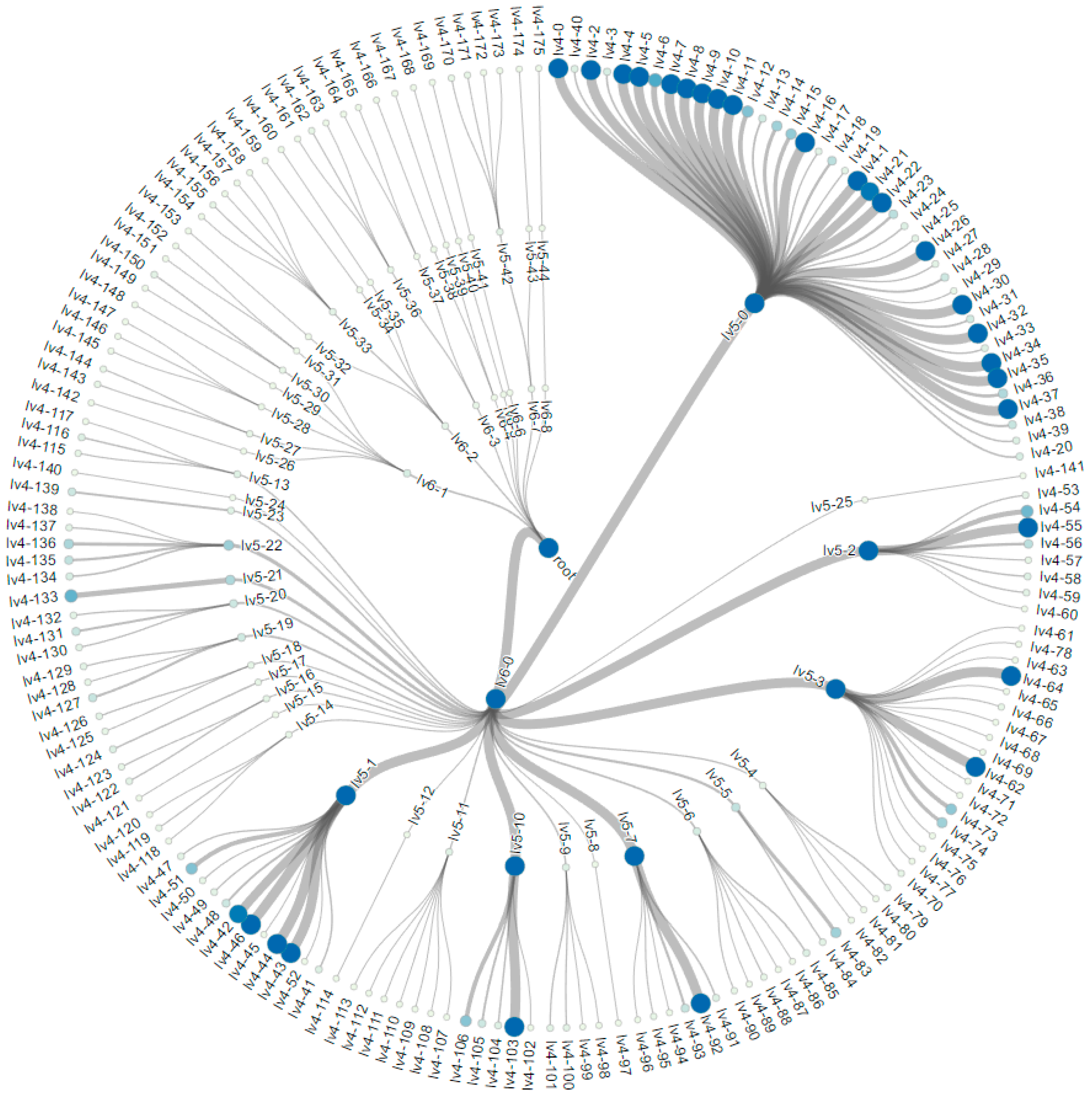
3.2. Construction of the Tree Hierarchy

By running Algorithm 2 with a proper value of t, we can typically generate a redundant number of clusters, each containing a small number of closely positioned data points. If we consider these clusters as the first level of the tree hierarchy, the higher levels of the tree can be built in a bottom-up manner. To build the next level, we see each cluster center as a point in the current level, and then simply run incremental k-means on them with an increased distance threshold. The pseudo code of such an algorithm is given in Algorithm 3.

The height of the tree, as well as its branching factors, are controlled by the initial distance threshold t and the function update_threshold(t), which computes the distance threshold for raising the next level. The initial t can be chosen according to the distribution of the point distances, e.g., the value indicating the average intra-cluster distance of clusters. Then, a practical strategy for updating it could simply be setting up a growth rate so that update_threshold(t) = t * growth rate, i.e., the threshold will grow linearly. However, this can be problematic sometimes, and result in a t’ that is either too large (which merges all points into a single node at an early phase) or too small (which turns each point into a single a cluster in the worst case). Thus, to make it more flexible, we also specify a range of shrinking rate, e.g., from 0.05–0.8, which is the ratio of the number of nodes between the new level and the current level. A threshold t’ is considered ineffective whenever the shrink rate of the new level falls out of the range. In such a case, we predefine the function to compute t’ again in the same manner as the initial t, but based on nodes of the current level. The construction process stops when the current level contains only the root node, or has fewer nodes than a predetermined number. In the latter case, we make the root node with the last level as its children.

Algorithm 3: Incremental K-Means Tree

Input: data points P, initial distance threshold t, batch size s Output: root node of the tree Set each data point in P as a leaf node L = leaves t’ = t while L does not meet the stop condition Perform Alg. 2 with t’ and s to generate C clusters (nodes) from L Make nodes in L as children of the corresponding nodes in C t’ = update_threshold(t) L = C end while if L contains only one node then Return L[0] as the root else Make and return the root with L as its children

3.3. Determine the Distance Threshold

Since Algorithm 2 was merely designed for sampling points in each cluster to downscale the data size [27], the distance threshold $t$ could be specified by the user accordingly to control cluster numbers and sizes. However, as $t$ can directly affect the structure of the result hierarchy in Algorithm 3, it must be assigned carefully.

When looking for a proper value of t for constructing the next level of the tree, we first compute a histogram of the pairwise distances between points in the current level. However, computing the distance matrix could be very compute-intensive, especially given a dataset of high dimensionality. We took two approaches to ease this issue. First, we reduce the number of dimensions by removing the irrelevant ones that have little contribution to the clustering process. As we typically use the Euclidean distance metric, the dimension reduction can be done simply by ignoring dimensions with small standard deviations. Second, when there are too many points, we only use a random sampling of, say, 20,000–50,000 points, instead of all of them, to compute the histogram. The process of computing the distance distribution as well as computing the dimension standard deviations are all GPU-accelerated to further boost the speed. Details of the implementation are given in Section 4.

In our experience, the distribution of point distances in a dataset typically has several peaks and gaps, which indicate internal and external distances between point clusters. A good value of t can then be selected through referencing these values. Although the histogram’s bin width may affect the judgment, we find that the clustering result is not very sensitive to small variations of t. We typically chose 200 bins in our experimentation, while the exact number can be varied for other datasets.

4. Low Level Implementation

The algorithms described in the previous section were implemented on a single NVIDIA GPU with CUDA. We now introduce the GPU kernel implementation in detail.

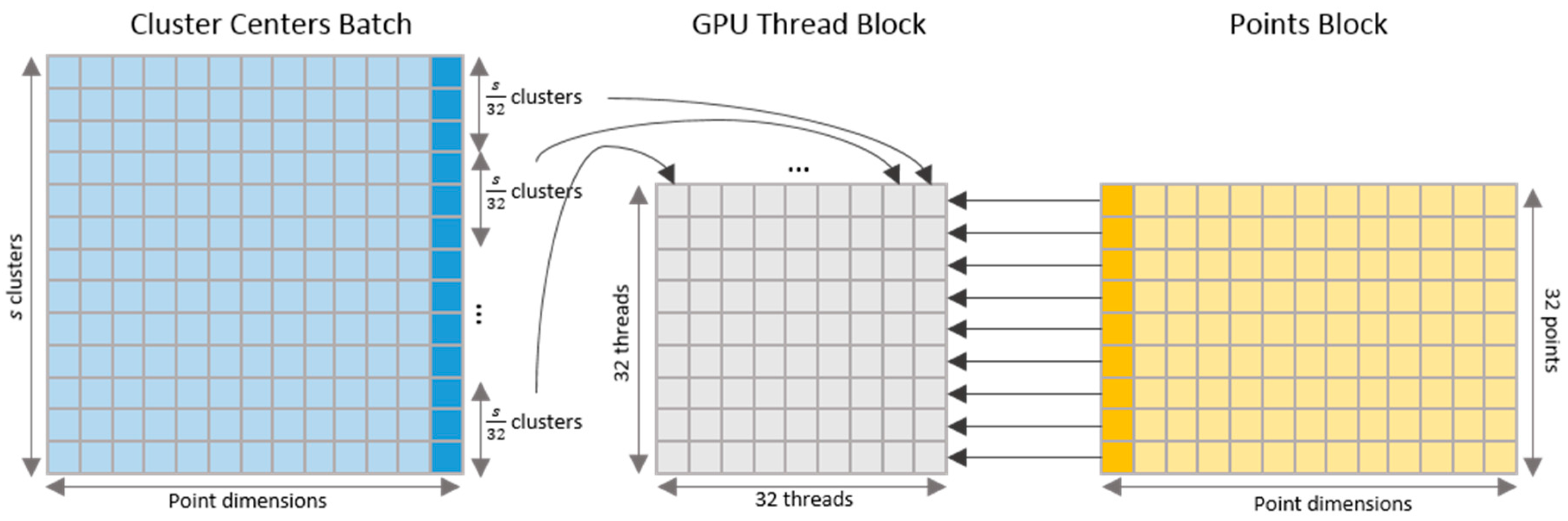
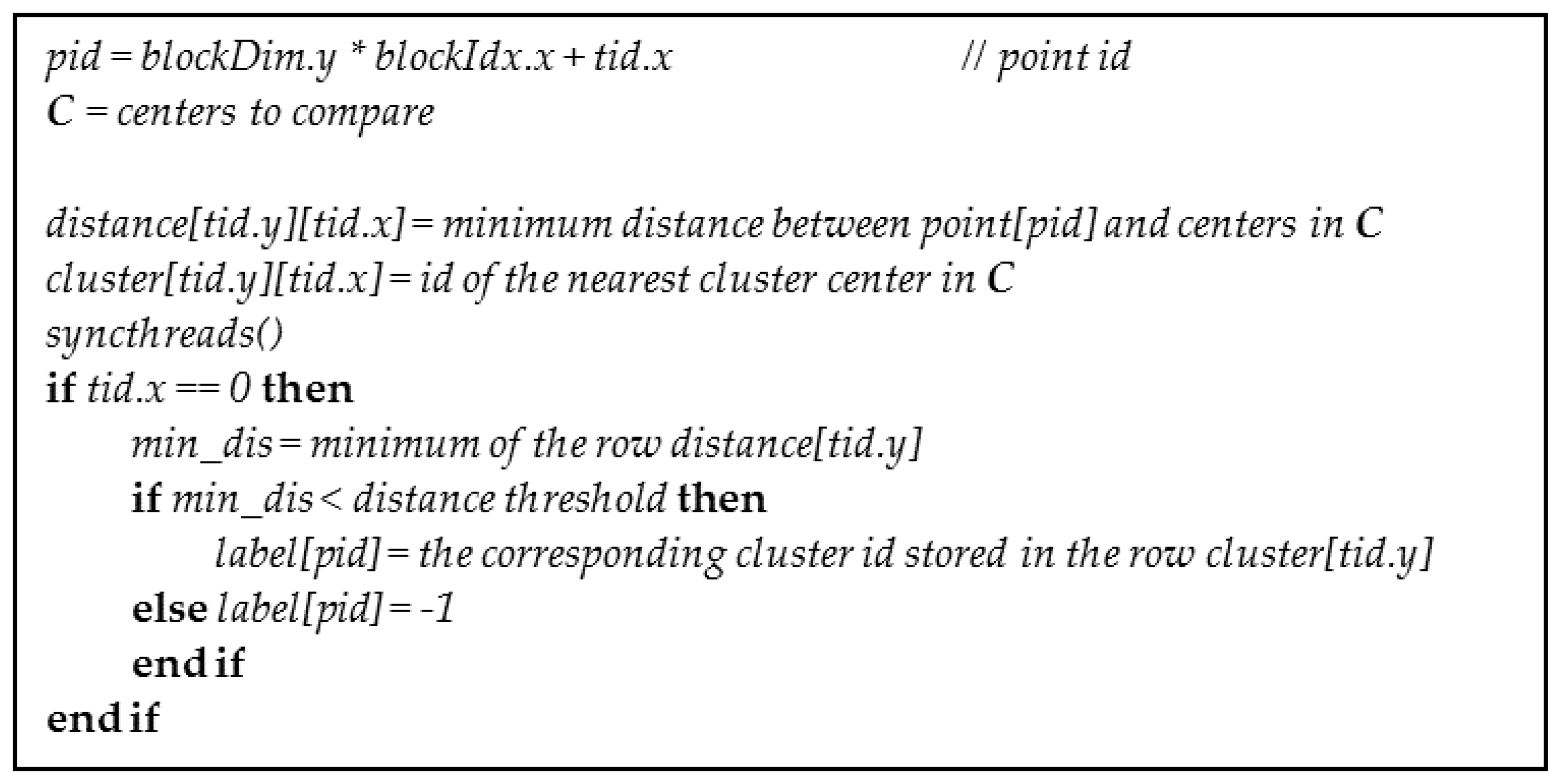
4.1. Kernel for Parallel Clustering

For our parallel incremental k-means, each GPU thread block has a thread dimension of 32 by 32, so that we lunch $N/32$ thread blocks if we have a total of $N$ data points. Figure 1 briefly illustrates the GPU thread block access pattern. Each thread block compares 32 points to a batch of $s$ cluster centers ($s$ must be a multiple of 32). The x coordinate of a thread tells which point it will be operating on, and the y coordinate is mapped to a small group of $s/32$ cluster centers. For example, if we set $s=128$, each thread will process four cluster centers (128/32 = 4). The cluster centers and points are stored in memory as two matrices with the same x dimension. Then, each thread will compute the distances between the corresponding point and the small group of cluster centers, and store the nearest cluster index and its distance value in the shared memory for further processing.

Figure 2 gives the pseudo code for the GPU accelerated algorithm, where the two 32 by 32 shared memories are denoted distance[][] and cluster[][]. Each row of the distance[][] stores the distances between a point and its nearest cluster center in the small group of centers. That is to say, if the batch size is 128, each element of distance[][] stores the distance of the nearest center among the four that are compared against each other in a thread. Meanwhile, the indexes of the corresponding clusters are saved in cluster[][]. Then, after synchronizing all the threads in the block so that all shared memories are filled with stable results, each thread with x id of 0 will scan through one row of the shared memory, looking for the minimum distance and the nearest cluster. A point will be labeled with the nearest cluster’s id if the distance is within the threshold, otherwise the point will be labeled −1, indicating that the point is not clustered in the current iteration of the algorithm (see Algorithm 2). After all the thread blocks finish their job, the labels of all the points will be returned and used for CPU to officially assign points to clusters.

As mentioned, the cluster center batch size s can directly influence the per-thread workload. A larger s means each thread will have to process more cluster centers. The workload of the GPU kernel is also affected by the dimensionality of the data and the computing complexity of the distance metric. Our typical cases are to run the algorithm with datasets of about 400–800 dimensions, and with the Euclidean distance metric. As a result, we found that setting $s=128$ could reach the best workload balance between the GPU and CPU, although the choice for other datasets may vary.

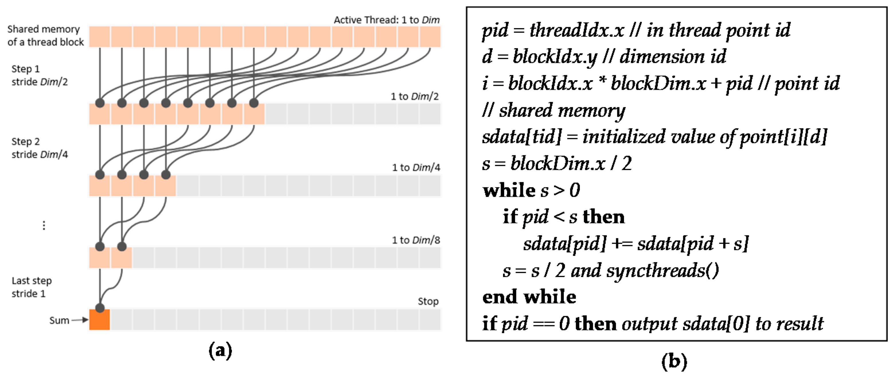
4.2. Parallel Computing of Standard Deviations and Pairwise distances

The computation of the dimension standard deviations is done on the GPU with an optimization technique called parallel reduction [34], which takes a tree-based approach within each GPU thread block. As the data of one dimension forms a very long vector, the calculation of the mean, as well as the standard deviation of the vector, can be transferred into a vector reduction operation (The standard deviation formula is $\sigma =\sqrt{{{\displaystyle \sum }}^{\text{}}{\left(x_i-\mu \right)}^2/N}$, which requires vector mean $\mu$. The part inside the squared root can be transferred into vector summing, which can be done with vector reduction.). For our CUDA implementation, dimensions are mapped to the y-coordinates of blocks. We launch 512 threads in a block, each mapped to the value of one data point in one dimension. Thus, the block dimension is $D$ by $N/512$, where $N$ is the number of points and $D$ is the data dimensionality. The iterative process of the parallel reduction is illustrated in Figure 3a. Each value mapped to a thread is initialized in the beginning. The initialization depends on the goal of the function, i.e., for calculating the vector mean $\mu$, each value is divided by $N$, and for calculating the vector variance, each value $x_i$ is mapped to ${\left(x_i-\mu \right)}^2/N$. And then in each iteration step, the number of active threads in a block is halved, and the values of the second half of the shared memory are added to the first half, until there is only one active thread getting the final result of the block and storing it into the output vector. The pseudo code of the GPU kernel is given in Figure 3b.

The result of the reduction operation is a vector downscaled by 512 times of the input. If the resultant vector is still very large, we can use the parallel reduction again until we reach the final output of a single summed value. However, as the cost of memory transfers may be higher than the benefit from the GPU parallelization when processing a short vector, a single CPU scan would be more than sufficient in such a case. Although it depends on the data volume, at most, two parallel reductions would usually suffice for computing dimension means and standard deviations in our applications.

As we implemented all the algorithms on a single multi-core GPU, a practical difficulty is that there may not be enough GPU memory to hold all the data, especially those of high dimensionality. Even if it is possible to set up a super-large GPU memory, the length of the data array may go beyond the maximum indexable value so that they cannot be accessed. Our solution is to divide data into blocks of the size that can be held in memory of a single GPU, and operate parallel reduction on each of them. Then, an extra CPU scan is operated on results from data blocks to summarize the final output.

The computation of the pairwise distance histogram faces a similar problem. Although we can sometimes fit the sampled data points in GPU memory, the length of the resultant vector can easily go beyond the indexable range (e.g., the length of the vector from pairwise distances of 50,000 points is 1,249,975,000). Then again, we divide sampled points into blocks of fixed size. As we only need the histogram, we update the statistics on the CPU whenever the distances of points from two blocks are returned by the GPU, and then drop the result to save memory. The access pattern of GPU thread blocks for computing pairwise distances is straightforward; each thread calculates one pair of distances. As we use 32 × 32 thread blocks, there will simply be $N/32\times N/32$ blocks launched.

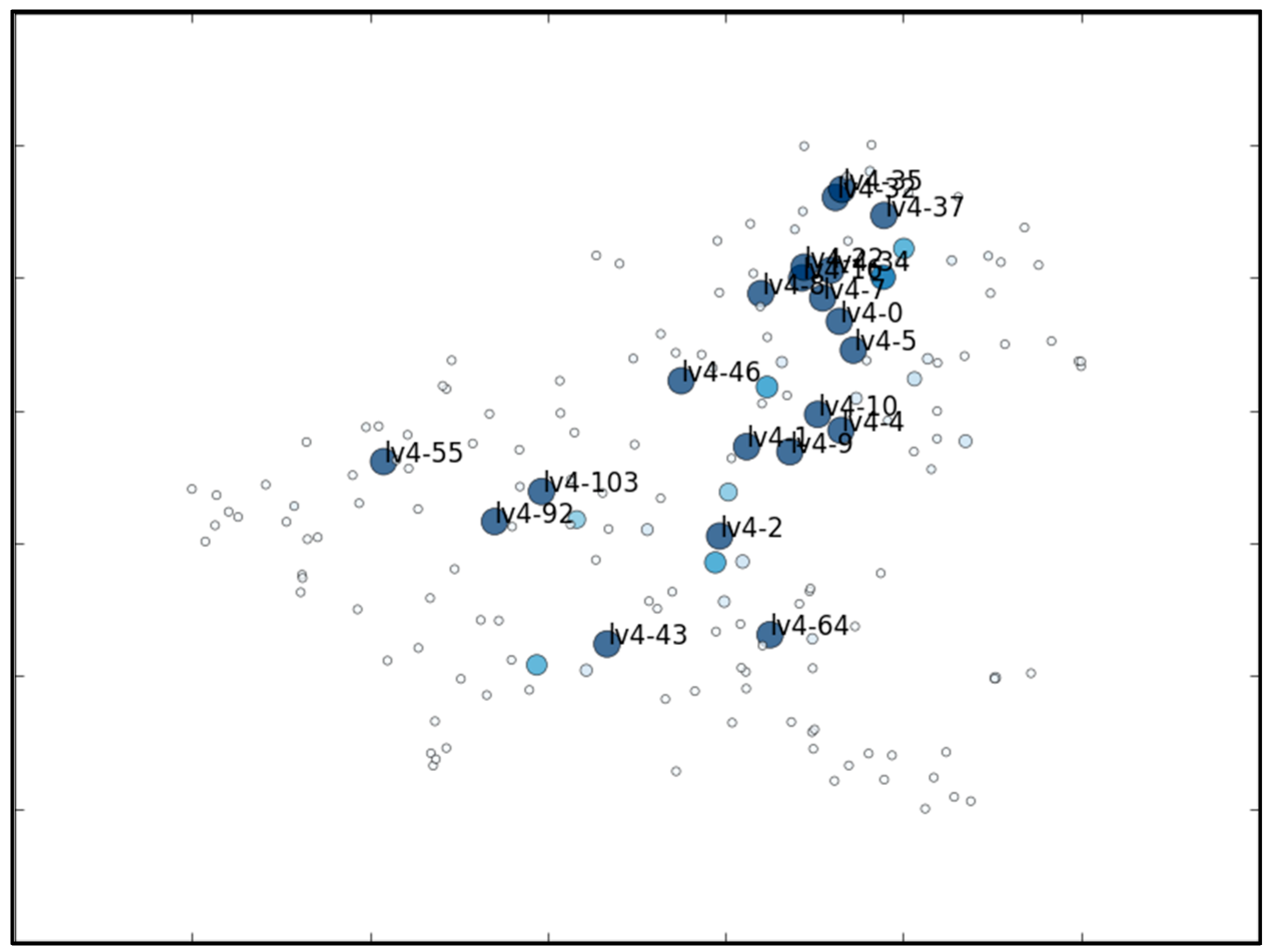
5. Experiments and Visualization

We experimented with two datasets, and in the following, we present our visualizations for communicating the results. For both datasets, we use the Euclidean distance to compare points and cluster centers, based on which data hierarchies are built.

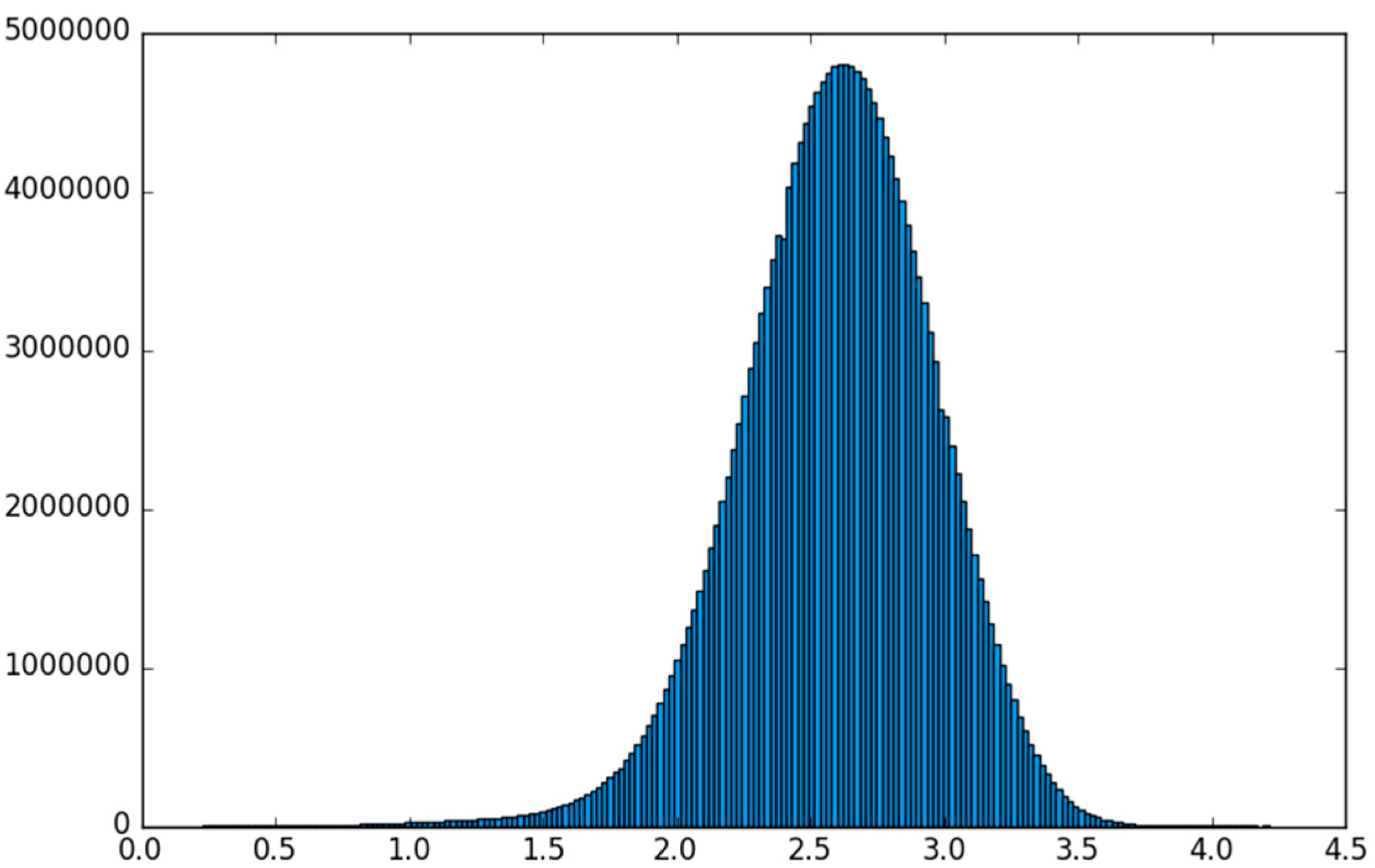
5.1. The MNIST Dataset

The first experiment used the MNIST dataset (http://yann.lecun.com/exdb/mnist/). It contains 55,000 handwritten digit images, each with a resolution of 28 × 28 pixels, i.e., each data point is of 784 dimensions. The greyscale value of a pixel ranges from 0 to 1. As pixels near the edge of an image are usually blank, we filter out these dimensions via the standard deviation scheme, leaving 683 dimensions for use. The histogram of pairwise distances from 20,000 samples is shown in Figure 4. Here, we can see that the histogram generally follows a Gaussian distribution. Considering the multiclass nature of the dataset, the single peak actually implies the range of the interclass distance, and suggests that data points are widespread on the hypersphere.

Referencing Figure 4, we decide to build the tree with an initial distance threshold of 1.4 and a distance growth rate of 1.1. Such a small initial threshold means that the first level of the tree mainly serves for data downscaling. We can then construct a tree hierarchy with a total of seven levels by running our parallel algorithm. The distance thresholds used, and the number of nodes that built each level of the tree are both listed in

Table 1. Distance thresholds and the number of nodes for each tree level of the MNIST dataset.

Level	1	2	3	4	5	7	8 (root)
Distance threshold	1.4	1.54	1.70	1.86	2.05	2.25	2.48
Number of nodes	20,610	2928	521	205	83	19	1

.

As upper levels of the tree usually contain more meaningful knowledge, we cut the tree at level three to generate the final output. We then visualize the result with the extended circular dendrogram, as illustrated in Figure 5. Here, only significant nodes with more than five data points are rendered. In the dendrogram, the root node is located in the center, and nodes on levels farther from the root are located in outer circles. A node is named after its level and its ID on the level. The size and the color of a node signify the number of data points it contains, decided by the formula

$$\mathrm{s}=\theta \left(n/l\right),$$

(1)

where $n$ is the number of member points, $l$ is the level of the node, and $\theta \left(·\right)$ scales and regulates the range of the output. We use a color map from white to blue regarding the RGB value. This means that a larger node with a bluer color owns more member points than a node on the same level of the dendrogram, but with a smaller size and a lighter color. Nodes between two neighboring levels are connected with edges. The width of an edge indicates the amount of point merged from a child node to its parent node, where a wide edge from the parent node connects a child of large number of members. By such, dominant branches of the tree can be easily recognized.

There are some interesting structures we can observe in Figure 5. First, node lv4-0 is a very big node, which absorbs most level-three nodes, including a few large ones. This could mean that many clusters generated on level three have already been very similar to each other. However, there are other nodes, e.g., lv3-434, going up to the root via other branches. To have a deeper investigation, we look at the images included in the different nodes. Then, we find that even though lv3-434 and lv3-3 are all nodes containing images of digit 0, the images in lv3-3 (Figure 6b) are much more skewed than those in lv3-434 (Figure 6a), so that they are nearer to images of other nodes merged into lv4-0, e.g., node lv3-7 (Figure 6c), regarding the Euclidean distance.

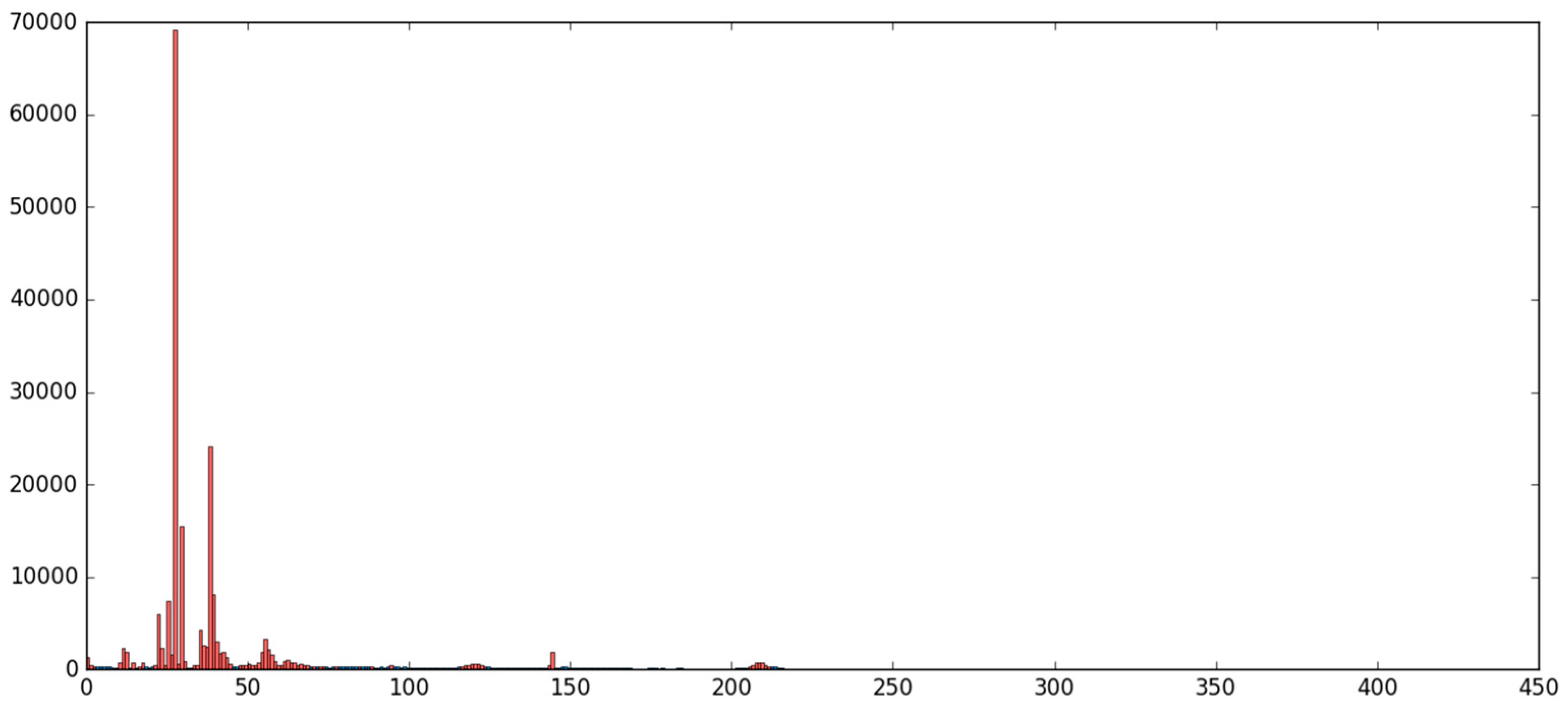
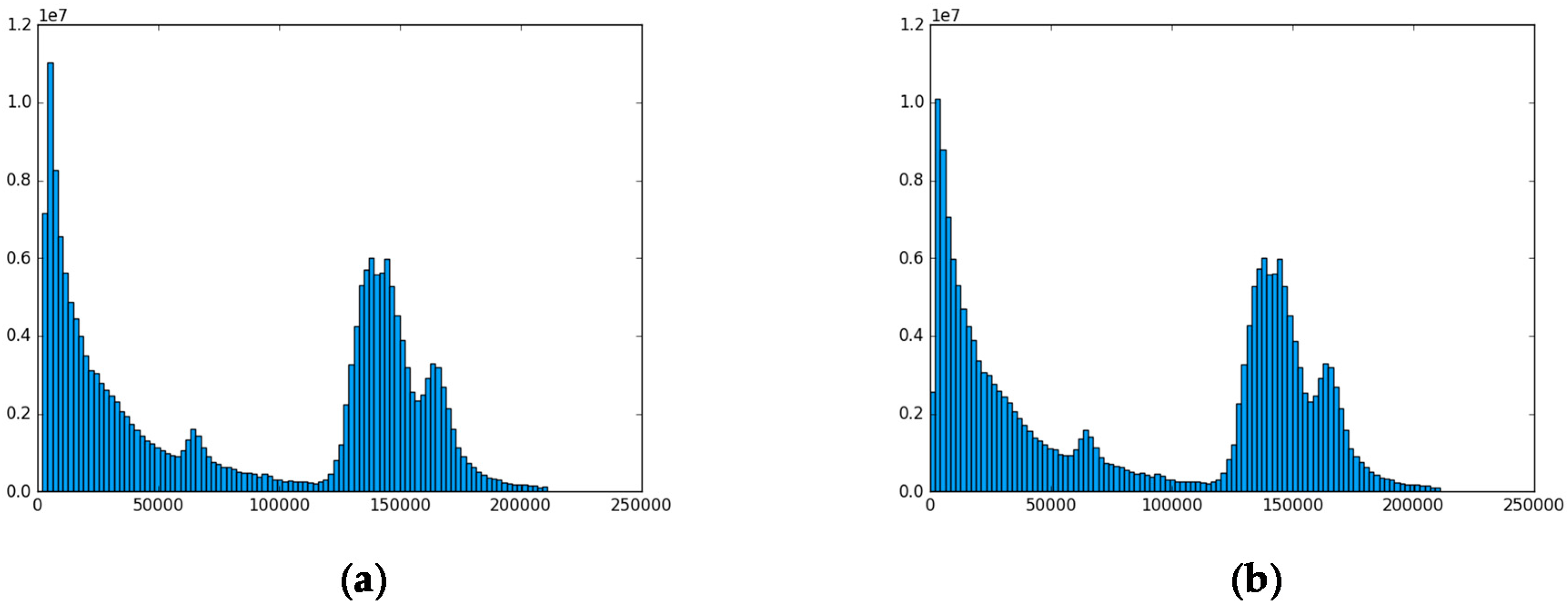
5.2. The Aerosol Dataset

The Aerosol dataset was collected for atmospheric chemistry to understand the processes that control the atmospheric aerosol life cycle. The dataset was acquired by a state-of-the-art single particle mass spectrometer, termed SPLAT II (see [35] for more detail). Each data point in the dataset is a 450-dimensional mass spectra of an individual aerosol particle. The dataset we use contains about 2.7 million data points. The standard deviation of each dimension is shown in Figure 7, where we can observe that a few dimensions are apparently more variant than others. By setting a threshold of 0.01 of the max standard deviation, 36 dimensions are selected and marked with red bars in Figure 7, while the remaining bars are colored blue (most of which are too small to be observed clearly). We sampled 20,000 points to compute the distance histogram. Here, we demonstrate two histograms respectively calculated with all 450 dimensions (Figure 8a), and only the 36 dimensions (Figure 8b). The two histograms are almost identical, implying that the reduction of dimension will not affect the result.

The histograms in Figure 8 clearly shows several peaks, where the leftmost peak indicates the intraclass distance of most clusters, and the rest imply interclass distances. Hence, we set the initial distance threshold t = 5000, which is the leftmost peak’s distance value, so that these small dense clusters can be recognized. Since the volume of the dataset is quite large, we set the growth rate of the distance threshold to be 2.0, i.e., the distance threshold will be doubled whenever building the next level of the hierarchy. In this way, the distance threshold can quickly grow such that there are fewer nodes with a large branching factor in each level, and hence, the result tree structure may have a controllable height.

The distance thresholds for constructing each level of the tree, as well as the resultant number of nodes in each level, are given in

Table 2. Distance thresholds and the resulted number of nodes for each level of the Aerosol dataset.

Level	1	2	3	4	5	6	7 (root)
Distance threshold	5 k	10 k	20 k	40 k	80 k	160 k	320 k
Number of nodes	196,591	4549	709	176	45	9	1

. Although the dataset is large, the resulted hierarchy has only seven levels in total. Due to the fast growth of the distance threshold, the number of nodes shrinks rapidly between levels. Given the background knowledge that there are actually about 20 types of particles in the dataset, we cut the tree at level four. This also makes the visualization more manageable. We visualize the final result again with the extended circular dendrogram in Figure 9.

From Figure 9, we can see that while node lv6-0 is the dominating child for the root, it has a few large sub-branches (referencing the thick edge to lv6-0 from lv5-0, lv5-1, lv5-10, lv5-3, etc.). Also by observing that all other nodes on level six are comparably very small (with small node sizes and thin edges), some good clustering of different particles may have been recognized on level five. However, it seems that some level-five nodes (e.g., lv5-0 and lv5-1) are still too inclusive and variant, as they own some thick branches and many of their children are also big nodes. This implies that some clusters are mixed due to their closely located centers.

Figure 10 demonstrates the t-SNE layout [33] of all level-four nodes. The point sizes and colors (from white to blue) in the scatter plot are scaled regarding the nodes’ number of members. Some of the largest nodes are labeled. In Figure 10, we see that children of the node lv5-0 are all closely located, while other nodes (e.g., lv4-43, child of lv5-1, and lv4-55, child of lv5-2) are farther away. This confirms the correctness of the tree structure. Among children of lv5-0, there are seemingly two sub-clusters: one around lv4-0, and one around lv4-10. This could imply different types of particles.

A further analysis may reveal more knowledge of the dataset, but doing so would go beyond the focus and scope of this paper. However, the presented examples have sufficiently demonstrated the validity of our algorithm, as well as the effectiveness of the visualization.

6. Discussion and Conclusions

We have presented the algorithm of incremental k-means tree for big data management, as well as its GPU-accelerated construction and visualization. Its effectiveness has been demonstrated by experimenting on two real-world datasets. Nevertheless, there are a few issues worth discussion.

First, we have not conducted experiments testing the exact timings of our algorithm under different scales of data volume. Although this could be a potential future work, the actual time cost is also related to the settings of the initial distance threshold and its growth. For constructing each level, a large distance threshold not only means a smaller number of clusters to be learned, but also more points will be clustered in one scan of data, and hence, fewer iterations and shorter running time. In addition, the number of nodes for building the next level of the hierarchy will be better downscaled, making the rest of the hierarchy construction even faster. As a reference, for the two datasets and their specific settings used in this paper, building the hierarchy from the MNIST dataset cost about four and half minutes, and from the Aerosol dataset about 30 min.

Although the resultant hierarchy is decided by the algorithm parameters and the distance metric employed, the stability of the result under different settings depends on the dataset. We have seen in the MNIST dataset example that the distance threshold changes between levels are quite small, yet the number of nodes is fast narrowing as levels grow. This means that this dataset could be very sensitive to parameter settings, so that a small variation could lead to big changes in the result structure. In contrast, we also tested on the Aerosol dataset, with some initial distance thresholds a few hundred off from 5000. However, the results are basically the same as shown in Section 5.2, with only small differences on the number of nodes in each level.

Also, our algorithm can be applied to datasets from a wide range of areas, and the result hierarchy can be used in any further analysis requires such information. For example, we can conduct a fast nearest search or hierarchical sampling on the MNIST dataset with the constructed structure, and clustering on the Aerosol dataset. Acquiring such structural information is often a general and important step in big data pre-processing.

Finally, the extended circular dendrogram presented in this paper could be further developed. A richer scope of information, such as the quality metric of each node for instance, could be visualized to make the graph more informative. Interactions can also be added so that users can visually explore and modify the hierarchy to look for new knowledge from data. Based on these developments, a comprehensive visual analytic interface could be well established. This is the subject of future work.

References

1. Big data. Nature 2008, 455, 1–136.
2. Dealing with data. Science 2011, 331, 639–806.
3. Muja, M.; Lowe, D.G. Scalable nearest neighbor algorithms for high dimensional data. IEEE Trans. Pattern Anal. Mach. Intell. 2014, 36, 2227–2240. [Google Scholar] [CrossRef] [PubMed]
4. Dasgupta, S.; Hsu, D. Hierarchical sampling for active learning. In Proceedings of the 25th International Conference on Machine Learning, Helsinki, Finland, 5–9 July 2008; pp. 208–215. [Google Scholar]
5. Fahad, A.; Alshatri, N.; Tari, Z.; Alamri, A.; Khalil, I.; Zomaya, A.Y.; Foufou, S.; Bouras, A. A survey of clustering algorithms for big data: Taxonomy and empirical analysis. IEEE Trans. Emerg. Top. Comput. 2014, 2, 267–279. [Google Scholar] [CrossRef]
6. Wong, P.C.; Shen, H.W.; Johnson, C.R.; Chen, C.; Ross, R.B. The top 10 challenges in extreme-scale visual analytics. IEEE Comput. Graph. Appl. 2012, 32, 63–67. [Google Scholar] [CrossRef] [PubMed]
7. MacQueen, J. Some methods for classification and analysis of multivariate observations. In Proceedings of the Fifth Berkeley Symposium on Mathematical Statistics and Probability, Berkeley, CA, USA, 21 June–18 July 1965 and 27 December 1965–7 January 1966; Lucien, C., Jerzy, N., Eds.; University of California Press: Berkeley, CA, USA, 1967; Volume 1, pp. 281–297. [Google Scholar]
8. Farivar, R.; Rebolledo, D.; Chan, E. A parallel implementation of k-means clustering on GPUs. In Proceedings of the International Conference on Parallel and Distributed Processing Techniques and Applications, PDPTA 2008, Las Vegas, NV, USA, 14–17 July 2008; Volume 13, pp. 340–345. [Google Scholar]
9. Bezdek, J. C.; Ehrlich, R.; Full, W. FCM: The fuzzy c-means clustering algorithm. Comput. Geosci. 1984, 10, 191–203. [Google Scholar] [CrossRef]
10. Zhang, T.; Ramakrishnan, R.; Livny, M. BIRCH: An Efficient Data Clustering Method for Very Large Databases; ACM: New York, NY, USA, 1996; Volume 25, pp. 103–114. [Google Scholar]
11. Guha, S.; Rastogi, R.; Shim, K. CURE: An efficient clustering algorithm for large databases. Inf. Syst. 2001, 26, 35–58. [Google Scholar] [CrossRef]
12. Karypis, G.; Han, E.H.; Kumar, V. Chameleon: hierarchical clustering using dynamic modeling. Computer 1999, 32, 68–75. [Google Scholar] [CrossRef]
13. Ester, M.; Kriegel, H.P.; Sander, J.; Xu, X. A Density-Based Algorithm for Discovering Clusters in Large Spatial Databases with Noise. In Proceedings of the International Conference on Knowledge Discovery and Data Mining, Portland, OR, USA, 2–4 August 1996; pp. 226–231. [Google Scholar]
14. Ankerst, M.; Breunig, M.M.; Kriegel, H.; Sander, J. OPTICS: Ordering Points to Identify the Clustering Structure; ACM: New York, NY, USA, 1999; Volume 28, pp. 49–60. [Google Scholar]
15. Agrawal, R.; Gehrke, J.; Gunopulos, D.; Raghavan, P. Automatic Subspace Clustering of High Dimensional Data for Data Mining Applications; ACM: New York, NY, USA, 1998; Volume 27, pp. 94–105. [Google Scholar]
16. Wang, W.; Yang, J.; Muntz, R. STING: A statistical information grid approach to spatial data mining. Int. Conf. Very Large Data 1997, 97, 1–18. [Google Scholar]
17. Fraley, C.; Raftery, A.E. MCLUST: Software for Model-Based Cluster Analysis. J. Classif. 1999, 16, 297–306. [Google Scholar] [CrossRef]
18. Dempster, A.P.; Laird, N.M.; Rubin, D.B. Maximum Likelihood from Incomplete Data via the EM Algorithm. J. R. Stat. Soc. Ser. B 1977, 39, 1–38. [Google Scholar]
19. Bentley, J.L. Multidimensional binary search trees used for associative searching. Commun. ACM 1975, 18, 509–517. [Google Scholar] [CrossRef]
20. Freidman, J.H.; Bentley, J.L.; Finkel, R.A. An Algorithm for Finding Best Matches in Logarithmic Expected Time. ACM Trans. Math. Softw. 1977, 3, 209–226. [Google Scholar] [CrossRef]
21. Silpa-Anan, C.; Hartley, R. Optimised KD-trees for fast image descriptor matching. In Proceedings of the IEEE Conference on Computer Vision and Pattern Recognition, Anchorage, AK, USA, 23–28 June 2008; pp. 1–8. [Google Scholar]
22. Lamrous, S.; Taileb, M. Divisive Hierarchical K-Means. In Proceedings of the International Conference on Computational Inteligence for Modelling Control and Automation and International Conference on Intelligent Agents Web Technologies and International Commerce, Sydney, Australia, 28 November–1 December 2006. [Google Scholar]
23. Jose Antonio, M.H.; Montero, J.; Yanez, J.; Gomez, D. A divisive hierarchical k-means based algorithm for image segmentation. In Proceedings of the IEEE International Conference on Intelligent Systems and Knowledge Engineering, Hangzhou, China, 15–16 November 2010; pp. 300–304. [Google Scholar]
24. Nister, D.; Stewenius, H. Scalable Recognition with a Vocabulary Tree. In Proceedings of the IEEE Computer Society Conference on Computer Vision and Pattern Recognition, New York, NY, USA, 17–22 June 2006; Volume 2, pp. 2161–2168. [Google Scholar]
25. Imrich, P.; Mueller, K.; Mugno, R.; Imre, D.; Zelenyuk, A.; Zhu, W. Interactive Poster: Visual data mining with the interactive dendrogram. In Proceedings of the IEEE Information Visualization Symposium, Boston, MA, USA, 28–29 October 2002. [Google Scholar]
26. Satish, N.; Harris, M.; Garland, M. Designing efficient sorting algorithms for manycore gpus. In Proceedings of the IEEE International Parallel and Distributed Processing Symposium, Rome, Italy, 23–29 May 2009. [Google Scholar]
27. Papenhausen, E.; Wang, B.; Ha, S.; Zelenyuk, A.; Imre, D.; Mueller, K. GPU-accelerated incremental correlation clustering of large data with visual feedback. In Proceedings of the IEEE International Conference on Big Data, Silicon Valley, CA, USA, 6–9 October 2013; pp. 63–70. [Google Scholar]
28. Herrero-lopez, S.; Williams, J.R.; Sanchez, A. Parallel Multiclass Classification Using SVMs on GPUs. In Proceedings of the 3rd Workshop on General-Purpose Computation on Graphics Processing Units, Pittsburgh, PA, USA, 14 March 2010; ACM: New York, NY, USA, 2010; p. 2. [Google Scholar]
29. Liang, S.; Liu, Y.; Wang, C.; Jian, L. A CUDA-based parallel implementation of K-nearest neighbor algorithm. In Proceedings of the International Conference on Cyber-Enabled Distributed Computing and Knowledge Discovery, Zhangjiajie, China, 10–11 October 2009; pp. 291–296. [Google Scholar]
30. Jia, Y.; Shelhamer, E.; Donahue, J.; Karayev, S.; Long, J.; Girshick, R.; Guadarrama, S.; Darrell, T. Caffe: Convolutional architecture for fast feature embedding. In Proceedings of the 22nd ACM International Conference on Multimedia, Orlando, FL, USA, 3–7 November 2014; ACM: New York, NY, USA, 2014; pp. 675–678. [Google Scholar]
31. Kreuseler, M.; Schumann, H. A flexible approach for visual data mining. IEEE Trans. Vis. Comput. Graph. 2002, 8, 39–51. [Google Scholar] [CrossRef]
32. Beham, M.; Herzner, W.; Groller, M.E.; Kehrer, J. Cupid: Cluster-Based Exploration of Geometry Generators with Parallel Coordinates and Radial Trees. IEEE Trans. Vis. Comput. Graph. 2014, 20, 1693–1702. [Google Scholar] [CrossRef] [PubMed]
33. Van Der Maaten, L.J.P.; Hinton, G.E. Visualizing high-dimensional data using t-sne. J. Mach. Learn. Res. 2008, 9, 2579–2605. [Google Scholar]
34. Harris, M. Optimizing Parallel Reduction in CUDA. In NVIDIA CUDA SDK 2. 2008; NVIDIA Developer: Santa Clara, CA, USA, August 2008. [Google Scholar]
35. Zelenyuk, A.; Yang, J.; Choi, E.; Imre, D. SPLAT II: An Aircraft Compatible, Ultra-Sensitive, High Precision Instrument for In-Situ Characterization of the Size and Composition of Fine and Ultrafine Particles. Aerosol Sci. Technol. 2009, 43, 411–424. [Google Scholar] [CrossRef]
Figure 1. GPU access pattern for the parallel clustering algorithm.
Informatics 04 00024 g001
Figure 2. The pseudo code of GPU kernel for parallel clustering.
Informatics 04 00024 g002
Figure 3. The parallel reduction. (a) Illustration of GPU thread block iterations. (b) The pseudo code of the GPU kernel implementation.
Informatics 04 00024 g003
Figure 4. Distribution of sampled points’ pairwise distances from the MNIST dataset.
Informatics 04 00024 g004
Figure 5. The extended circular dendrogram visualizing the hierarchy built from the MNIST dataset.
Informatics 04 00024 g005
Figure 6. Images contained in different level three nodes. (a) An image of digit 0 from node lv3-434. (b) An image of digit 0 from node lv3-3. (c) An image of digit 8 from lv3-7. Considering the Euclidean distance, (b) and (c) could be closer than (a) and (b).
Informatics 04 00024 g006
Figure 7. Standard deviations of each dimension of the Aerosol dataset. By applying a threshold of 0.01 of the max standard deviation, only 36 dimensions are selected for use.
Informatics 04 00024 g007
Figure 8. The distribution of point distances in the Aerosol dataset. (a) The histogram calculated with all 450 dimensions. (b) The histogram calculated with the selected 36 dimensions. The two are almost identical, implying that dimension reduction will not affect the result.
Informatics 04 00024 g008
Figure 9. The extended circular dendrogram visualizing the hierarchy constructed from the Aerosol dataset.
Informatics 04 00024 g009
Figure 10. The t-SNE layout of nodes on level four.
Informatics 04 00024 g010