
Sampling and Estimation of Pairwise Similarity in Spatio-Temporal Data Based on Neural Networks

Abstract
1. Introduction
2. Related Work
2.1. Visualization of Spatio-Temporal Data
2.2. Similarity Matrices to Directly Visualize and Analyze Similarity Information
2.3. Machine Learning for Image Interpolation and Similarity Learning
3. Overview
3.1. Similarity Information from Spatio-Temporal Data
3.2. Neural Networks Basics (for Time Series Similarity Estimation)
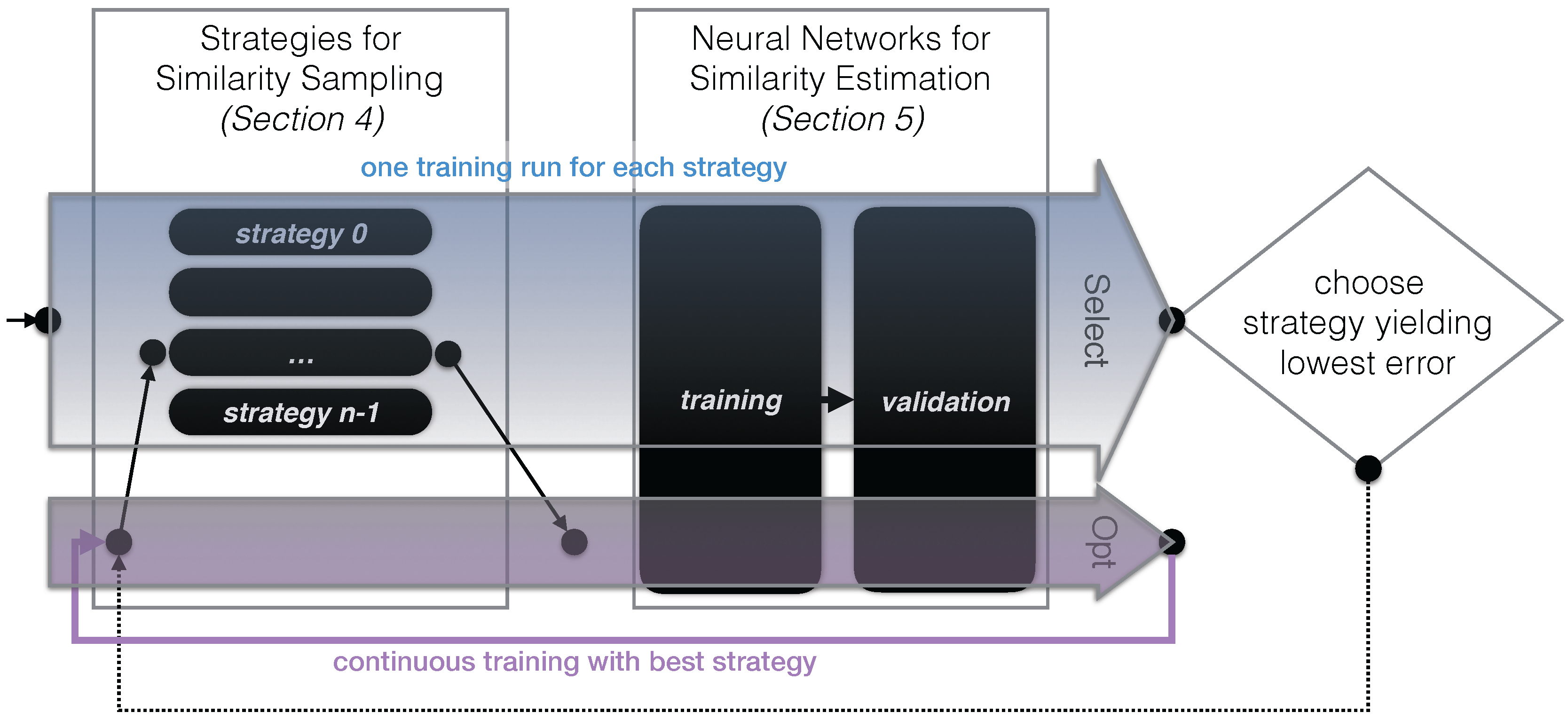
3.3. Approach Outline
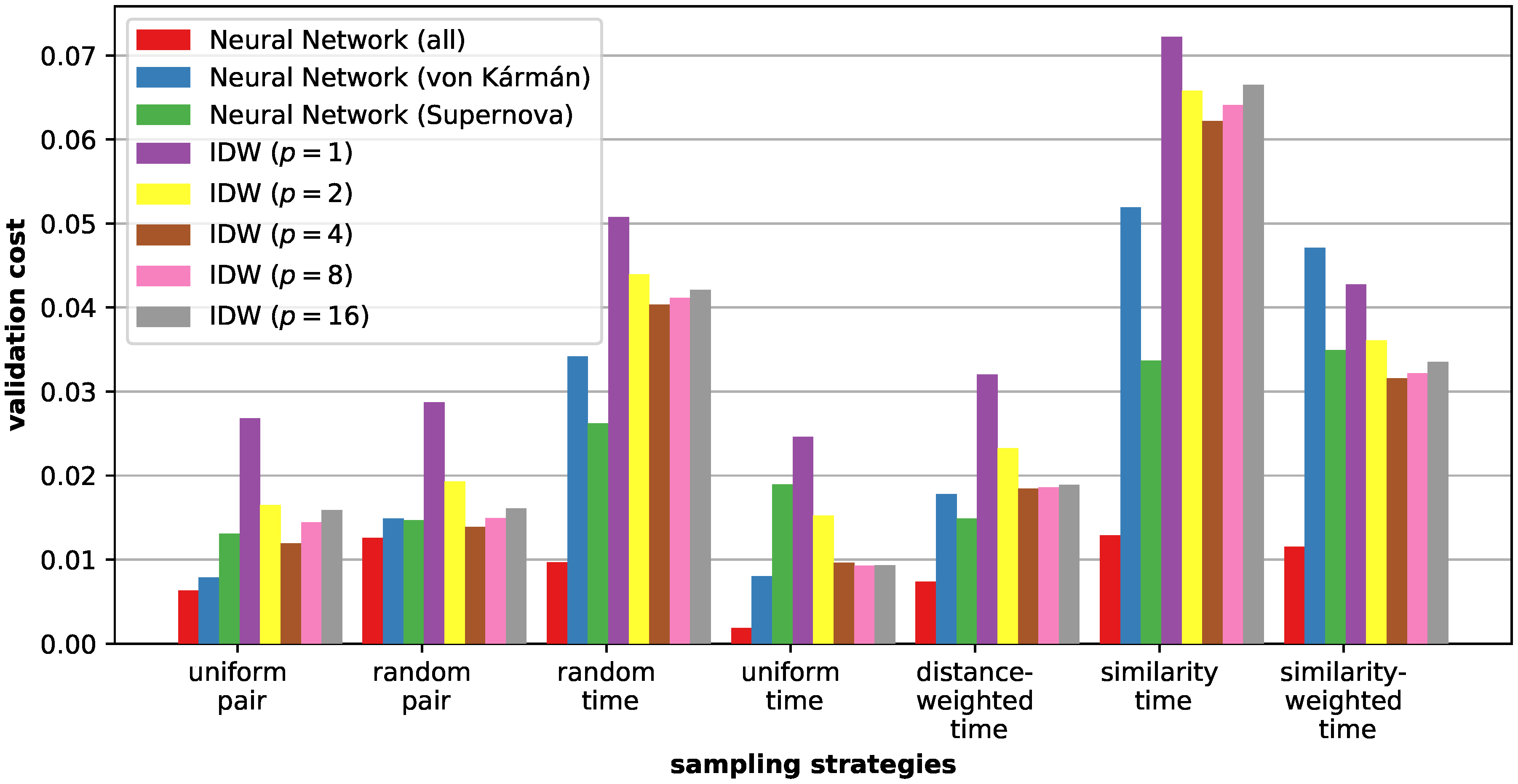
4. Strategies for Similarity Sampling
- (1)
- uniform pair. In this strategy, the goal is to distribute samples in the temporal space as evenly as possible (in a progressive fashion). Doing this, we start out with a random sample pair and . Subsequently, we then iteratively compute the new similarity pair that has the maximum distance to any of the pairs (i.e., to any of the pairs that have been computed so far).
- (2)
- random pair. A time step pair—that has not been computed yet —is chosen randomly and processed next.
- (3)
- random time. A random time step is selected that has not yet been considered (). As described above, before adding a new time step, first all pairwise combinations of time steps are computed before proceeding further.
- (4)
- uniform time. Select the time step in between the largest interval range in (with and denoting subsequent time steps ). In case there are multiple intervals with the same size, we choose one randomly.
- (5)
- distance-weighted time. Choose a time step randomly (similar to (3)), but the probability of selecting an interval is weighted by (akin to the selection criterion in (4)).
- (6)
- similarity time. Consider the distance between two subsequent time steps in T: . Add a time step in the interval with the largest distance.
- (7)
- similarity-weighted time. Select an interval randomly to add a new time step to , with the probability being weighted by .
5. Neural Networks for Similarity Estimation
5.1. Model Setup
- 1.
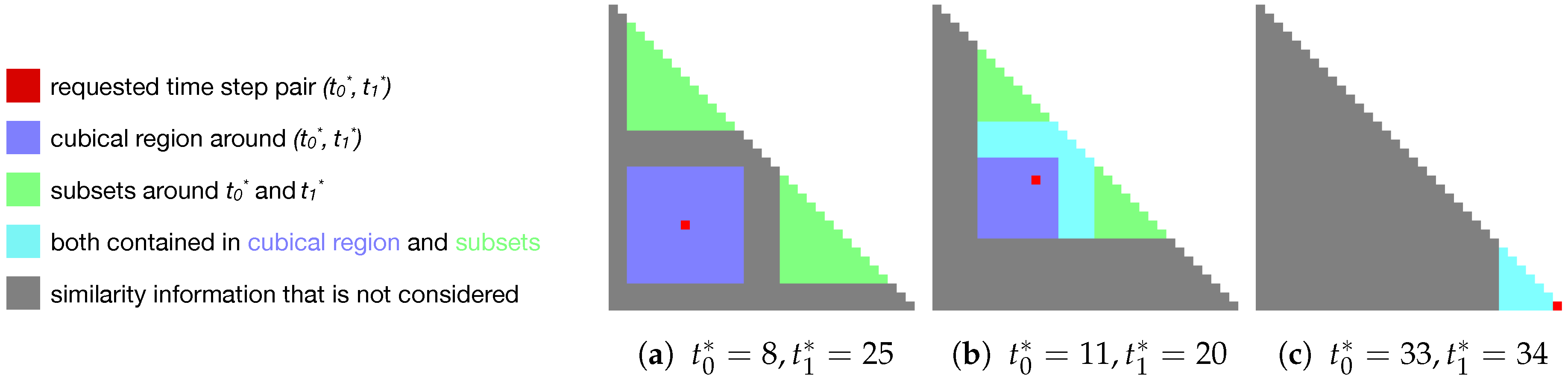
- The cubical region around , except for itself (blue in Figure 5):This results in elements. This gives the similarity of close pairs in temporal space.
- 2.
- Two subsets of the similarity matrix, one around and one around (i.e., containing all pairwise combinations of time steps and , respectively) (green in Figure 5). This results in a total of (according to Equation (1)), and gives the similarity to close time steps for each component of the pair.
5.2. Training and Validation Data Preparation
| Algorithm 1 Generation of similarity data sets (for training, validation, and testing) |
|
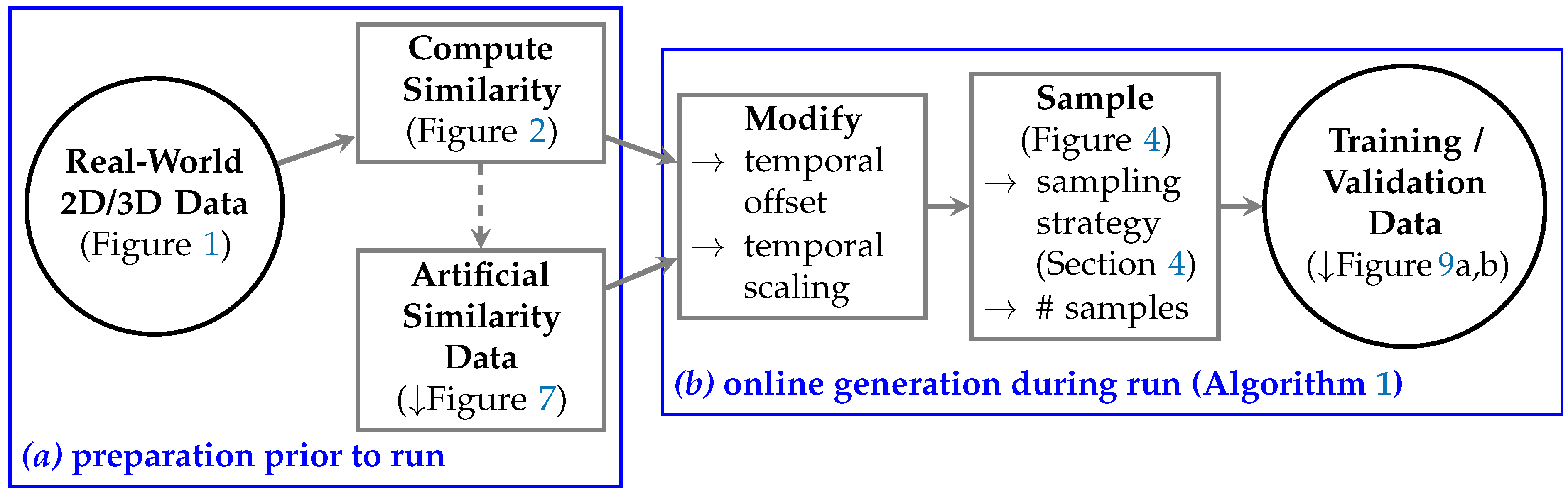
- Real–World 2D/3D Data.
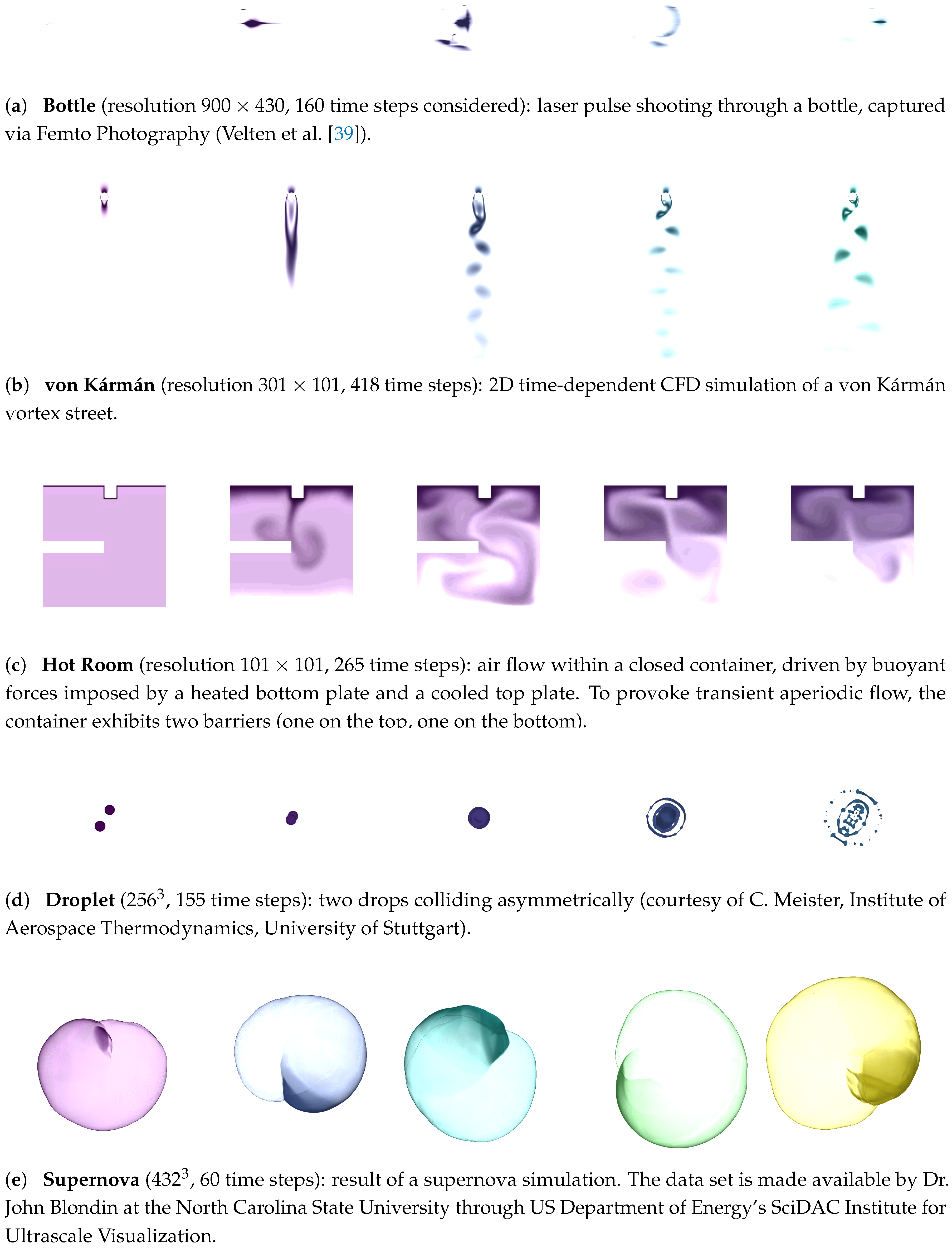
- As input, we use a set of typical real-world 2D/3D + time data sets (Figure 1).
- Compute Similarity.
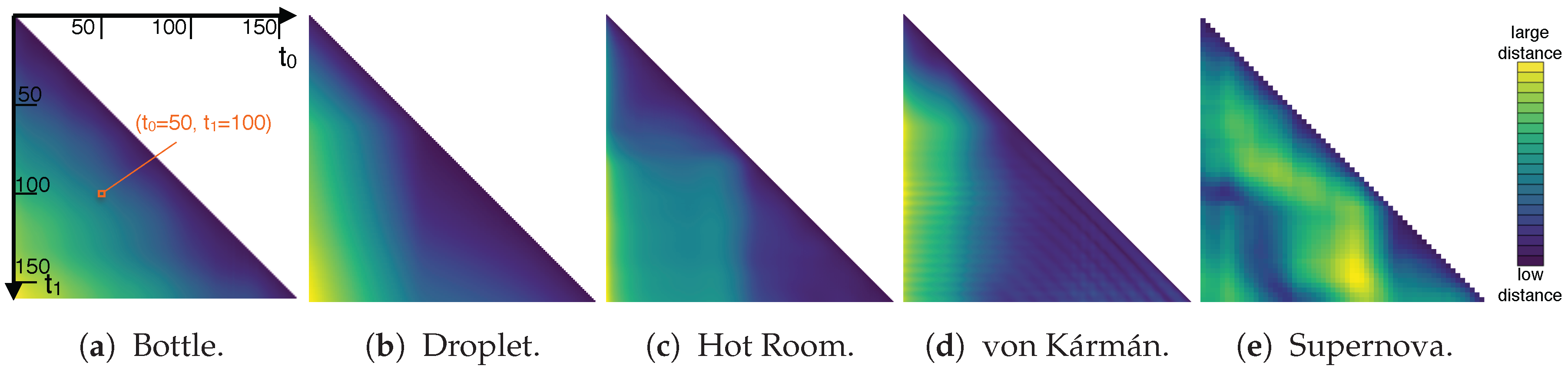
- To compute the pairwise distances between different time steps within each series, we use the approach proposed by Frey and Ertl [24,25]. It is used to make it computationally feasible to directly compute the similarity between high-resolution field data sets. Conceptually, it starts with an initial random assignment of so-called source elements from one data set to so-called target elements of the other data set (each element refers to a (scalar) mass unit given at a certain cell/position in the data). Then, this assignment is improved iteratively in the following. In each iteration, source elements exchange respectively assigned target elements under the condition that this improves the assignment. For this, the quality of an assignment is quantified by d, that essentially computes the sum of weighted distances of the assignments. Here, assignments are weighted by the scalar quantity that is transported. We use this value d directly (on the basis of Euclidean distances) to quantify the distance between the respective time steps. The respective results are shown in Figure 2. Please refer to Frey and Ertl [24,25] for a more detailed discussion.
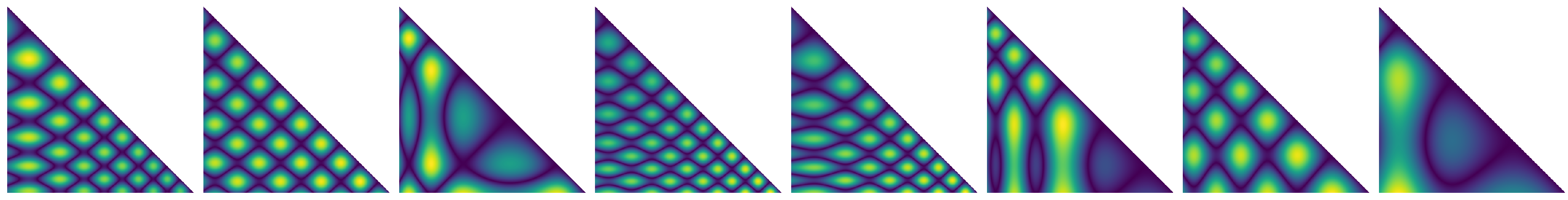
- Artificial Similarity Data.
- Only using a small number of data sets is not sufficient to cover the large variety of typical patterns of similarity information in general, and might also be dangerous in terms of training the network regarding the concrete data rather than generalizing for similarity estimation. Therefore, we added further, synthetically-generated time series data to supplement this. Here, the idea is to mimic the typical patterns that we have seen occurring in the similarity data, yet providing a larger variety to yield better generalization characteristics after learning. For this, we used the following equation for , and three random values :We then compute similarity information from these, and use it during training and validation (Figure 7).
- Modify.
- We do not use the obtained similarity information directly, but randomly offset and scale the time series to get numerous variations on the basis of the available data. We outline our approach to prepare the training data X by means of Algorithm 1 (validation data is generated accordingly). We randomly pick data sets from our collection of real-world and artificial data (Line 10). To modify the data, we randomly choose a scaling factor s, that basically defines the step size with which time steps are considered (Line 12). Then, we use a random offset, which basically determines the first time step that is considered in a time series (Line 14). Finally, we employ this information to generate a new training element (Lines 16–19), each one consisting of time steps (we use throughout this work).
- Sample.
- We then take a random number of samples s from the modified similarity data using the respective sampling strategy (cf. discussion in Figure 4, Line 21).
- Training / Validation Data.
- Finally, this yields the data that can be used for training and validation of the neural network. In more detail, each training / validation data element consists of a pair: (1) the original similarity data after Modify, and (2) the respective data after Sample. Each (1) and (2) contains pairwise similarity information between time steps (a portion of this information has been removed from (2)).
5.3. Similarity Estimation
| Algorithm 2 Our approach to estimate missing similarity information based on neural networks (see Figure 3 for a conceptual overview). |
|
6. Results
6.1. Evaluation Setup
6.2. Sampling Strategies
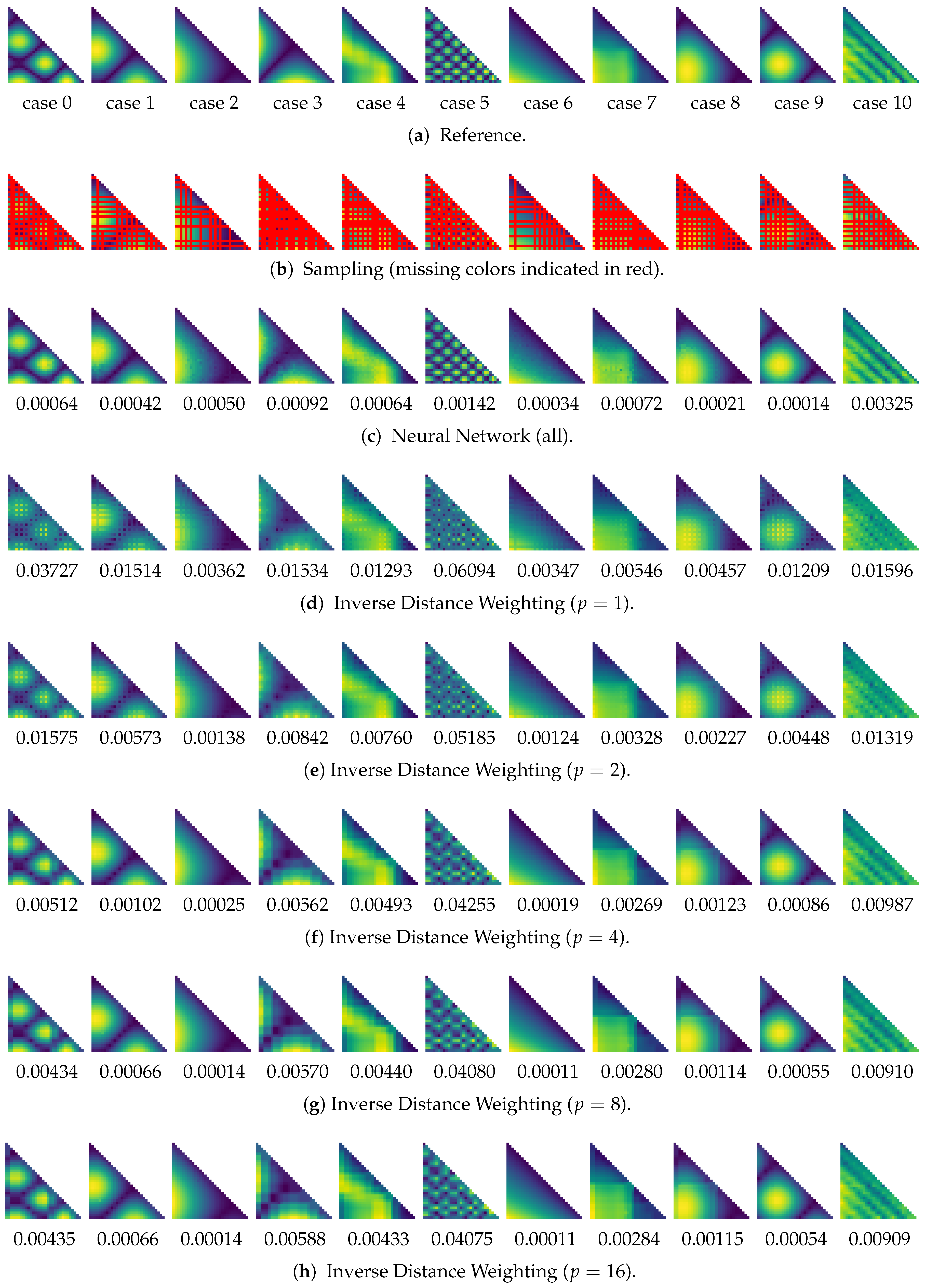
6.3. Similarity Estimation
6.4. Discussion
7. Conclusions
Acknowledgments
Conflicts of Interest
References
- Joshi, A.; Rheingans, P. Illustration-inspired techniques for visualizing time-varying data. In Proceedings of the VIS 05, IEEE Visualization, Minneapolis, MN, USA, 23–28 October 2005; pp. 679–686. [Google Scholar]
- Lee, T.Y.; Shen, H.W. Visualization and Exploration of Temporal Trend Relationships in Multivariate Time-Varying Data. IEEE Vis. Comput. Graph. 2009, 15, 1359–1366. [Google Scholar]
- Joshi, A.; Rheingans, P. Evaluation of illustration-inspired techniques for time-varying data visualization. Comput. Graph. Forum 2008, 27, 999–1006. [Google Scholar] [CrossRef]
- Woodring, J.; Wang, C.; Shen, H.W. High dimensional direct rendering of time-varying volumetric data. In Proceedings of the IEEE Visualization, Seattle, WA, USA, 19–24 October 2003; pp. 417–424. [Google Scholar]
- Balabanian, J.P.; Viola, I.; Möller, T.; Gröller, E. Temporal Styles for Time-Varying Volume Data. In Proceedings of the 3DPVT’08—The Fourth International Symposium on 3D Data Processing, Visualization and Transmission, Atlanta, GA, USA, 18–20 June 2008; Gumhold, S., Kosecka, J., Staadt, O., Eds.; 2008; pp. 81–89. [Google Scholar]
- Bach, B.; Dragicevic, P.; Archambault, D.; Hurter, C.; Carpendale, S. A Descriptive Framework for Temporal Data Visualizations Based on Generalized Space-Time Cubes. Comput. Graph. Forum 2016. [Google Scholar] [CrossRef]
- Fang, Z.; Möller, T.; Hamarneh, G.; Celler, A. Visualization and Exploration of Time-varying Medical Image Data Sets. In Proceedings of the Graphics Interface 2007, Montreal, QC, Canada, 28–30 May 2007; ACM: New York, NY, USA, 2007; pp. 281–288. [Google Scholar]
- Wang, C.; Yu, H.; Ma, K.L. Importance-Driven Time-Varying Data Visualization. IEEE Vis. Comput. Graph. 2008, 14, 1547–1554. [Google Scholar] [CrossRef] [PubMed]
- Widanagamaachchi, W.; Christensen, C.; Bremer, P.T.; Pascucci, V. Interactive exploration of large-scale time-varying data using dynamic tracking graphs. In Proceedings of the IEEE Symposium on Large Data Analysis and Visualization (LDAV), Seattle, WA, USA, 14–15 October 2012; pp. 9–17. [Google Scholar]
- Lee, T.Y.; Shen, H.W. Visualizing time-varying features with TAC-based distance fields. In Proceedings of the 2009 IEEE Pacific Visualization Symposium, Beijing, China, 20–23 April 2009; pp. 1–8. [Google Scholar]
- Silver, D.; Wang, X. Tracking and Visualizing Turbulent 3D Features. IEEE Vis. Comput. Graph. 1997, 3, 129–141. [Google Scholar] [CrossRef]
- Ji, G.; Shen, H.W. Feature Tracking Using Earth Mover’s Distance and Global Optimization. Pac. Graph. 2006. [Google Scholar]
- Weber, G.; Dillard, S.; Carr, H.; Pascucci, V.; Hamann, B. Topology-Controlled Volume Rendering. IEEE Vis. Comput. Graph. 2007, 13, 330–341. [Google Scholar] [CrossRef] [PubMed]
- Narayanan, V.; Thomas, D.M.; Natarajan, V. Distance between extremum graphs. In Proceedings of the IEEE Pacific Visualization Symposium, Hangzhou, China, 14–17 April 2015; pp. 263–270. [Google Scholar]
- Schneider, D.; Wiebel, A.; Carr, H.; Hlawitschka, M.; Scheuermann, G. Interactive Comparison of Scalar Fields Based on Largest Contours with Applications to Flow Visualization. IEEE Vis. Comput. Graph. 2008, 14, 1475–1482. [Google Scholar] [CrossRef] [PubMed]
- Rubner, Y.; Tomasi, C.; Guibas, L. The Earth Mover’s Distance as a Metric for Image Retrieval. Int. J. Comput. Vis. 2000, 40, 99–121. [Google Scholar] [CrossRef]
- Tong, X.; Lee, T.Y.; Shen, H.W. Salient time steps selection from large scale time-varying data sets with dynamic time warping. In Proceedings of the 2012 IEEE Symposium on Large Data Analysis and Visualization (LDAV), Seattle, WA, USA, 14–15 October 2012; pp. 49–56. [Google Scholar]
- Seshadrinathan, K.; Bovik, A.C. Motion Tuned Spatio-temporal Quality Assessment of Natural Videos. IEEE Trans. Image Process. 2010, 19, 335–350. [Google Scholar] [CrossRef] [PubMed]
- Correa, C.D.; Ma, K.L. Dynamic Video Narratives. ACM Trans. Graph. 2010, 29, 88. [Google Scholar] [CrossRef]
- Lu, A.; Shen, H.W. Interactive Storyboard for Overall Time-Varying Data Visualization. In Proceedings of the 2008 IEEE Pacific Visualization Symposium, Kyoto, Japan, 5–7 March 2008; pp. 143–150. [Google Scholar]
- Post, F.H.; Vrolijk, B.; Hauser, H.; Laramee, R.S.; Doleisch, H. The State of the Art in Flow Visualisation: Feature Extraction and Tracking. Comput. Graph. Forum 2003, 22, 775–792. [Google Scholar] [CrossRef]
- McLoughlin, T.; Laramee, R.S.; Peikert, R.; Post, F.H.; Chen, M. Over Two Decades of Integration-Based, Geometric Flow Visualization. Comput. Graph. Forum 2010, 29, 1807–1829. [Google Scholar] [CrossRef]
- Garces, E.; Agarwala, A.; Gutierrez, D.; Hertzmann, A. A Similarity Measure for Illustration Style. ACM Trans. Graph. 2014, 33, 93. [Google Scholar] [CrossRef]
- Frey, S.; Ertl, T. Progressive Direct Volume-to-Volume Transformation. IEEE Trans. Vis. Comput. Graph. 2017, 23, 921–930. [Google Scholar] [CrossRef] [PubMed]
- Frey, S.; Ertl, T. Fast Flow-based Distance Quantification and Interpolation for High-Resolution Density Distributions. In Proceedings of the EG 2017 (Short Papers), Lyon, France, 24–28 April 2017. [Google Scholar]
- Frey, S.; Ertl, T. Flow-Based Temporal Selection for Interactive Volume Visualization. Comput. Graph. Forum 2016. [Google Scholar] [CrossRef]
- Marwan, N.; Carmenromano, M.; Thiel, M.; Kurths, J. Recurrence plots for the analysis of complex systems. Phys. Rep. 2007, 438, 237–329. [Google Scholar] [CrossRef]
- Vasconcelos, D.; Lopes, S.; Viana, R.; Kurths, J. Spatial recurrence plots. Phys. Rev. E 2006, 73. [Google Scholar] [CrossRef] [PubMed]
- Marwan, N.; Kurths, J.; Saparin, P. Generalised recurrence plot analysis for spatial data. Phys. Lett. A 2007, 360, 545–551. [Google Scholar] [CrossRef]
- Bautista-Thompson, E.; Brito-Guevara, R.; Garza-Dominguez, R. RecurrenceVs: A Software Tool for Analysis of Similarity in Recurrence Plots. In Proceedings of the Electronics, Robotics and Automotive Mechanics Conference 2008, Morelos, Mexico, 30 September–3 October 2008; pp. 183–188. [Google Scholar]
- Frey, S.; Sadlo, F.; Ertl, T. Visualization of temporal similarity in field data. IEEE Trans. Vis. Comput. Graph. 2012, 18, 2023–2032. [Google Scholar] [CrossRef] [PubMed]
- Goodfellow, I.; Bengio, Y.; Courville, A. Deep Learning; The MIT Press: Cambridge, MA, USA, 2016. [Google Scholar]
- Hu, H.; Holman, P.M.; de Haan, G. Image interpolation using classification-based neural networks. In Proceedings of the IEEE International Symposium on Consumer Electronics, Reading, UK, 1–3 September 2004; pp. 133–137. [Google Scholar]
- Plaziac, N. Image Interpolation Using Neural Networks. IEEE Trans. Image Proccess. 1999, 8, 1647–1651. [Google Scholar] [CrossRef] [PubMed]
- Chen, C.H.; Kuo, C.M.; Yao, T.K.; Hsieh, S.H. Anisotropic Probabilistic Neural Network for Image Interpolation. J. Math. Imag. Vis. 2014, 48, 488–498. [Google Scholar] [CrossRef]
- Guillaumin, M.; Verbeek, J.J.; Schmid, C. Is that you? Metric learning approaches for face identification. In Proceedings of the 2009 IEEE 12th International Conference on Computer Vision, Kyoto, Japan, 29 September–2 October 2009; pp. 498–505. [Google Scholar]
- Kulis, B. Metric Learning: A Survey. Found. Trends Mach. Learn. 2013, 5, 287–364. [Google Scholar] [CrossRef]
- Davis, J.V.; Kulis, B.; Jain, P.; Sra, S.; Dhillon, I.S. Information-theoretic metric learning. In Proceedings of the 24th International Conference on Machine Learning, Corvalis, OR, USA, 20–24 June 2007; pp. 209–216. [Google Scholar]
- Velten, A.; Wu, D.; Jarabo, A.; Masia, B.; Barsi, C.; Joshi, C.; Lawson, E.; Bawendi, M.; Gutierrez, D.; Raskar, R. Femto-photography: Capturing and Visualizing the Propagation of Light. ACM Trans. Graph. 2013, 32, 44. [Google Scholar] [CrossRef]
- Kingma, D.P.; Ba, J. Adam: A Method for Stochastic Optimization. axiv 2014, arXiv:1412.6980. [Google Scholar]
- Abadi, M.; Agarwal, A.; Barham, P.; Brevdo, E.; Chen, Z.; Citro, C.; Corrado, G.S.; Davis, A.; Dean, J.; Devin, M.; et al. TensorFlow: Large-Scale Machine Learning on Heterogeneous Systems. Available online: tensorflow.org (accessed on 22 August 2017).


© 2017 by the author. Licensee MDPI, Basel, Switzerland. This article is an open access article distributed under the terms and conditions of the Creative Commons Attribution (CC BY) license (http://creativecommons.org/licenses/by/4.0/).
Share and Cite
Frey, S. Sampling and Estimation of Pairwise Similarity in Spatio-Temporal Data Based on Neural Networks. Informatics 2017, 4, 27. https://doi.org/10.3390/informatics4030027
Frey S. Sampling and Estimation of Pairwise Similarity in Spatio-Temporal Data Based on Neural Networks. Informatics. 2017; 4(3):27. https://doi.org/10.3390/informatics4030027
Chicago/Turabian StyleFrey, Steffen. 2017. "Sampling and Estimation of Pairwise Similarity in Spatio-Temporal Data Based on Neural Networks" Informatics 4, no. 3: 27. https://doi.org/10.3390/informatics4030027
APA StyleFrey, S. (2017). Sampling and Estimation of Pairwise Similarity in Spatio-Temporal Data Based on Neural Networks. Informatics, 4(3), 27. https://doi.org/10.3390/informatics4030027