Bus Operations Scheduling Subject to Resource Constraints Using Evolutionary Optimization


NEC Laboratories Europe, 69115 Heidelberg, Germany
*
Author to whom correspondence should be addressed.
†
Current address: Kurfuersten Anlage 36, 69115 Heidelberg, Germany.
‡
These authors contributed equally to this work.
Informatics 2018, 5(1), 9; https://doi.org/10.3390/informatics5010009
Submission received: 19 December 2017
/
Revised: 28 January 2018
/
Accepted: 2 February 2018
/
Published: 6 February 2018
(This article belongs to the Special Issue IoT and Informatics Applications in Logistics and Intelligent Transportation Systems)
Abstract
:In public transport operations, vehicles tend to bunch together due to the instability of passenger demand and traffic conditions. Fluctuation of the expected waiting times of passengers at bus stops due to bus bunching is perceived as service unreliability and degrades the overall quality of service. For assessing the performance of high-frequency bus services, transportation authorities monitor the daily operations via Transit Management Systems (TMS) that collect vehicle positioning information in near real-time. This work explores the potential of using Automated Vehicle Location (AVL) data from the running vehicles for generating bus schedules that improve the service reliability and conform to various regulatory constraints. The computer-aided generation of optimal bus schedules is a tedious task due to the nonlinear and multi-variable nature of the bus scheduling problem. For this reason, this work develops a two-level approach where (i) the regulatory constraints are satisfied and (ii) the waiting times of passengers are optimized with the introduction of an evolutionary algorithm. This work also discusses the experimental results from the implementation of such an approach in a bi-directional bus line operated by a major bus operator in northern Europe.
1. Introduction
During the scheduling phase of bus services, a set of conflicting objectives are optimized such as the operational costs and the waiting times of passengers at stops. However, due to many exogenous factors, such as road traffic and spatio-temporal passenger demand variations, the optimal schedule does not perform as anticipated, resulting in bus bunching phenomena. This unreliability leads to passenger dissatisfaction and to additional operational costs for the service provider. Therefore, several research works related to bus bunching have tried to address the service reliability problem (Gkiotsalitis and Cats [1], Chapman and Michel [2], Pilachowski [3], Gkiotsalitis and Maslekar [4]).
In several cities where the timetables of bus services are not strictly followed, a number of informal methods have been utilized for maintaining the service reliability. In Chile for instance, drivers are assisted by an informal group of independent information intermediaries, known as “Sapos”, who record the arrival time of buses and inform the subsequent drivers in order to help them maintain uniform headways (Johnson et al. [5]). These labor-intensive practices of maintaining reliability in bus operations become inefficient when the frequency of trips is very high. This study focuses specifically on such high frequency services with dispatching headways between consecutive bus trips of less than 15 min since several studies (Randall et al. [6], Welding [7]) have shown that the arrivals of passengers at stops are not random and are tailored to the scheduled arrival times of bus trips in the case of low frequency services.
The advent of new monitoring technologies such as in-vehicle telematics and automated fare collection systems has revolutionized the monitoring capabilities of the transit service operations. Nowadays, the monitoring capabilities of the passenger waiting times at stops have been increased and, given this new information, bus operators strive to improve the reliability of their daily operations.
In past years, several methodologies were developed for enhancing the reliability of transit services. Eberlein [8] explained three ways of controlling the headways: (a) Station-control strategies which consist of (i) holding a bus at a stop and (ii) stop-skipping; (b) Interstation-control strategies consisting of speed control and traffic signal priorities and (c) On-demand vehicle addition strategies that add vehicles at some specific points of the bus routes. From the above-mentioned strategies, the first strategy that includes holding and stop skipping is considered to be the most important methodology.
To further explain the bus holding control strategy, a bus trip can be held at specific critical stops (known as control points or time points) in an effort to maintain even headways. In several works, such as the work of Hickman [9], bus holding is proposed as a real-time strategy to avoid bus bunching. The typical objective of a bus holding strategy is to ensure that the waiting times of passengers at stops do not vary significantly from the planned ones. However, recent works, such as the work of Bartholdi and Eisenstein [10], focused on maintaining even headways between bus trips at the locations of the control point stops without adhering to the planned headway values. Although bus holding can be proved beneficial to bus operations, several works have proposed to introduce limitations on holding strategies because extensive holding of bus trips can cause inconvenience to passengers, overcrowding at stops and “schedule sliding” if the bus trips are postponed due to holding (Delgado et al. [11]).
Public transport authorities use the passenger waiting times at stops to evaluate the performance of the operations in the case of high frequency services. In contrast to the low frequency services where the main objective is the service punctuality because passengers try to synchronize their arrival times at stops with the scheduled arrival times of bus trips, in high frequency services the passenger arrival times at stops are random (Welding [7]) and the waiting times of passengers at stops can be directly linked to the headways between consecutive trips (they are considered equal to half the value of the headways). O’Flaherty and Mancan [12] studied the relationship between bus headways and average passenger waiting times in peak and off-peak traffic conditions. The holding problem has been examined as a multi-objective problem in other works such as Barnett [13], where a holding strategy of individual buses at control stops tries to minimize at the same time the passenger waiting times and the delay of on-board passengers. Turnquist [14] studied in more detail the effects of schedule reliability and bus frequency on the waiting times experienced by the passengers. In addition, the stochastic nature of passenger waiting times was considered in the work of Gkiotsalitis and Maslekar [15], where a stochastic search and branch hopping/merging algorithm was used for reducing the excess waiting times of passengers.
Apart from bus holding, a variety of other solution strategies have been proposed for improving the bus operations. Adherence to the planned timetables was proposed by Bates et al. [16] and Daganzo [17] where the latter worked on an adaptive control scheme that focused on achieving target headways by adjusting the bus cruising speed. In such a scheme, when a bus arrives at a control point its headway is compared to a pre-specified target headway value for performing the appropriate adjustment. Other works, such as Friedman [18], have focused only on the dispatching times of bus trips by developing mathematical models to optimize the departure times of buses.
The above-mentioned works focus on specific problems such as the (i) timetable design and the (ii) real-time control. This paper focuses on the first problem of timetable design for high frequency services with a specific target of reducing the passenger waiting time fluctuations and satisfying the resource limitations in terms of fleet size and regulatory constraints. Regulatory constraints such as bus driver meal breaks, layover times and dispatching headway bounds are interconnected and any change in the bus timetables can lead to violations of different constraints. Satisfying the regulatory constraints and minimizing the Excess Waiting Times (EWT) of passengers at control point stops turns the timetabling problem into a discrete, constrained optimization problem which does not exhibit a polynomial computational complexity. For this reason, this paper presents an evolutionary algorithm for exploring the vast solution space under a set of constraint limitations. The performance of the proposed algorithm, the improvement in the timetable design and the improvement of passengers waiting times at stops in real operations under different assumptions of travel time variations are tested in a bi-directional bus line from a major bus operator in northern Europe.
2. Related Work
Yan and Chen [19] developed a model for timetable design by formulating the movement of bus trips and the passenger flows in order to manage the interrelationship between passenger demand and bus trip supply. They formulated the problem as a mixed integer multiple commodity network flow problem and a Lagrangian heuristic algorithm was developed for solving it.
Niu and Tian [20] developed a methodology to determine the dispatching times of bus trips subject to capacity constraints with the use of heuristic algorithms. This methodology was based on the concept that a constant headway cannot satisfy effectively the time-dependent passenger demand. In contrary, an irregular schedule that allows uneven headways might be able to accommodate the dynamic demand patterns. The operational time was divided into various equal time periods to formulate the transit scheduling problem. Considering the dwell times and the trip travel times, the dispatching time of each bus trip was calculated subject to inequality constraints that belong to the specific operational time period. The objectives were the reduction of passenger waiting times and the reduction of the number of vehicles leading to a bi-objective function which is also adopted by other works such as Gkiotsalitis and Cats [21] and Ceder et al. [22]. In particular, Ceder et al. [22] followed this bi-objective optimization approach for minimizing headway deviations and passenger loads at the same time using a graphical heuristic approach.
Sun et al. [23] explored the idea of using a flexible timetable optimization based on hybrid vehicle sizes in order to address the travel demand fluctuations. This study compared operational strategies like total travel times and total costs of using large size or smaller size buses at different time periods such as peak and off-peak periods. Following this approach, the total in-vehicle time cost and the waiting time cost at stops were considered. In addition, an optimization model considering hybrid, large and smaller-size vehicles was solved with the use of an adaptive heuristic algorithm. From the results, it was observed that a hybrid bus schedule providing the benefits of both large and smaller size vehicles can be implemented for reducing the operational costs and managing the passenger demand more efficiently. Nevertheless, limitations in resources such as the availability of different bus types might restrict the applicability of such a method in practical problems.
Chen [24] defined a timetable setting problem to determine the dispatching time of bus trips based on the flow intensity of passengers. This method minimized the total waiting time of passengers at stops by determining the number of bus trips for each time period and the dispatching times of these trips using dynamic optimization. Using dynamic programming, the arrangements of bus trips were designed as a multi-stage optimization problem which was optimized by finding the global optimal solution. The dispatching times of bus trips were computed by considering the passenger flow intensity, the available resources and the operational costs for each optimization time period.
More recently, Gkiotsalitis and Stathopoulos [25] developed a method for modifying the dispatching times of trips in order to reduce the waiting time deviation of passengers at stops and synchronize the arrival times of buses at specific stops with the starting times of activities (i.e., major events that can be derived from social media data (Gkiotsalitis and Stathopoulos [26])). This multi-objective optimization was treated as a single-objective optimization problem with the use of weight factors for each one of the main objectives.
Other works related to timetable design for railway services, such as Shi et al. [27], utilized also the minimization of passenger waiting times as the main problem objective. The focus of such works was on loop-shaped lines that connect several radial lines together; thereby, enhancing the accessibility of the rail network. For enhancing the accessibility of the rail network, Shi et al. [27] formulated a bi-objective function considering the waiting times at the stops of the line together with the waiting times related to passenger transfers subject to constraints such as total trip times, departure times, headways to be maintained, arrival times and dwell times. This formulation resulted in a nonlinear programming problem which was also non-convex. Hence a genetic algorithm was applied and was effective in reducing the passenger waiting times. However, the optimization during off-peak periods was more effective than the peak periods due to the shorter headways that are exhibited during the peak periods.
It is also worth noting that several other works from the field of logistics (i.e., Cattaruzza et al. [28], Du et al. [29]) focus on developing daily schedules for deliveries with the objective of reducing the operational costs while satisfying all delivery requests. Nevertheless, a distinct difference between the delivery scheduling problems and the transit timetabling problems is the inclusion of multiple vehicle routing sub-problems in the scheduling phase of the former.
The majority of the previous timetable optimization approaches have developed methodologies to optimize passenger waiting times without an in-depth consideration of the resource limitations of the transit service providers. For instance, many times it is impractical to introduce new trips in a route in order to meet the passenger demand fluctuations given the inherent resource limitations. This paper explores this area by including resource constraints such as driver meal and resting times in the problem definition and developing a Genetic Algorithm (GA) to optimize the resulting objective function as it is presented in the next sections.
3. Modelling the Multi-Constrained Scheduling Problem
Buses are assigned to a service route during the frequency setting phase of transit planning. The problem of timetable optimization is formulated by considering the expected trip travel times and the resource limitations of bus lines. A timetable can be represented by a two-dimensional matrix denoted as D. This matrix has dimensions where represents the number of planned trips for the day and denotes the number of stops in the line. Every element in the matrix D represents the scheduled time of arrival of bus trip i at stop j in minutes. In order to simplify the notation, the arrival time and the departure time differ by s following the work of Dueker et al. [30] which observed that a typical dwell time is in the range of s. For improving the efficiency of bus services, the dispatching times of buses are modified to create an optimized schedule. Table 1 presents the common notation used in this work for modelling the multi-constrained bus scheduling problem.
3.1. Passenger Excess Waiting Times
The Excess Waiting Times (EWT) of passengers at control point stops is the key performance index in bus schedule optimization problems of high frequency services. EWT is the time spent waiting for the bus due to the bus headway deviations from their target values. The EWT of the entire service is a linear weighted function of the EWTs of passengers at different stops during different periods of day.
The bus service performance is measured in terms of daily EWT values in several cities with high frequency services such as London (TfL [31]) and Singapore (LTA [32]). The EWT targets the improvement of the service reliability from the passengers side, rather than the service provider’s side as explained in van Oort [33]. For calculating the waiting time variance of passengers over the entire day, transport authorities in metropolises such as London and Singapore use the following formula:
where is time of arrival of the ith trip at jth stop in minutes. The EWT depends on the scheduled arrival time of buses at each stop. The EWT function of Equation (1) is nonlinear and this increases the complexity of the optimization problem. In order to improve the reliability of the service without introducing new trips, the only available control measure at the timetable design phase is the modification of the dispatching times of bus trips.
Apart from the EWTs of passengers, transportation authorities impose regulatory constraints for the bus services. These constraints should be satisfied during the timetable design phase and a set of such regulatory constraints is described in the remainder of this section.
3.2. Dispatching Headway Range Constraint
A first requirement from transport authorities is that buses from the same line should not be dispatched simultaneously. In addition, the dispatching times of consecutive bus trips should not exceed the predefined target of bus dispatching time intervals. These two requirements establish a lower and upper limit for the dispatching times of consecutive bus trips. These lower and upper limits for the dispatching headways of successive trips can vary during different time periods of the day since the service frequency is typically higher during peak times and lower during off-peak periods. The upper limit of dispatching headways is denoted as and the lower limit as . Therefore, the dispatching times of two consecutive bus trips i, should satisfy the following inequality:
where and are the dispatching times of trips i and . It is worth mentioning that Equation (2) assumes that the lower and upper dispatching limits are stable throughout the day; however, their values can vary for different time periods of the day based on the frequency setting requirements without loss of generality.
3.3. Layover Time Constraint
Every daily trip operated by a bus driver should enjoy a specific time period of recovery before the next trip operated by the same driver starts. This resting time requirement for the driver is a layover time which can vary from zero to several minutes. A layover time l can be integrated into the mathematical model in the form of an inequality constraint:
where denotes the scheduled departure time of the ith trip and denotes the scheduled arrival time of the previous trip operated by the same bus driver at the last stop. This inequality constraint ensures that the bus driver will rest for a time period which is at least equal to the layover time l before starting his/her next trip.
3.4. Mealtime Constraint
Another typical regulatory constraint is the meal time constraint which ensures that a bus driver has an adequate break during a specific time of the day. The meal time duration, M, is fixed by the transport authorities and can form the following set of inequality constraints:
where denotes the scheduled departure time of the trip and denotes the scheduled arrival time of the previous trip operated by the same bus driver who had to take a meal time break at the last stop.
3.5. Departure Time Constraint
This constraint ensures that the dispatching times of the first and the final trip of the day cannot be modified for avoiding “schedule sliding”. Following this approach, the total duration of the daily trips is strictly regulated and the daily operations are not prolonged; this is something that could have implicated the rostering of bus drivers. The constraints have the following form:
where is the dispatching time of the first trip of the day and the dispatching time of the last trip of the day.
3.6. Mathematical Program of the Timetabling Problem
The service-wide excess waiting times of passengers presented in Equation (1) is the objective function of our problem which can be written in the standard form by introducing the full set of regulatory constraints as:
As it is evident from the problem definition of Equation (6), the decision variables of the problem are the arrival times of bus trips at stops, D. However, the arrival time of a trip at one stop is defined based on the travel times between bus stops that can be derived from the analysis of historical Automated Vehicle Location (AVL) data. Therefore, the arrival time of a trip at a stop cannot be decided directly from the bus operator. To the contrary, the bus operator can define the dispatching times of trips during the timetabling phase and these dispatching times can modify the respective arrival times at stops. As a result, the following equality constraint is added to the problem of Equation (6):
where Equation (7) denotes that the arrival time of a bus trip i at stop is equal to the dispatching time of that trip, , plus the estimated link travel times and dwell times from the departure stop until stop s.
The objective function of Equation (6) is a non-convex function and computing the global optimum of such a function is a computational intractable problem. The decision variables of the timetabling problem, which are the dispatching times of trips, can take discrete values because a timetable is expressed in minutes and applying exhaustive enumeration for finding the optimal dispatching times can be practical only for small-scale problems due to the exponential computational cost of simple enumeration.
3.7. Exterior Point Penalties for Multi-Constrained Scheduling
The computed timetable that minimizes the EWTs of passengers should satisfy all regulatory constraints. Due to the presence of numerous equality and inequality constraints, an exterior point penalty method is adopted. Penalty methods (known also as barrier methods) use penalties and weights for transforming constrained optimization problems to unconstrained ones by adding the constraints to the objective function which ideally converges to the solution of the original constrained problem. The new objective function that uses exterior point penalties is called penalty function and such penalty functions are widely used in software packages for constrained optimization problems. In our problem, the objective function of Equation (6) together with the associated constraints can be reformulated as:
where is the total number of inequality constraints and the total number of equality constraints presented in Equations (6) and (7). In addition represents the value of the constraint for a specific set of arrival times at stops, D. For instance, if the constraint refers to the equality constraint , then . If then this constraint is violated and penalizes the penalty function by a value of where is a weight factor for ensuring that the constraints have more impact to the penalty function than the objective function score and are prioritized during the optimization process.
Similarly, represents the value of the inequality constraint for a specific set of arrival times at stops, D. To provide a tangible example, if the inequality constraint is , then . If , then this inequality constraint is violated. At the same time, and the penalty function value increases by . In contrary, if , then the inequality constraint is satisfied and the penalty function remains unaffected since .
As it is evident from the analysis, the penalty function is formed in such a way that its score is increased progressively when a constraint is violated and remains unaffected when a constraint is satisfied. The constraints of Equation (8) are also interrelated and satisfying one constraint might lead to the violation of another or to the increase of passengers’ EWTs.
4. Solution Method-Evolutionary Optimization
The timetabling problem is formulated as a discrete unconstrained optimization problem with a non-convex penalty function that needs to be minimized. The non-convexity of the penalty function reduces the probability of finding the global optimum solution with exact optimization methods; whereas, its discrete nature makes the optimization process very slow and prohibits its solution in polynomial time. Therefore, this section proposes a Genetic Algorithm (GA) tailored to the specific needs of the timetabling problem for finding an approximation to the global optimum solution.
GAs explore the solution space by focusing on the structure of the problem instead of the form of the function that needs to be minimized. Therefore, they have better performance for problems where the minimized function is non-convex and the problem at hand is a complex, multi-variate one (De-rong et al. [34]).
The proposed GA algorithm utilizes problem-specific mutations that help to reduce the computational cost. The GA starts the optimization from an initial random guess. The initial random guess is a solution to the problem which is not optimal and is selected randomly. For instance, a random guess can be a set of randomly selected dispatching times for all trips .
Starting from an initial random guess, the GA evaluates the value of the penalty function for such a solution and tries to reduce this value by modifying the dispatching times of the initial random guess. The dispatching times can be modified by introducing small changes to the dispatching times of the random guess solution and the GA optimizes the multi-constrained timetabling problem by selecting the elite offspring of each generation. The evolution to new generations follows a greedy rule that does not permit the generation of inferior offsprings; thus, ensuring that the penalty function score cannot increase from generation to generation.
In order to reduce the penalty function value, the dispatching times of the random guess can be modified by a value of up to minutes. Given also the requirement of discrete dispatching times that should be expressed in minutes, each dispatching time modification can receive values from the set where is expressed in minutes.
The dispatching time modifications affect the arrival times of the bus trips at the following stops as expressed in Equation (7). This results in a new timetable, D, and the penalty function value for such timetable, , can be computed for understanding if such change is in the right direction.
The developed GA is specific to the timetabling problem. The GA starts by evaluating the penalty function value for the initial random guess. The initial random guess is considered as the first parent of the GA and can be denoted as A. Its penalty function score then is where is the matrix of bus arrival times at stops when using the dispatching times of the initial random guess. Then, another random solution can be generated forming the second parent of the GA which can be denoted as B and its penalty function value is .
The GA then starts a crossover in which small subsets of trips (“genes”) from parents A and B are exchanged between them in a random manner. The number of exchanged trips is dynamically updated based on the influence of the exchange to the minimization of the penalty function score. The fitness value of the generated offspring is evaluated after the exchange and if there is no improvement, the recombination of the parents continuous with a different number of exchanged genes until an improvement is observed. This approach differs from the typical crossover phase of a GA where the genes of the two parents are exchanged at a random crossover point as it is presented in Figure 1 (Shrestha and Mahmood [35]).
After the crossover phase which results in an offspring that has a better fitness than its parents, a mutation is performed on the dataset. Two types of mutation are developed for the optimization problem. The first type is an educated mutation which tries to satisfy the entirety of layover constraints by modifying the dispatching times of trips that violate the layover constraints. The second mutation type focuses on changing the dispatching times of a set of trips which is selected based on the common genes detection method proposed by Tsai et al. [36]. This method helps to reduce the search space of the algorithm and speed up the optimization process.
With each new generation, the penalty function score is either reduced or is equal to its previous levels. This process continues by updating the parents and the evolution terminates when the penalty function cannot be reduced further. It should be noted here that the reduction of the penalty function score from generation to generation does not guarantee that the EWT of passengers is also reduced. For instance, modifying the dispatching times of trips can reduce the value of the penalty function if several constraints are satisfied even if the EWTs of passengers are increased for such modifications. Nevertheless, when all constraints are satisfied, the penalty function value and the value of the EWTs of passengers are equal because the penalties of the constraints are equal to zero. Therefore, after finding a solution which satisfies all constraints, it is guaranteed that every reduction to the penalty function results in an equivalent reduction to the EWT of passengers.
5. Case Study
Schedule Optimization of a Bi-Directional Bus Service
In this case study, the timetable of a bi-directional bus line from a major bus operator in northern Europe is optimized. This bi-directional service has nine (9) control point stops where the EWT of passengers is monitored. In addition, a total number of 224 trips are allocated to this service and the objective is to define their optimal dispatching times for minimizing the EWTs of passengers at the 9 control point stops while satisfying the full set of regulatory constraints. From the 224 trips, 112 trips are allocated to direction 1 and 112 trips to direction 2.
For computing the optimal dispatching times, the travel times of bus trips between the control points are estimated with the use of Automated Vehicle Location (AVL) data gathered over a 4-month period. Travel times in transport networks can vary significantly over different time periods of the day due to road traffic and passenger demand fluctuations (Dorbritz et al. [37]). This is evident in our analysis of historical AVL data, the results of which are presented in Figure 2. Figure 2 presents the estimated travel times between control stops for all daily trips. In direction 1, the travel times between control point stops 6 and 7 have the highest values of 19–22 min which peak between trips 3 to 25 and trips 76 to 85. A similar pattern can be observed between control point stops 3 and 4 from the 118th trip to the 126th and from the 180th to the 200th. The lowest travel time is observed between control point stops 1 and 2 and control point stops 5 and 6 as well as control point stops 8 and 9 on both directions.
Given the limitations of the available 4-month AVL data, this study used the average values of the observed travel times between control point stops for each bus trip in order to produce timetables in a deterministic manner. At this point, it should be noted that the resulting timetable from this deterministic optimization approach will perform best if the actual travel times of the daily trips are close to their mean values. Nevertheless, this is not always the case and incorporating the stochasticity of travel times to the optimization process might improve the reliability of the resulting timetable. For performing such stochastic optimization, one should analyze historical AVL data from an extensive time period in order to unveil the characteristics of the stochastic nature of travel times for different trip dispatching times (something that can be the scope of a future research work with a specific focus on this aspect).
The resulting timetable of the deterministic optimization process that considers the average travel time values of bus trips between control point stops includes information regarding the arrival times of bus trips at the nine different control point stops of both directions along with details of the trip and bus IDs. The first trip of the day is instructed to start at 5:25 a.m. and the last trip of the day 42 min after midnight (00:42 a.m.). For ease of computation, all day times are converted into minutes. Hence 5:25 a.m. is the 325th min of the day and 00:42 a.m. the 1482th min.
Analyzing the regulatory constraints, the timetable should satisfy the layover constraints which dictate a minimum 9-min break between successive trips operated by the same driver. In addition, at specific times of the day, the bus drivers should have a mandatory mealtime break of at least 23 min. Finally, the ranges of the dispatching headways are divided into four time periods. During each time period the dispatching headways of successive bus trips which are reported at the timetable should be within the range of the lower and upper dispatching headway limits as they are presented in Table 2. From Table 2 it is evident that the examined bus service is a high frequency service and the passengers cannot coordinate their arrivals at stops with the scheduled bus arrivals since the maximum allowed value of dispatching headways is always lower than 16 min; thus, it is reasonable to consider random passenger arrivals.
Although the daily trips start from the 325th min of the day, the mandatory dispatching headway ranges are applied from the 390th min of the day (or from 06:30 a.m.) until the 1380th min of the day (or 11:00 p.m.). The reason behind this is that during the four time periods of the day presented in Table 2, the consecutive dispatching headways should be such that the frequency of the service is in accordance with the peak and off-peak passenger demand patterns for avoiding the under-utilization of buses.
The above-mentioned regulatory constraints introduce a series of equality and inequality constraints into the problem. In an effort to compute an optimal timetable, these constraints are introduced to a penalty function which considers the excess waiting times of passengers at the control point stops according to Equation (8).
The GA described in the previous section is then utilized for optimizing the penalty function. Due to the heuristic nature of the GA, the optimization results can fluctuate significantly throughout the optimization process as it is presented in Figure 3. Figure 3 presents the fluctuation of the penalty function score and the EWT value at each new generation of the GA. Before starting the evolution to new generations, an initial solution guess is randomly selected with an EWT value of 0.297 min. This initial solution guess violates a number of regulatory constraints and exhibits a high penalty function score. Therefore, the GA tries find new offsprings at each generation that have an improved fitness value and reduce the penalty function score.
From Figure 3, it is evident that all constraints are satisfied after 14 generations and at that point the penalty function value is equal to the EWT of passengers at the control point stops (as it is noted by the point P that has a value of 0.44 min). From the beginning of the optimization process until the 14th generation, the EWT of passengers was increased because the GA prioritized the satisfaction of regulatory constraints. After the 14th generation, all regulatory constraints are satisfied and every new generation improves the penalty function score and the EWT of passengers simultaneously because the two functions have become identical. The evolution continuous until the 113th generation because after that generation there are no further improvements at the penalty function score. At that generation, the service-wide excess waiting time of passengers is 0.298 min and the computed timetable satisfies all regulatory constraints. It should be noted here that if the travel times between control point stops were stable throughout the day, the EWT of passengers could have been even closer to zero.
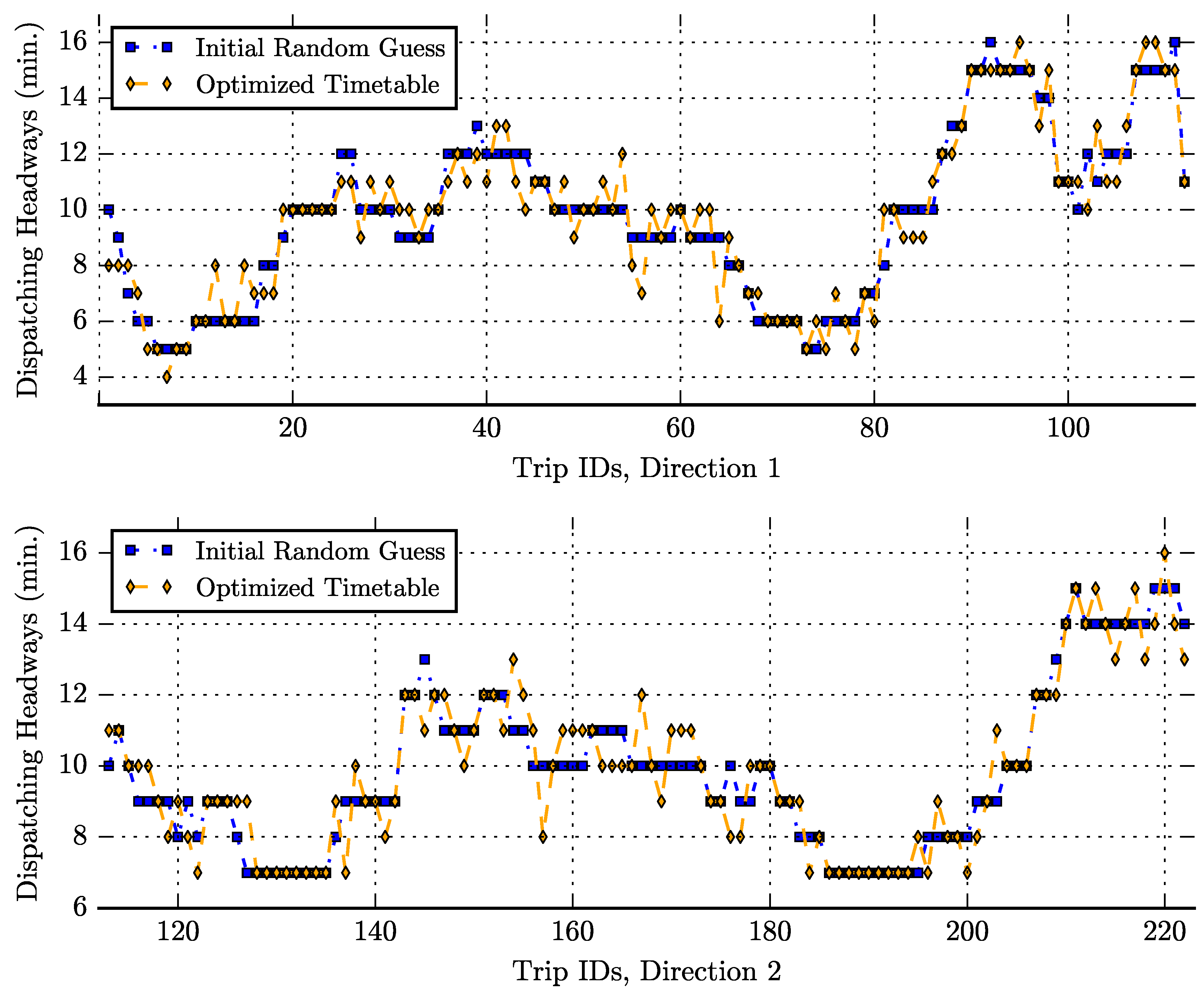
The GA optimization has been programmed in Python 2.7 and has been implemented in a computing machine with a 2.40 GHz processor and 16 GB RAM. After the implementation of the GA, the dispatching headways of consecutive bus trips of the initial random guess solution and the optimized timetable are summarized in Figure 4.
In the initial process of satisfying all the constraints that lasted up to the 14th generation, the interrelation of the regulatory constraints led to constraint asatisfaction trade-offs at each evolution step. Figure 5 presents these constraint satisfaction trade-offs at each generation of the GA. Initially, the vast majority of violated regulatory constraints was related to layover times (31 violations). At the 2nd generation, the dispatching time modifications of the daily trips reduced significantly the layover constraint violations from 31 to 6 but increased slightly the mealtime and dispatching headway range constraints. This trade-off among violated constraints continuous from generation to generation until all constraints are satisfied.
6. Studying the Travel Time Variation Effect in Real Operations Using Simulations
In the previous subsection, the historical AVL data from the bi-directional bus line was used for estimating the travel times between control point stops when computing the optimal timetable. However, the estimated travel times that are used for transport planning purposes can vary significantly from the actual travel times during the daily operations because randomness and heterogeneity are in the nature of traffic phenomena (Hollander and Liu [38]).
The fluctuation of travel times is an important part of transit operations and can impact the reliability of the service. In addition, if travel times vary significantly from their expected values, the scheduled plans might be modified and several regulatory constraints might be violated.
For this reason, the influence of travel time variations during the daily operations to the EWTs of passengers and the regulatory constraints is investigated. During the timetabling phase, the optimal timetable satisfies all regulatory constraints and keeps the EWTs of passengers to a minimum ensuring the service reliability. Nevertheless, during the daily operations the actual travel times can vary significantly from the expected ones and the performance of the service might be compromised.
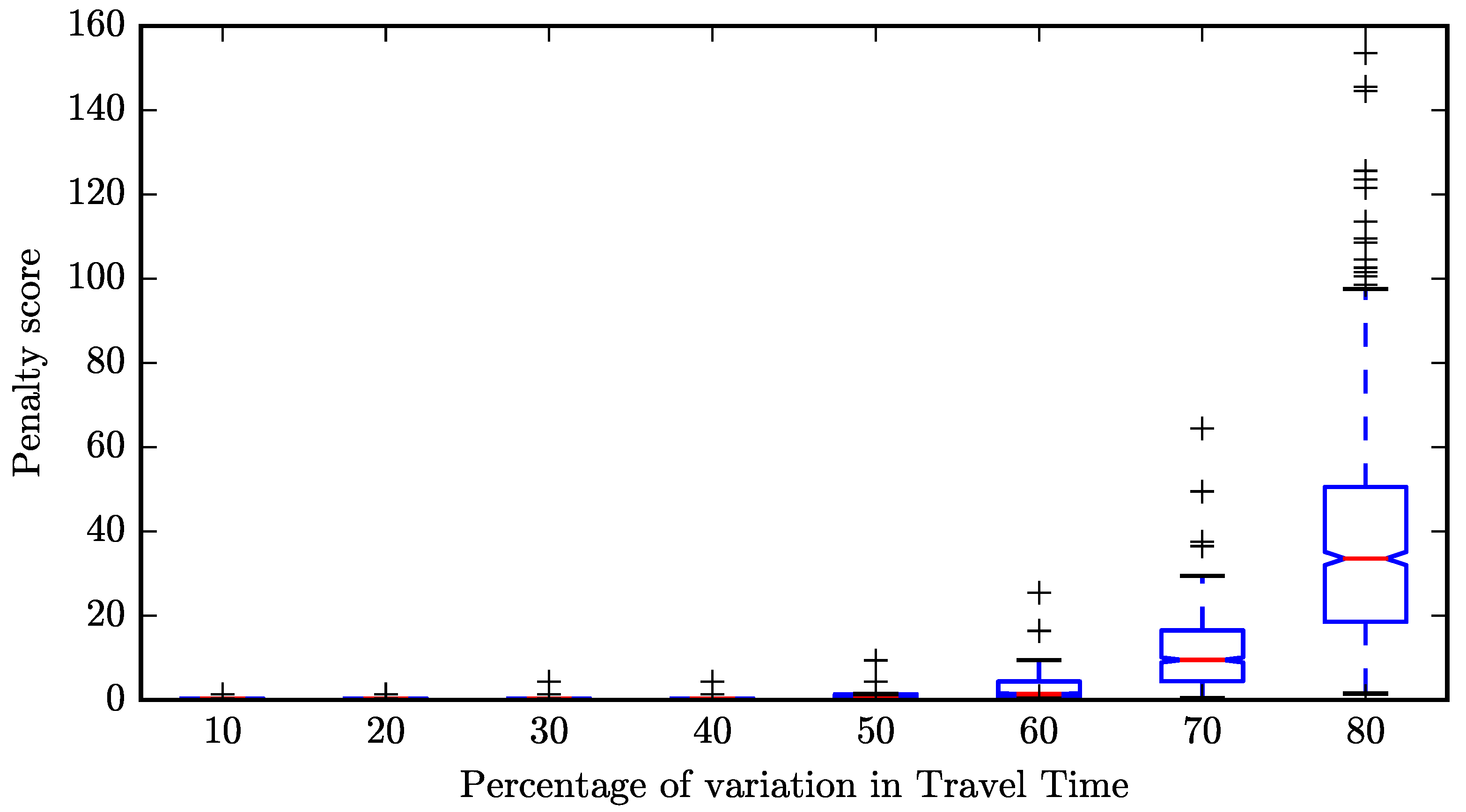
As a realistic service is prone to variation in travel times, it is necessary to study and observe the efficiency of the optimized timetable for different travel time variation scenarios. In order to study this effect, a set of simulation experiments are implemented. In each simulation, the travel times between control point stops are allowed to vary from their expected values by 10%, 20%, 30%, …, 80% and their values are sampled from a normal distribution with mean value equal to the expected travel time value and standard deviation equal to the variation percentage multiplied by the value of the expected travel time. For each one of the scenarios, 1000 simulations are implemented where the link travel times are sampled from the normal distribution and the results are presented in Figure 6 using the Tukey boxplot.
One can observe from Figure 6 that as the percentage of variation in control point travel times increases, the violation of regulatory constraints remains stable up to a point and then increases in a disproportionate fashion. For up to a 50% variation from the expected travel times, the optimal timetable performs well and the regulatory constraints are satisfied during the daily operations. This is an important finding that demonstrates the resilience of the optimal timetable to travel time fluctuations due to exogenous factors. However, if the variance reaches the critical level of 70%, suddenly many regulatory constraints are violated and the optimized timetable does not improve the service at the extent that it should. The same applies also for the case of 80% variation from the expected travel times where the regulatory constraint violations increase disproportionally demonstrating that the optimal timetable cannot keep up with the significant spatio-temporal variations during the actual operations.
7. Results and Concluding Remarks
This study focused on the timetabling problem with the objective of reducing the excess waiting times of passengers at control point stops while satisfying the regulatory constraints. This study utilized information from telematic systems that monitor the daily operations for estimating the travel times between control point stops at different times of the day and computing timetables that can improve the service reliability.
In order to compute the timetables with the use of historical AVL data, the timetabling problem was formulated as a discrete, non-convex and multi-constrained optimization problem. For this reason, a problem-specific GA was developed that updated dynamically the exchange of genes between population members during the crossover phase in order to generate more fit offsprings. This solution method was applied in a bi-directional bus line in north Europe producing a timetable that satisfied all regulatory constraints for an excess waiting time of passengers at the level of 0.298 min as it was presented in Figure 3 and Figure 5. From the analysis, it was observed that:
- All violated constraints were satisfied after a number of population evolutions;
- During the satisfaction of violated constraints, the EWTs of passengers were negatively impacted and were increased by 30%;
- After the satisfaction of constraints, the EWTs of passengers were improved leading to a 0.298-min service-wide EWT.
The EWT value of the optimized timetable will occur in practice if the actual travel times of buses are equal to the estimated ones. However, this is not the case in real-world operations. For instance, well-controlled services with planned timetables that have EWT values close to zero exhibit daily EWTs of 0.8 to 2 min (TfL [39]) in real-world operations. Due to that, this work investigated the impact of the fluctuations of the actual travel times to the EWTs of passengers. In principal, even the smallest travel time fluctuation has the ability to increase the ideal service-wide EWT of 0.298 min of our optimal timetable. For this reason, a simulation-based validation was performed where travel times were allowed to vary from their expected values for 10%, 20%, …, 80%. In this analysis, the service-wide EWT showed resilience for travel time variations of up to 50% but after that point the EWTs and constraint violations were increased in a disproportionate manner. This is a key finding that underlines the importance of addressing exogenous factors such as road traffic and/or road works for maintaining the reliability of the running services.
In future work, the timetabling optimization, which focused on satisfying the regulatory constraints, using AVL-data insights for estimating the travel times, can be expanded even further for improving the excess waiting times of passengers at transfer stops in order to increase the reliability of multi-modal trips. In addition, the stochastic nature of the travel times can be incorporated in the objective function of the timetabling optimization resulting in a stochastic optimization problem with the use of supervised learning methods or by fitting the observed travel times from the archived AVL data to probability distributions. In this way, the reliability improvement potential of stochastically optimized timetables can be further examined. Finally, it is worth examining the potential improvement of the proposed GA convergence rate during the timetabling optimization after incorporating in it advanced hybridization techniques that are described in recent works related to forecasting problems (such as the work of Lopez-Garcia et al. [40] on predicting the short-term travel times in highways).
Author Contributions
K. Gkiotsalitis conceived and designed the experiments; R. Kumar developed analysis tools; R. Kumar performed the experiments and tested the performance of solution methods; K. Gkiotsalitis analyzed the data and the experimental results; K. Gkiotsalitis and R. Kumar wrote the paper.
Conflicts of Interest
The authors declare no conflicts of interest. The founding sponsors had no role in the design of the study; in the collection, analyses, or interpretation of data; in the writing of the manuscript, and in the decision to publish the results.
Abbreviations
The following abbreviations are used in this manuscript:
| AVL | Automated Vehicle Location |
| EA | Evolutionary Algorithm |
| EWT | Excess Waiting Time |
| GA | Genetic Algorithm |
| TMS | Transit Management Systems |
| TT | Travel Time |
References
- Gkiotsalitis, K.; Cats, O. Reliable frequency determination: Incorporating information on service uncertainty when setting dispatching headways. Transp. Res. Part C Emerg. Technol. 2018, 88, 187–207. [Google Scholar] [CrossRef]
- Chapman, R.; Michel, J. Modelling the tendency of buses to form pairs. Transp. Sci. 1978, 12, 165–175. [Google Scholar] [CrossRef]
- Pilachowski, J.M. An Approach to Reducing Bus Bunching; University of California: Berkeley, CA, USA, 2009. [Google Scholar]
- Gkiotsalitis, K.; Maslekar, N. Dynamic Bus Operations Optimization with REFLEX. NEC Tech. J. 2016, 11, 1. [Google Scholar]
- Johnson, R.M.; Reiley, D.H.; Muñoz, J.C. “The War for the Fare”: How Driver Compensation Affects Bus System Performance; Technical Report; National Bureau of Economic Research: Cambridge, MA, USA, 2005. [Google Scholar]
- Randall, E.R.; Condry, B.J.; Trompet, M.; Campus, S.K. International bus system benchmarking: Performance measurement development, challenges, and lessons learned. In Proceedings of the Transportation Research Board 86th Annual Meeting, Washington, DC, USA, 21–25 January 2007. [Google Scholar]
- Welding, P. The instability of a close-interval service. Oper. Res. Soc. 1957, 8, 133–142. [Google Scholar] [CrossRef]
- Eberlein, X.J. Real-time control strategies in transit operations: Models and analysis. Transp. Res. Part A 1997, 1, 69–70. [Google Scholar]
- Hickman, M.D. An analytic stochastic model for the transit vehicle holding problem. Transp. Sci. 2001, 35, 215–237. [Google Scholar] [CrossRef]
- Bartholdi, J.J.; Eisenstein, D.D. A self-coördinating bus route to resist bus bunching. Transp. Res. Part B Methodol. 2012, 46, 481–491. [Google Scholar] [CrossRef]
- Delgado, F.; Munoz, J.C.; Giesen, R. How much can holding and/or limiting boarding improve transit performance? Transp. Res. Part B Methodol. 2012, 46, 1202–1217. [Google Scholar] [CrossRef]
- O’Flaherty, C.; Mancan, D. Bus passenger waiting times in central areas. Traffic Eng. Control 1900, 11, 419–421. [Google Scholar]
- Barnett, A. On controlling randomness in transit operations. Transp. Sci. 1974, 8, 102–116. [Google Scholar] [CrossRef]
- Turnquist, M.A. A model for investigating the effects of service frequency and reliability on bus passenger waiting times. Transp. Res. Rec. 1978, 663, 70–73. [Google Scholar]
- Gkiotsalitis, K.; Maslekar, N. Improving Bus Service Reliability with Stochastic Optimization. In Proceedings of the 2015 IEEE 18th International Conference on Intelligent Transportation Systems (ITSC), Las Palmas, Spain, 15–18 September 2015; pp. 2794–2799. [Google Scholar]
- Bates, J.; Polak, J.; Jones, P.; Cook, A. The valuation of reliability for personal travel. Transp. Res. Part E Logist. Transp. Rev. 2001, 37, 191–229. [Google Scholar] [CrossRef]
- Daganzo, C.F. A headway-based approach to eliminate bus bunching: Systematic analysis and comparisons. Transp. Res. Part B Methodol. 2009, 43, 913–921. [Google Scholar] [CrossRef]
- Friedman, M. A mathematical programming model for optimal scheduling of buses’ departures under deterministic conditions. Transp. Res. 1976, 10, 83–90. [Google Scholar] [CrossRef]
- Yan, S.; Chen, H.L. A scheduling model and a solution algorithm for inter-city bus carriers. Transp. Res. Part A Policy Pract. 2002, 36, 805–825. [Google Scholar] [CrossRef]
- Niu, H.; Tian, X. An approach to optimize the departure times of transit vehicles with strict capacity constraints. Math. Probl. Eng. 2013, 2013. [Google Scholar] [CrossRef]
- Gkiotsalitis, K.; Cats, O. Exact Optimization of Bus Frequency Settings Considering Demand and Trip Time Variations. In Proceedings of the Transportation Research Board 96th Annual Meetings, No: 17-01871, Washington, DC, USA, 8–12 January 2017. [Google Scholar]
- Ceder, A.A.; Hassold, S.; Dano, B. Approaching even-load and even-headway transit timetables using different bus sizes. Public Transp. 2013, 5, 193–217. [Google Scholar] [CrossRef]
- Sun, D.J.; Xu, Y.; Peng, Z.R. Timetable optimization for single bus line based on hybrid vehicle size model. J. Traffic Transp. Eng. 2015, 2, 179–186. [Google Scholar] [CrossRef]
- Chen, Q. Global optimization for bus line timetable setting problem. Discret. Dyn. Nat. Soc. 2014, 2014. [Google Scholar] [CrossRef]
- Gkiotsalitis, K.; Stathopoulos, A. Demand-responsive public transportation re-scheduling for adjusting to the joint leisure activity demand. Int. J. Transp. Sci. Technol. 2016, 5, 68–82. [Google Scholar] [CrossRef]
- Gkiotsalitis, K.; Stathopoulos, A. Joint leisure travel optimization with user-generated data via perceived utility maximization. Transp. Res. Part C Emerg. Technol. 2016, 68, 532–548. [Google Scholar] [CrossRef]
- Shi, R.J.; Mao, B.H.; Ding, Y.; Bai, Y.; Chen, Y. Timetable optimization of rail transit loop line with transfer coordination. Discret. Dyn. Nat. Soc. 2016, 2016. [Google Scholar] [CrossRef]
- Cattaruzza, D.; Absi, N.; Feillet, D.; González-Feliu, J. Vehicle routing problems for city logistics. EURO J. Transp. Logist. 2017, 6, 51–79. [Google Scholar] [CrossRef]
- Du, T.C.; Li, E.Y.; Chou, D. Dynamic vehicle routing for online B2C delivery. Omega 2005, 33, 33–45. [Google Scholar] [CrossRef]
- Dueker, K.J.; Kimpel, T.J.; Strathman, J.G.; Callas, S. Determinants of bus dwell time. J. Public Transp. 2004, 7, 2. [Google Scholar]
- TfL Transport for London: Bus Routes and Borough Reports. Available online: https://www.tfl.gov.uk/forms/14144.aspx (accessed on 1 December 2017).
- LTA Land Transport Authority: Bus Service Reliability Framework. Available online: http://www.lta.gov.sg/data/apps/news/press/2014/20140124BSRF(final2)-Annex.pdf (accessed on 1 December 2017).
- Van Oort, N. Incorporating service reliability in public transport design and performance requirements: International survey results and recommendations. Res. Transp. Econ. 2014, 48, 92–100. [Google Scholar] [CrossRef]
- De-rong, T.; Jing, W.; Han-bo, L.; Xing-wei, W. The optimization of bus scheduling based on genetic algorithm. In Proceedings of the 2011 International Conference on Transportation, Mechanical, and Electrical Engineering (TMEE), Changchun, China, 16–18 December 2011; pp. 1530–1533. [Google Scholar]
- Shrestha, A.; Mahmood, A. Improving Genetic Algorithm with Fine-Tuned Crossover and Scaled Architecture. J. Math. 2016, 2016. [Google Scholar] [CrossRef]
- Tsai, C.W.; Tseng, S.P.; Chiang, M.C.; Yang, C.S.; Hong, T.P. A high-performance genetic algorithm: Using traveling salesman problem as a case. Sci. World J. 2014, 2014. [Google Scholar] [CrossRef] [PubMed]
- Dorbritz, R.; Lüthi, M.; Weidmann, U.; Nash, A. Effects of onboard ticket sales on public transport reliability. In Transportation Research Record: Journal of the Transportation Research Board; The National Academies of Sciences, Engineering, and Medicine: Washington, DC, USA, 2009; pp. 112–119. [Google Scholar]
- Hollander, Y.; Liu, R. Estimation of the distribution of travel times by repeated simulation. Transp. Res. Part C Emerg. Technol. 2008, 16, 212–231. [Google Scholar] [CrossRef]
- TfL Bus Routes & Borough Reports. Available online: https://tfl.gov.uk/forms/14144.aspx?borough=Barking+ (accessed on 1 December 2017).
- Lopez-Garcia, P.; Onieva, E.; Osaba, E.; Masegosa, A.D.; Perallos, A. A hybrid method for short-term traffic congestion forecasting using genetic algorithms and cross entropy. IEEE Trans. Intell. Transp. Syst. 2016, 17, 557–569. [Google Scholar] [CrossRef]
Figure 1.
Dynamically updated exchange of genes between population members.
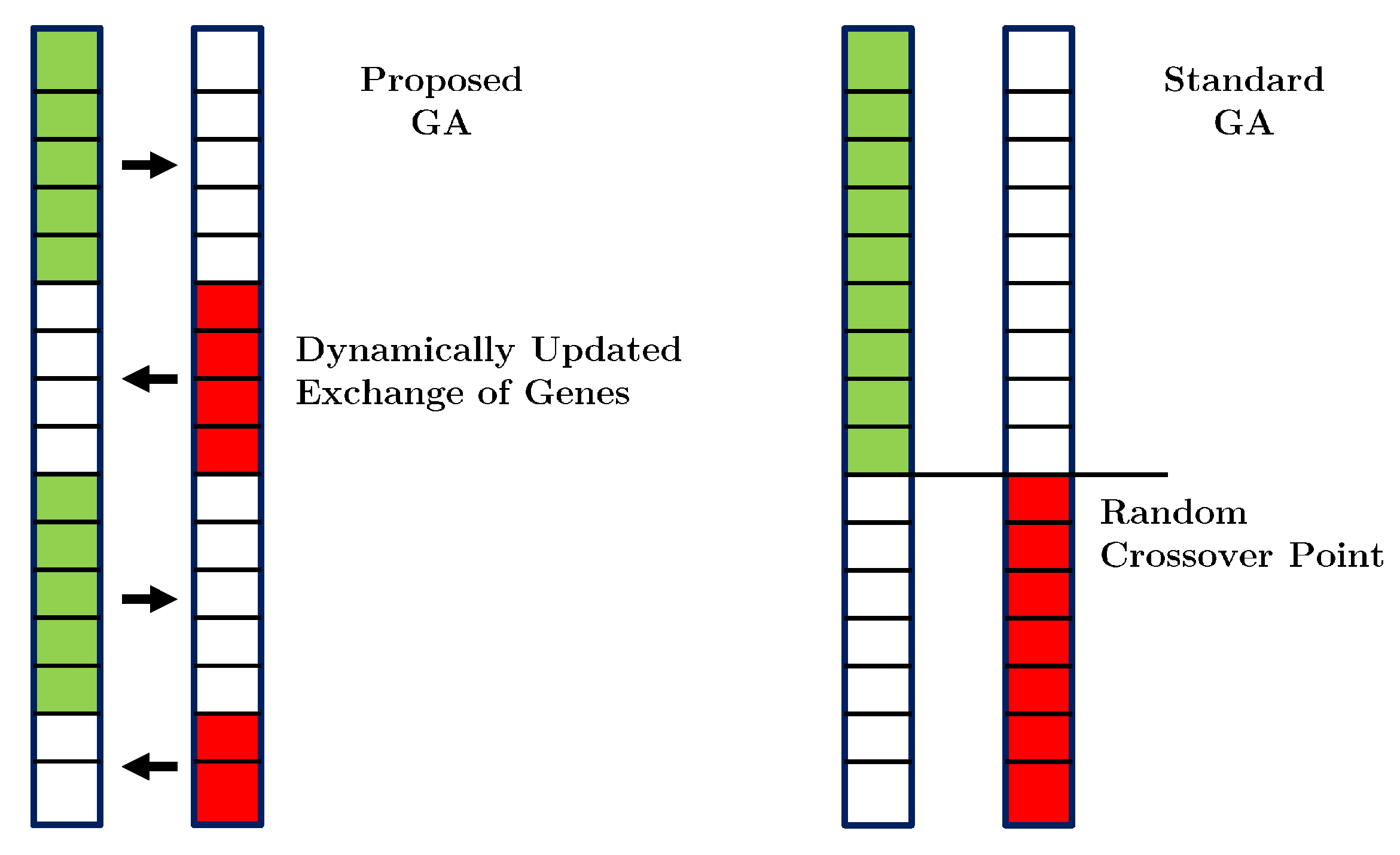
Figure 2.
Estimation of Travel Times between control point stops in minutes for all daily trips.
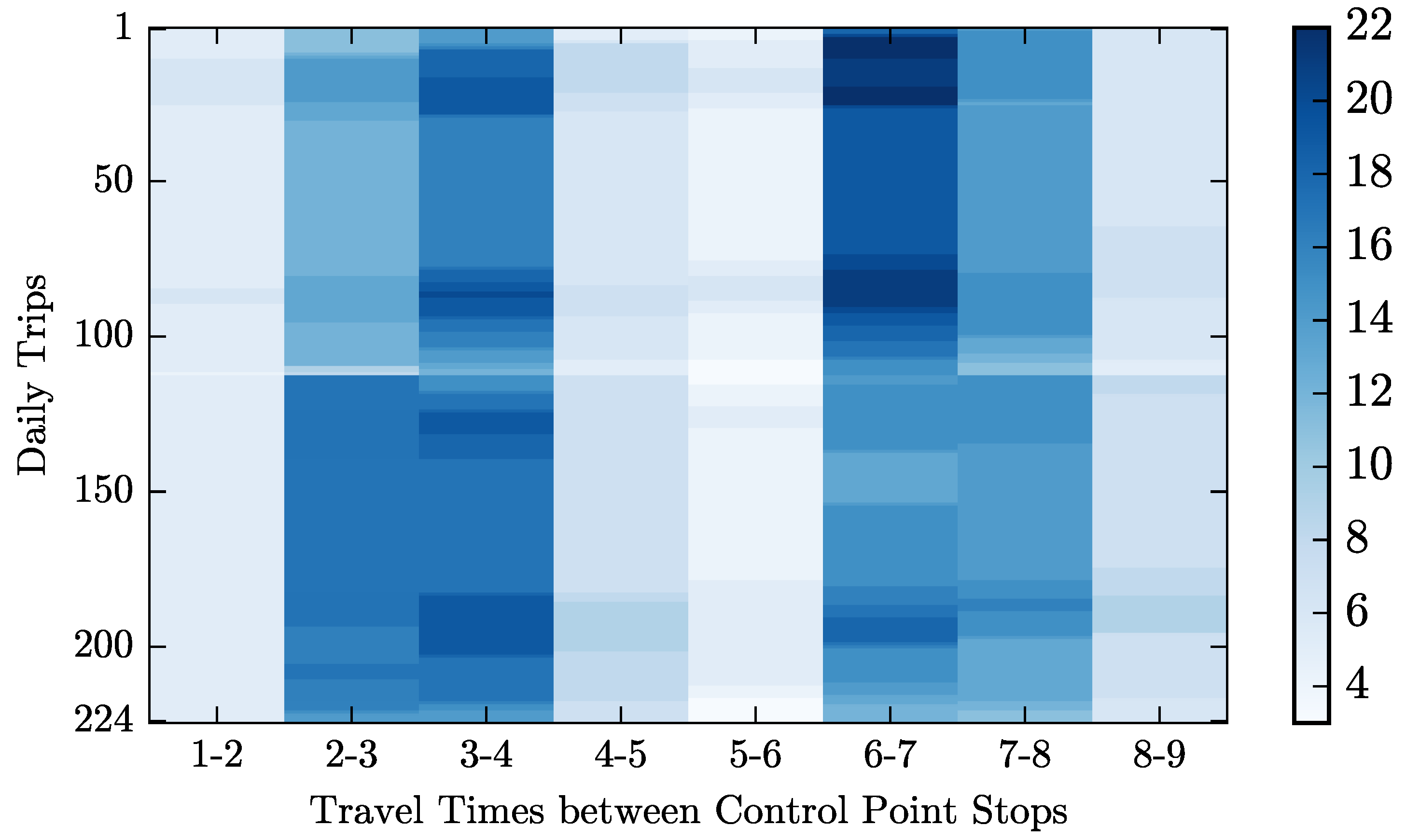
Figure 3.
Penalty function reduction at every iteration of the GA.
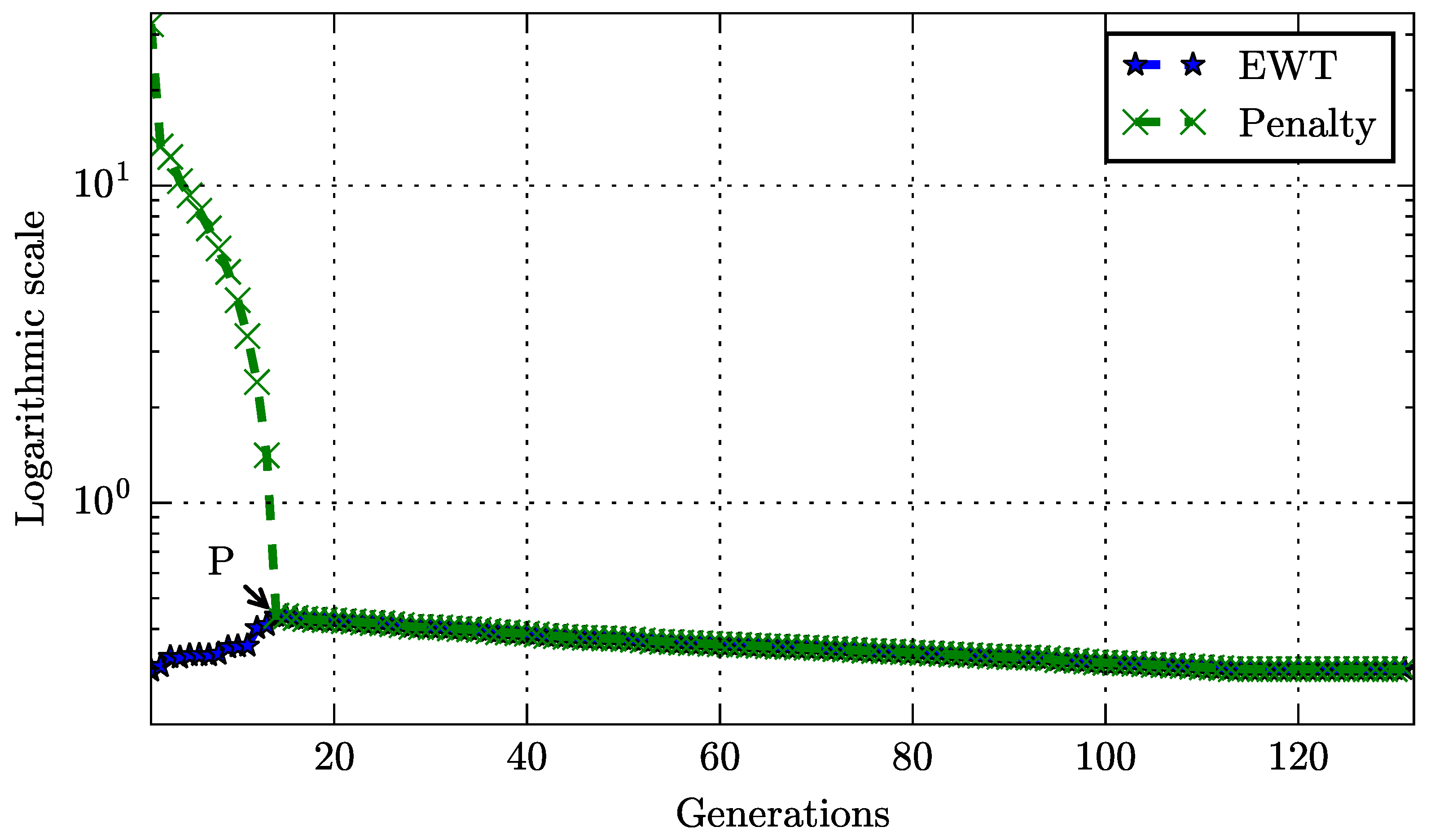
Figure 4.
Dispatching headways between consecutive trips of the initial random guess and the optimized timetable.
Figure 4.
Dispatching headways between consecutive trips of the initial random guess and the optimized timetable.

Figure 5.
Variation of constraints with every generation.
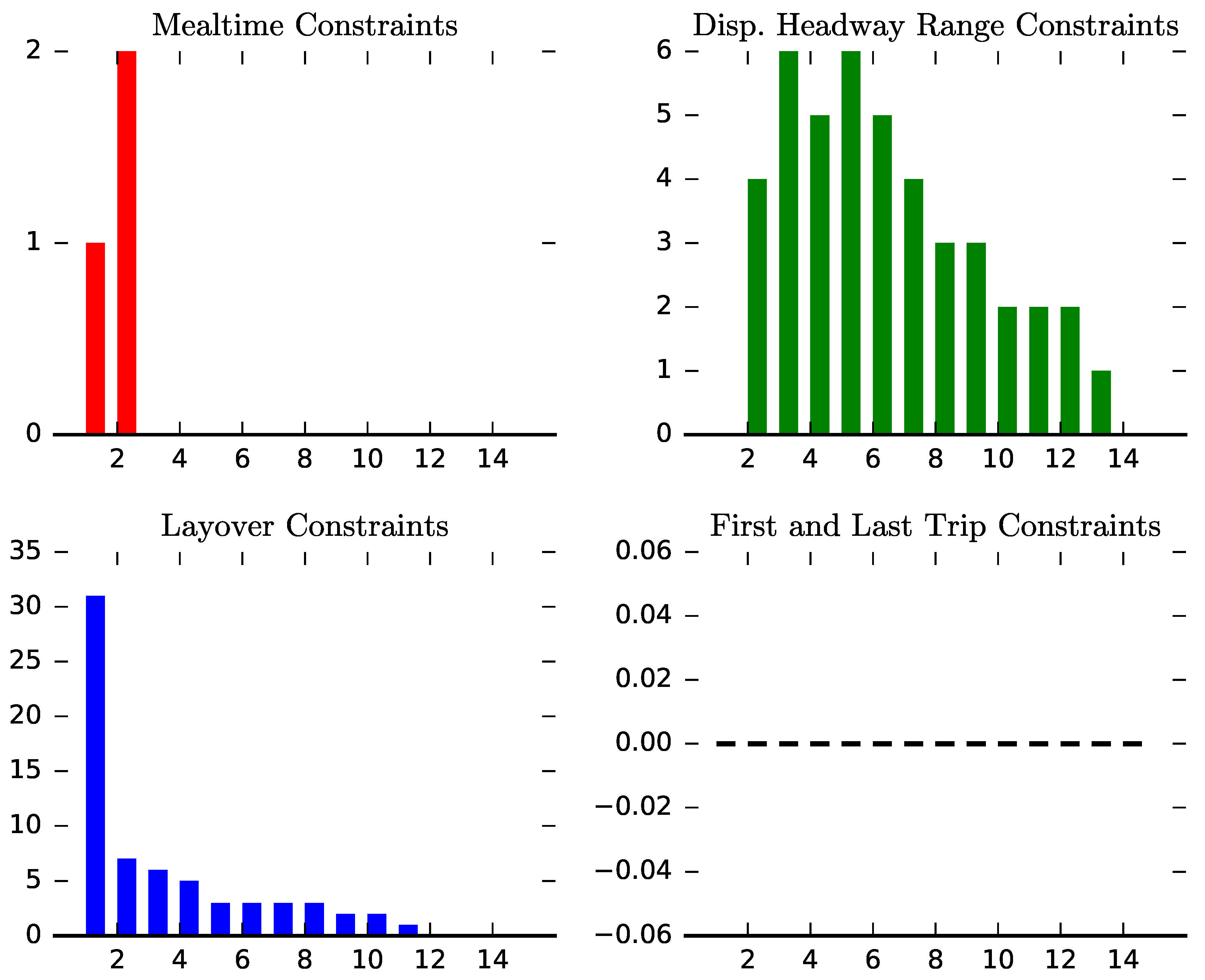
Figure 6.
Simulation output showing variation in violation of constraints.

Table 1.
Common Notations.
| Symbols | Description |
|---|---|
| D | Scheduled arrival time of each trip at each stop |
| N | Set of trips in the selected line for a day |
| S | Set of stops in the selected line |
| Upper limit of dispatching headways between consecutive trips | |
| Lower limit of dispatching headways between consecutive trips | |
| l | Allowed layover/Break time for each trip |
| m | Allowed mealtime break for every bus driver |
| start time of the first trip of the day | |
| start time of the last trip of the day | |
| k | typical dwell time at stops |
| estimated travel time of trip i between stops j and |
Table 2.
Lower and Upper Limits of Dispatching Headways between consecutive Trips for different Time Periods of the Day.
Table 2.
Lower and Upper Limits of Dispatching Headways between consecutive Trips for different Time Periods of the Day.
| Time Period (min.) | Direction 1 | Direction 2 |
|---|---|---|
| 390–510 | 6–10 min | 7–11 min |
| 510–1020 | 5–13 min | 7–13 min |
| 1020–1140 | 8–15 min | 7–9 min |
| 1140–1380 | 10–16 min | 9–15 min |
© 2018 by the authors. Licensee MDPI, Basel, Switzerland. This article is an open access article distributed under the terms and conditions of the Creative Commons Attribution (CC BY) license (http://creativecommons.org/licenses/by/4.0/).
Share and Cite
MDPI and ACS Style
Gkiotsalitis, K.; Kumar, R. Bus Operations Scheduling Subject to Resource Constraints Using Evolutionary Optimization. Informatics 2018, 5, 9. https://doi.org/10.3390/informatics5010009
AMA Style
Gkiotsalitis K, Kumar R. Bus Operations Scheduling Subject to Resource Constraints Using Evolutionary Optimization. Informatics. 2018; 5(1):9. https://doi.org/10.3390/informatics5010009
Chicago/Turabian StyleGkiotsalitis, Konstantinos, and Rahul Kumar. 2018. "Bus Operations Scheduling Subject to Resource Constraints Using Evolutionary Optimization" Informatics 5, no. 1: 9. https://doi.org/10.3390/informatics5010009
Note that from the first issue of 2016, this journal uses article numbers instead of page numbers. See further details here.