A Smart Sensor Data Transmission Technique for Logistics and Intelligent Transportation Systems


Department of Computer Science and Engineering, Kyung Hee University, 1732, Deogyeong-daero, Giheung-gu, Yongin-si 17104, Gyeonggi-do, Korea
*
Author to whom correspondence should be addressed.
Informatics 2018, 5(1), 15; https://doi.org/10.3390/informatics5010015
Submission received: 22 January 2018
/
Revised: 9 March 2018
/
Accepted: 13 March 2018
/
Published: 16 March 2018
(This article belongs to the Special Issue IoT and Informatics Applications in Logistics and Intelligent Transportation Systems)
Abstract
:When it comes to Internet of Things systems that include both a logistics system and an intelligent transportation system, a smart sensor is one of the key elements to collect useful information whenever and wherever necessary. This study proposes the Smart Sensor Node Group Management Medium Access Control Scheme designed to group smart sensor devices and collect data from them efficiently. The proposed scheme performs grouping of portable sensor devices connected to a system depending on the distance from the sink node and transmits data by setting different buffer thresholds to each group. This method reduces energy consumption of sensor devices located near the sink node and enhances the IoT system’s general energy efficiency. When a sensor device is moved and, thus, becomes unable to transmit data, it is allocated to a new group so that it can continue transmitting data to the sink node.
1. Introduction
City logistics is defined as the process for totally optimizing the logistics and transport activities by private companies with the support of advanced information systems in urban areas considering the traffic environment, its congestion, safety, and energy savings within the framework of a market economy [1]. Recently, robots have been developed and used in warehouse robots, self-driving trucks, transportation drones, and inland droids in the area of logistics. It is expected that in the future, these robots will be integrated systematically to realize autonomous logistics where every logistic activity including transportation and storage in and out of distribution centers will become automated and intelligent. As autonomous logistics are realized, city logistics will be operated using the organic exchange of information with an intelligent transportation system.
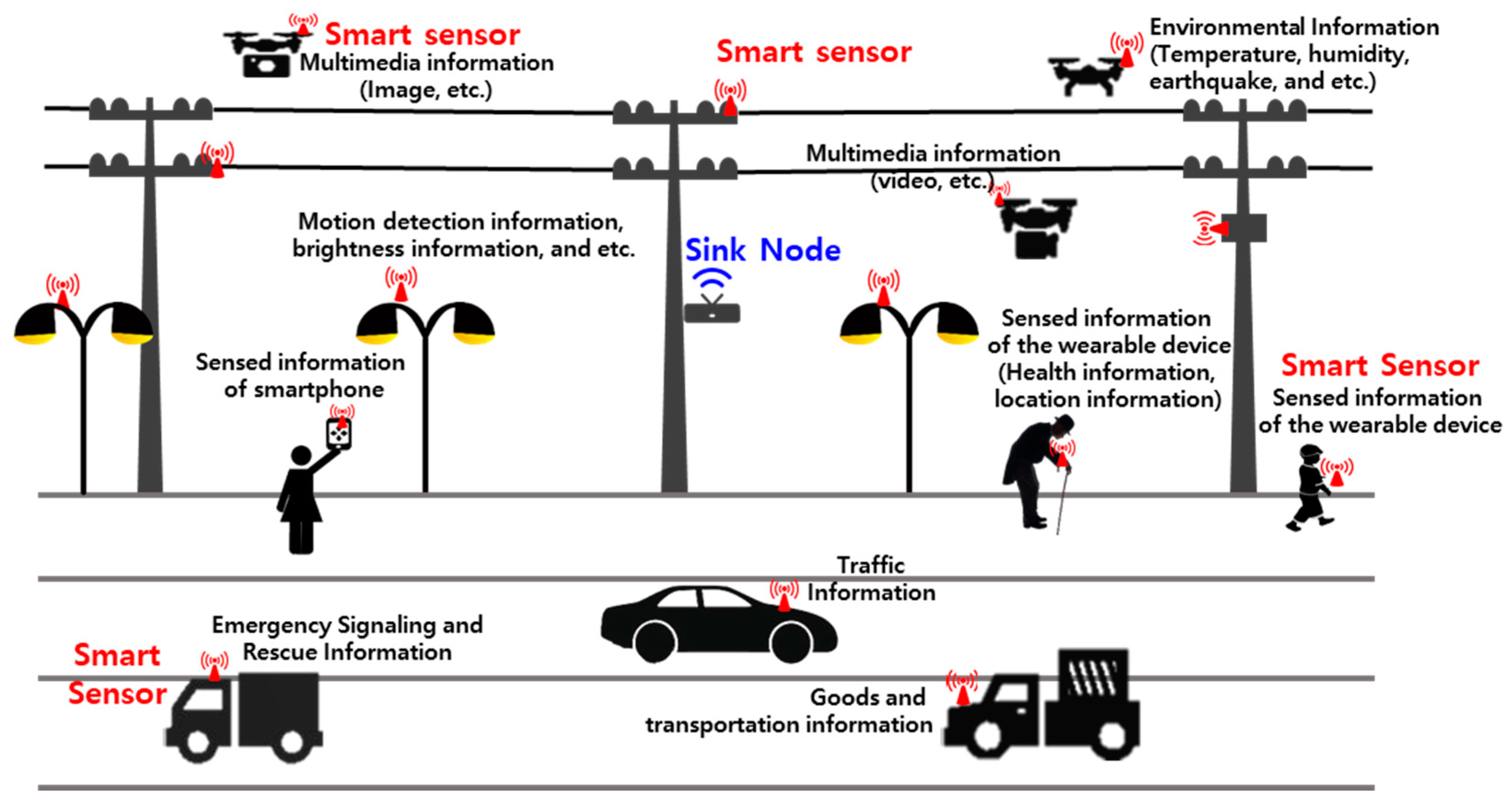
Components of city logistics and the intelligent transportation system such as robots, self-driving trucks, transportation drones, etc. collect various types of information including goods and delivery information, traffic information, safety and rescue information, Global Positioning System (GPS) and environmental information, etc. by means of smart sensors and then send such data via a wireless network. Figure 1 shows the concept of next-generation logistics and intelligent traffic information systems to which smart sensors and wireless networks are applied. Smart sensors are mounted on various components of the next-generation logistics and intelligent traffic information systems such as humans, smart phones, vehicles, and transportation drones to collect various types of data. As data are transmitted among smart sensors, a sink node collects all of the data and sends them to related systems via the Internet. Smart sensors are arranged in a three-dimensional (3D) space, moving along with humans, vehicles, etc. in order to collect data from them.
Smart sensors are intelligent sensors with outstanding data processing ability, memory functions, communication functions, independent power sources, etc. These sensors can provide users with every type of information necessary for applications, as well as general information basically required anywhere [2]. In order to improve the quality of life, smart sensors connect humans to things and help in the efficient resource management of industrial sites. Particularly, mobile smart sensor devices are one of the core elements of Internet of Things (IoT) systems that include next-generation logistics and an intelligent transportation information system. These devices can be utilized to acquire information from regions hardly approachable or dangerous due to topographical features for one.
In general, mobile smart sensor devices have a limited energy capacity. Once energy is entirely exhausted and the operation stops, the entire IoT system is affected. Thus, mobile sensor devices need to secure an energy life span for as long as possible. It should be possible to transmit data collected by the smart sensor devices of an IoT system to the sink node. For communication between mobile smart sensor devices, the Medium Access Control (MAC) layer controls access to shared wireless media and it is a major element that consumes energy. It is important, therefore, to design an efficient MAC protocol [3,4].
Mobile sensor devices of an IoT system may be arranged at random positions or distributed in areas that people find difficult to approach. Thus, these devices need to be autonomous to some extent [5]. As drones, including cameras, sensors, communication functions, etc. have been developed and used recently, mobile sensor devices can be positioned not only on the ground but also in the air. Thus, self-organizing is required not only on a two-dimensional (2D) plane but also in a 3D space so that the mobility of sensor devices can be supported.
Many studies have been conducted to enhance the energy efficiency of smart sensor nodes that are utilized in a sensor network. A major example is the ZigBee that is an IEEE 802.15.4-based specification for a suite of high-level communication protocols used to create personal area networks with small, low-power digital radios and other low-power, low-bandwidth needs, designed for small-scale projects which need wireless connections [6]. Unnecessary energy consumption may be reduced by avoiding collision, but the energy efficiency is not improved since the channel monitoring needs to continue. The approach stated in [7] utilizes the low-level carrier’s preamble sensing method in order to minimize energy consumption. This method is supposed to turn on or off the wireless communication device regularly. Wise MAC reduces energy consumption by adjusting the preamble length depending on network traffic [8]. S-MAC applies the concept of “time slot” in order to reduce energy consumption [9]. S-MAC uses a fixed duty cycle while T-MAC uses an adaptive duty cycle in order to enhance the energy efficiency [10]. E2-MAC adjusts the data transmission of a smart sensor node based on the concept of “buffer threshold” in order to improve the energy efficiency of T-MAC [11]. The PW-MAC protocol adds the pseudo-random number to a receiver’s beacon frame so that the sending node can predict the wake-up time of the receiving node [12]. XY-MAC applies the Early Termination method that minimizes the Early Acknowledge (ACK) section in order to reduce the idle listening time of the receiving node that may increase due to the sending node’s Early ACK section [13]. ODMAC proposes an energy-saving method that extends or shortens the beacon cycle in reflection of the energy consumption status of the smart sensor node on the assumption that in an energy harvesting environment, the network life span can be long unless there is any physical defect [14]. Dynamic S-MAC adjusts the frame length depending on the traffic status on the network in order to enhance S-MAC’s energy consumption [15]. EA-MAC adds the node correlation analysis algorithm and traffic-adaptive duty cycle mechanism to make up for the disadvantages of S-MAC [16]. Kim and Ryoo et al. [17,18] propose a method that maximizes the entire system’s energy life span in consideration of the fact that smart sensor nodes near the sink node consumes more energy than those far from it. Such MAC protocols are proposed mostly to enhance the energy efficiency of individual smart sensor devices but do not take into consideration of the mobility of the smart sensor devices of an IoT system, as well as the entire system’s energy life span.
The Sensor Node Group Management MAC (SGM-MAC) Scheme proposed in this study groups smart sensor nodes positioned for the Logistics and Intelligent Transportation System so that data can be transmitted only in the direction of that sink node. Each group is given a different buffer threshold when data are to be transmitted so that the energy consumption of smart sensor nodes near the sink node is reduced with the energy efficiency of the entire system enhanced. If a smart sensor node is relocated and deviates from the existing communication channel, a new group is designated so that it can continue sending data to the sink node. If the data collected by a smart sensor node is of urgency, it is given the top priority so that data transmission delay is prevented in the proposed method.
The rest of this study consists of the following sections: Section 2 specifies the energy-efficient data transmission method of the proposed SGM-MAC Scheme. Section 3 presents the details of the proposed method’s embodiment and performance evaluation results. Section 4 includes a summary of findings, and Section 5 is the conclusion of this study that presents the direction for future study.
2. SGM-MAC Scheme
2.1. Smart Sensor Node Grouping
The proposed method applies the T-MAC adaptive duty cycle that is designed to switch to the sleep mode if the smart sensor node fails to sense a transmission event for a certain period of time. It groups smart sensor nodes based on the communication distance between smart sensor nodes and the sink node.
2.1.1. Initial Group ID Setting
Initial Group ID setting means that the sink node sets the group ID of entire smart sensor nodes. In general, initial group ID setting is required when the sink node and smart sensor nodes are allotted to the system initially and when the sink node resets the group ID of the entire smart sensor nodes in that system. The sink node may reset the group ID of smart sensor nodes on a regular basis because more nodes are added to the system or some nodes are moved and become unable to transmit data. In such cases, resetting the group ID of the entire smart sensor nodes can reduce the general overhead of the system.
For initial group ID setting, the “Advertisement Packet” is used. The sink node generates the Advertisement Packet that includes its own group ID (the sink node’s group ID is 0) and the version information for initial group ID setting, and then this packet is transmitted to every smart sensor node around the sink node.
The process for initial group ID setting is as follows:
- (1)
- A sink node sets its group ID to 0 and generates advertisement packets that include the group and version information for group setting, sending the packets to every smart sensor node within a distance that allows transmission between them.
- (2)
- If a smart sensor node with no group ID setting receives advertisement packets, it adds 1 to the received group ID and sets the value as its group ID. Once the group setting version is renewed, an advertisement packet that includes these two sets of information is generated and transmitted to adjacent smart sensor nodes within the distance. The smart sensor node remembers its position in order to trace the track of its movement in the future.
- (3)
- If a smart sensor node with a group ID already receives advertisement packets, it checks whether its own version of information is an update of the received group setting version information. If the received information is new, it adds 1 to the received group ID and sets the value as its group ID. Once the group setting version is renewed, an advertisement packet that includes these two sets of information is generated and transmitted to adjacent smart sensor nodes within the distance. The smart sensor node remembers its position in order to trace the track of its movement in the future.
If the received group setting is older information, the received group ID is compared with its own group ID in order to check whether the advertisement packet has been received from the same group or from the downstream group.
Otherwise, its group ID is set by adding 1 to the received group ID value with the version of group setting renewed. An advertisement packet that includes these two sets of information is then generated and transmitted to adjacent smart sensor nodes within the distance. The smart sensor node remembers its position in order to trace the track of its movement in the future.
- (4)
- Steps 2 to 3 are repeated until the group ID is set for each of the smart sensor nodes.
Figure 2 shows the process that a smart sensor receives the Advertisement Packet and then resets the group ID.
Because the group ID is set with the value of the received group ID + 1 when the group ID of the sink node is 0, smart sensor nodes far from the sink node are given a larger group ID value. After the process in Figure 2 is completed for every smart sensor node in the system, the initial group ID setting is finalized.
2.1.2. Data Transmission Channel
Once the grouping process is completed, smart sensor nodes send data only to the nearest smart sensor node of the upper-level group. In other words, data transmission between smart sensor nodes is implemented always in the direction of the smart sensor node whose group ID is relatively small, and the data transmission channel up to the point of the sink node is of a tree structure.
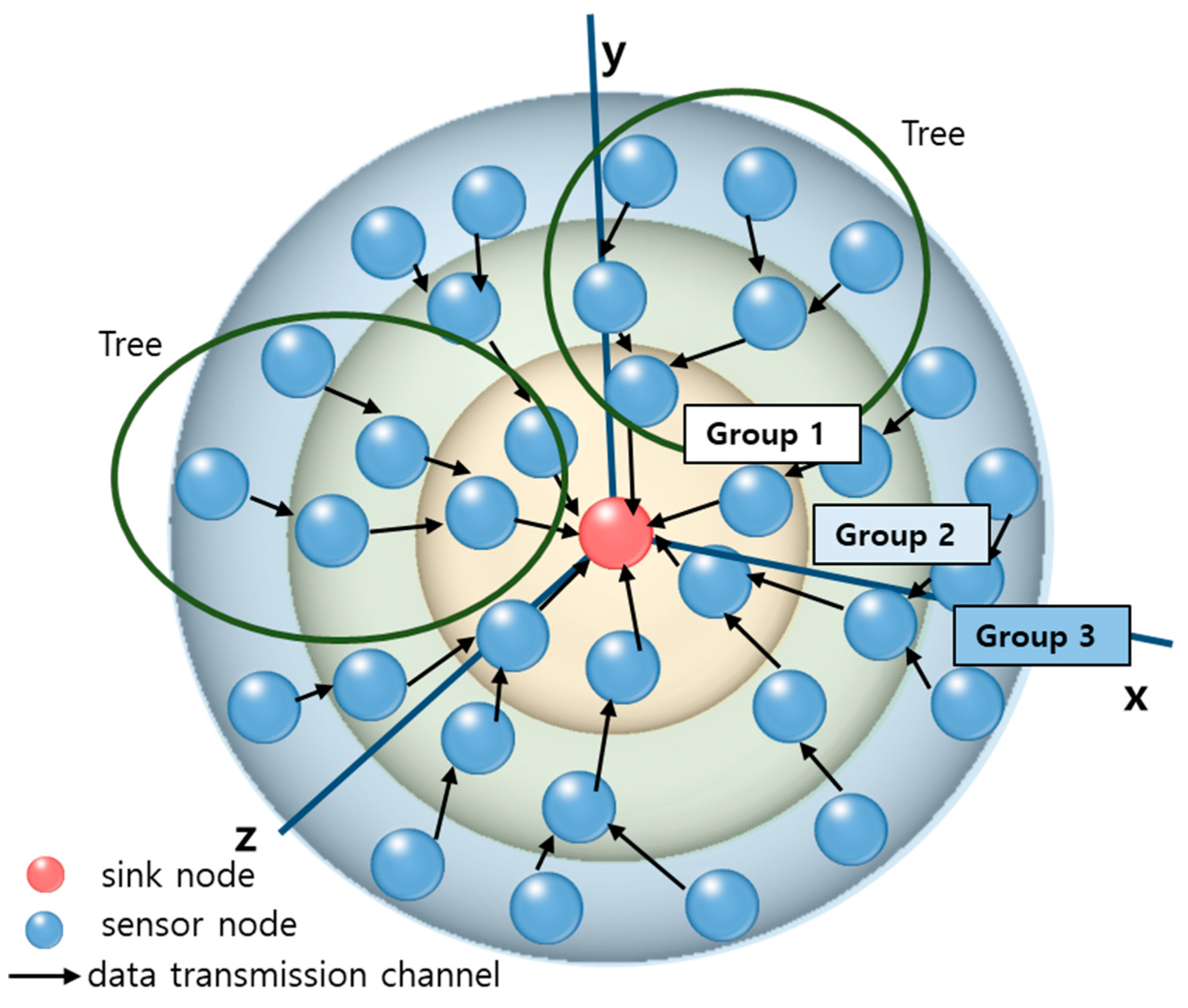
Figure 3 shows how the data of smart sensor nodes are transmitted only in the direction of the sink node. It shows that smart sensor nodes are arranged, centering the sink node in the 3D space. In the x axis, y axis, and z axis of the 3D space, it is assumed that the sink node is located at the position of (0.0.0), and each smart sensor node has its specific location value in the x axis, y axis, and z axis. This paper explains and simulates the concept of arranging sensor nodes in the three-dimensional space by means of the x, y, and z axes. In actual system, however, it is also possible to values sensor nodes’ latitude, longitude, and height above sea level values. When latitude, longitude, and height above sea level values are utilized, however, there might be some difference from the actual position and thus additional research is necessary to address this problem. When every sensor node is given a group ID, it is possible to group sensor nodes based on sink nodes. In Figure 3, the group ID of sensor nodes within the yellow circle is 1, that of sensor nodes within the green circle is 2, and that of sensor nodes within the blue circle is 3. Black arrows indicate that a sensor node sends data to the closest sensor node in the upper-level group. For example, a sensor node in Group 3 sends the closest sensor node belonging to Group 2. As the black arrows lead up to the sink node, the path of data transmission is indicated. The data transmission channel up to the sink node is of a tree-shaped structure. The dark green circle in Figure 3 shows an example of a data transmission channel of a tree-shaped structure.
Figure 4 shows the concept of data transmission between smart sensor nodes of different groups.
2.2. Support for Mobility of Smart Sensor Nodes
The proposed method supports the mobility of smart sensor nodes. When a smart sensor node is moved and becomes unable to send data, its group ID needs to be reset. This problem may be addressed through the regular initial group ID setting of the sink node, but as the interval is short, the overhead becomes significant accordingly. The proposed method resets the group ID when smart sensor nodes are in either of the two following cases:
- (1)
- When smart sensor nodes’ movement exceeds a certain distanceIn order to recognize when smart sensor nodes’ movement exceeds a certain distance, smart sensor nodes calculate the travel distance regularly in reference to its location data. As for the travel distance, the lineal distance from the position where each smart sensor node set its latest group ID to its current position is calculated. The “d” for the judgment that smart sensor nodes’ movement exceeds a certain distance may be illustrated with Formula (1) below:
- maxD: the maximum distance that sensor nodes can communicate with
Here, the maximum value of “d” indicates the maximum value of the distance in which smart sensor nodes can communicate with other nodes, and it may be varied depending on the weight “dw”. As the value of dw is close to 0, the procedure of group ID resetting is initiated when the smart sensor node moves regardless of the distance. Since the value of dw is close to 1, the group ID is reset only when the smart sensor node moves to a large degree. If the group ID is reset frequently, the overhead increases accordingly while the probability of data failure in smart sensor node movement decreases. If the group ID is reset only when the smart sensor node moves to a large degree, the overhead decreases but the time of data transmission failure upon smart sensor node movement is prolonged. As a result, the probability of data transfer delay increases. Therefore, the weight “dw” may be set differently by the system developer depending on the system to which smart sensor nodes are applied. - (2)
- Smart sensor node recognizing that it is unable to send data to the smart sensor node of the upper-level groupWhen smart sensor node sends Request To Send (RTS) three times to send data to the smart sensor node of the upper-level group but fails to receive Clear To Send (CTS), smart sensor node judges that it is no longer able to send data to the smart sensor node of upper-level group.
For group ID resetting of smart sensor nodes, the “Hello Packet” and the “Reply Packet” are used. Smart sensor nodes whose group ID is to be reset send the Hello Packet to smart sensor nodes nearby. When receiving the Hello Packet, smart sensor nodes send back the Reply Packet that includes their own group ID. If smart sensor nodes sending the Reply Packet have moved a long distance, the reliability of the group ID in the Reply Packet may be relatively low. Thus, smart sensor nodes that send the Reply Packet need to wait before sending back the Reply Packet for a time in proportion to the travel distance after receiving the Hello Packet so that smart sensor nodes resetting the group ID can receive the Reply Packet that includes the group ID of higher reliability first. In other words, smart sensor nodes that have moved the shortest distance can send the Reply Packet earlier than the others while nodes that have moved a far distance can send the Reply Packet later. As waiting time is allotted to smart sensor nodes prior to Reply Packet transmission, conflicts among Reply Packets can be minimized. Sometime after sending the Hello Packet, smart sensor nodes stop receiving the Reply Packet and reset their group ID based on the received group ID and the calculated reliability.
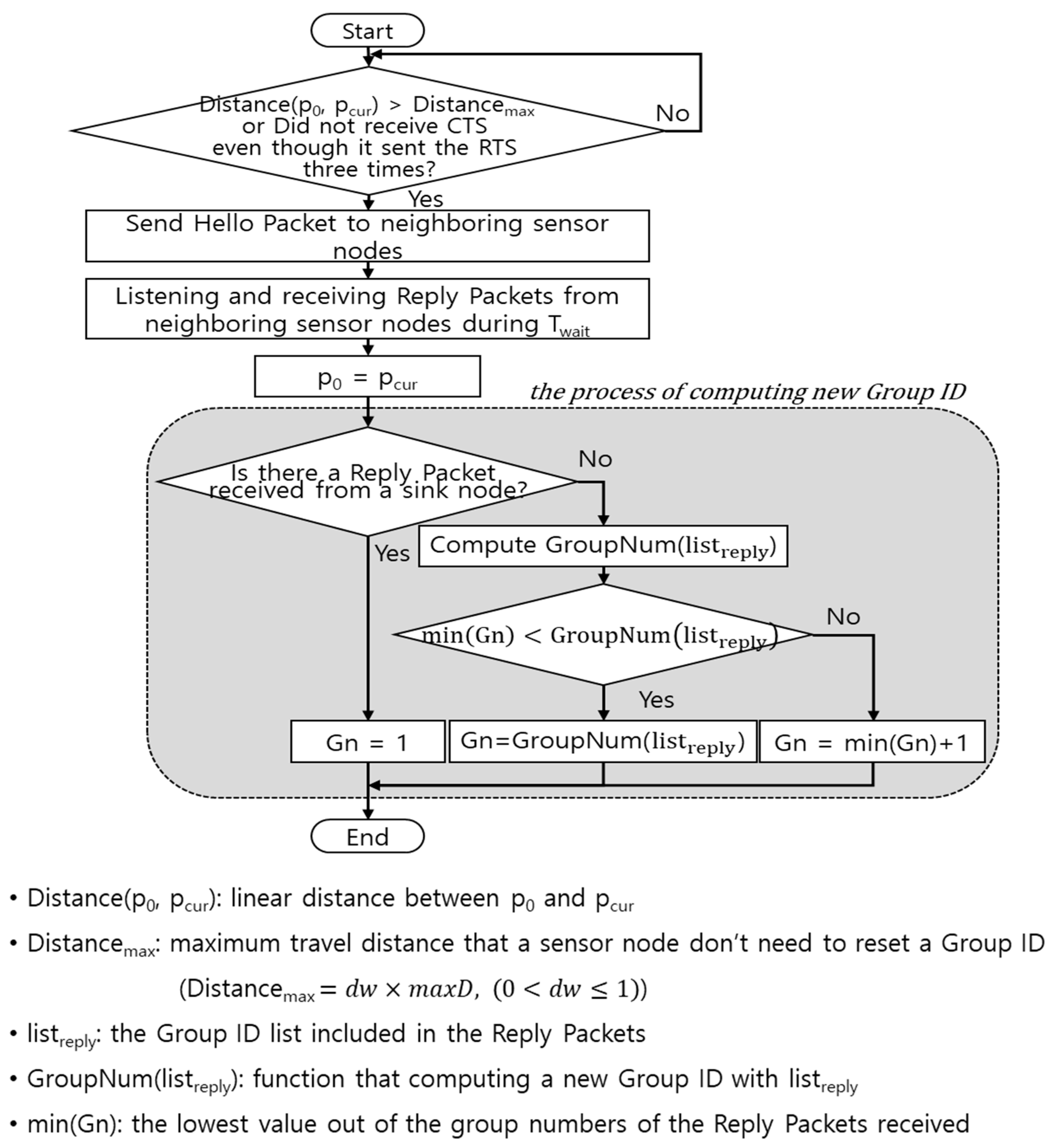
Figure 5 shows how smart sensor nodes trying to reset the group ID transmit the Hello Packet, receive the Reply Packet, and set a new group ID. When the Reply Packet has been received from the sink node, smart sensor nodes belong to group 1 and thus the group ID becomes 1. Otherwise, a new group ID is calculated by means of the GroupNum() function in reference to the group ID information in the Reply Packets received by smart sensor nodes. The GroupNum() function may be expressed with Formula (2) below. Since it is possible to send data only when the one-step upper level group exists within a distance where communication with smart sensor nodes is possible, the group ID value must be larger than the minimal value of the group IDs received from other adjacent nodes. Thus, if the value calculated by GroupNum() is larger than the minimal value of the group IDs in Reply Packets, a new group ID needs to be set based on the value of GroupNum(). Otherwise, the group ID becomes a value that is the minimal value of group IDs in the Reply Packet + 1.
Figure 6 shows the process that a smart sensor node receiving the Hello Packet transmits the Reply Packet. When a sink node receives a Hello packet, the smart sensor node that receives it should set the group ID to 1 and the sink node transmits a Reply packet. A smart sensor node that is not a sink node transmits a Reply packet after a time corresponding to the distance of its movement after receiving a Hello packet. In this manner, the smart sensor node that resets the group ID can receive a Reply packet including a group ID of high reliability earlier than others.
As shown in the GroupNum() function in Formula (2), rTime which is the weight for the travel distance of group IDs in each Reply Packet and gw which is the weight for group IDs are calculated to get the average group ID value. The resulting value is rounded off to the nearest integral number, and the integral number is designated based on the value as a new group ID. Smart sensor nodes that have traveled a long distance are likely to deviate from the group that they belonged to. Thus, a smaller weight is given to them. In general, smart sensor nodes adjacent to a smart sensor node are likely to be in lower-level group. Thus, group IDs of upper-level group are given a larger weight.
In Formula (3), the group weight gw may be varied depending on the system’s network environment. In general, the number of smart sensor nodes that belong to that group becomes larger as the group ID value increases. Thus, it is more accurate to apply a larger weight to a smaller group ID value when a group ID is calculated. Additionally, the number of smart sensor nodes that can be grouped together may be different depending on whether the nodes are arranged on a 2D plane or in a 3D space. The number of smart sensor nodes that can be arranged to each group is in proportion to the range (area or volume) of the group. When nodes are on a 2D plane, the area of a circle is applied; when they are in a 3D space, the area of a sphere is applied. The weight “gw” is calculated by substituting the area or volume of Group 1 with 1 and applying the reciprocal number of the area of volume for each group.
2.3. Buffer Threshold Setting
In the proposed method, the buffer threshold may be different depending on the group. The buffer threshold of smart sensor nodes that belong to a group far from the sink node (larger group ID value) is smaller than that of adjacent smart sensor nodes (smaller group ID value). In other words, the buffer threshold of smart sensor nodes in each group is in inverse proportion to the distance from the sink node. A smart sensor node saves its own data and data from other nodes in its buffer. When the data volume in the buffer is the same with or exceeds the buffer threshold, the data are transmitted to the most adjacent smart sensor node of the next higher-level group. Smart sensor nodes far from the sink node have more opportunities to send data to neighboring nodes than those near the sink node. In this manner, the proposed method maximizes the entire system’s energy efficiency.
The buffer threshold of smart sensor nodes may be decided by using Formula (4) below:
The buffer threshold formula suggested in this study can be applied generally. The buffer threshold may be different depending on the weight “bw” which may be set differently by the developer depending on system characteristics.
A smart sensor node collects data from smart sensor nodes that belong to a lower-level group and transmits it to smart sensor nodes of an upper-level group. Important variables to be considered when the buffer threshold is to be set include the group ID and the number of smart sensor nodes that belong to a lower-level group of smart sensor nodes. In the event that the buffer threshold decreases simply linearly when the group ID value increases with this condition neglected, the energy efficiency is insignificant according to the result of the simulation. Hence, the following section introduces several buffer threshold setting methods that have applied to the proposed MAC’s simulation.
The first method is applicable when the number of smart sensor nodes that belong to a lower level and the total number of smart sensor node in the system are known. In order to reflect the difference in buffer thresholds among groups, Formulas (5)–(7) below may be considered:
The second method calculates each group’s buffer threshold based on the maximum number of smart sensor nodes that can be arranged in the group (volume of the sphere). The buffer threshold’s weight “gw” is calculated by substituting the volume of Group 1 with 1 and applying the reciprocal number of the volume of each group. The buffer threshold may be calculated by using Formula (8) below:
2.4. Urgent Data Transmission
The proposed method may involve data transmission delay since data are transmitted based on the buffer threshold set differently for each group. If the data collected by a smart sensor node is of urgency, it is given the top priority so that data transmission delay is prevented. To classify urgent data from ordinary data, flag “Fu” is used. When the value of Fu is 0, it is recognized as ordinary data. In this case, when in the active mode, each smart sensor node compares the size of collected data in its buffer with the threshold of its buffer. Data are transmitted only when the size is the same with or exceeds the threshold value. When the value of Fu is 1, smart sensor nodes recognize the collected data as urgent and give a higher priority to it for urgent transmission.
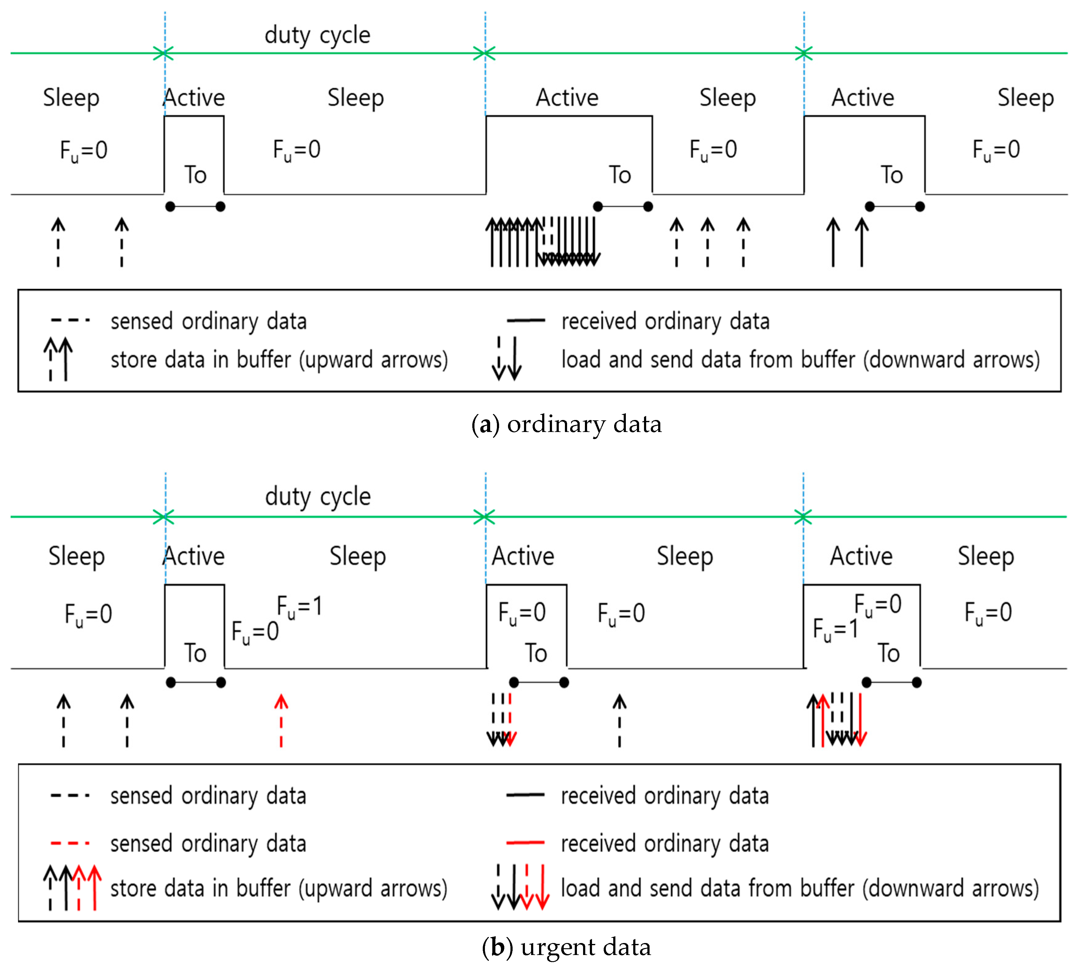
Figure 7a shows how to send ordinary data. It is assumed that the buffer threshold is set to the size of 8 data sets. A smart sensor node saves its own data and data from other nodes in its buffer. When the data volume in the buffer is the same with or exceeds the buffer threshold, the data are transmitted in the active mode to the most adjacent smart sensor node of the next higher level group. When the size of accumulated data is smaller than the buffer threshold, data may continue to be saved in the buffer or it may be switched to the sleep mode if no transmission event is sensed during a short time (To: Time out. This is the same with TA for the adaptive duty cycle of T-MAC [10]). As shown in Figure 7a, even if 2 sets of data sensed in the first active mode were saved in the buffer, the size of data was smaller than the buffer threshold. For this reason, the smart sensor node is converted into the sleep mode instead of transmitting the data. In the second active mode, 6 sets of data were received and saved in the buffer. As the size of data was larger than the buffer threshold, the data saved in the buffer are transmitted to the smart sensor node of an upper-level group. Since data are all ordinary data, the value of Fu is 0.
Figure 7b shows how to send urgent data. When there is a data set whose Fu value is 1 among collected data, the smart sensor node recognizes the data as urgent. In this case, the smart sensor node in the active mode sends all the data saved in the buffer regardless of the buffer threshold. As shown in Figure 7b, when the smart sensor node senses the first urgent data set, Fu is set to 1 and the urgent data are saved in the buffer. In the second active mode, three sets of data are saved in the buffer, and the size of data is smaller than the buffer threshold. However, the smart sensor node transmits all of the data in the buffer to the smart sensor node of an upper-level group, and the value of Fu is reset to 0. Likewise, as the data set received from the last active mode includes urgent data, the value of Fu is reset to 1, and the smart sensor node transmits all of the data immediately to the smart sensor node of an upper-level group regardless of the buffer threshold.
3. Results
3.1. Comparison of Smart Sensor Node Energy Consumption Depending on the Buffer Threshold
To compare the smart sensor node energy consumption of the proposed method depending on the buffer threshold, OPNET Modeler program was utilized. The simulation environments are assumed as in Table 1. When a smart sensor node moves, the group ID value or the number of smart sensor nodes of a lower-level group changes, and so does the buffer threshold. To compare the results, the mobility of smart sensor nodes was not considered in the simulation.
The simulated network topology is illustrated in Figure 8. To compare smart sensor nodes of various tree forms in the sub groups, 8 smart sensor nodes were selected randomly and their simulation results were compared. In Figure 8, the selected nodes are given numbers from 1 to 8. Nodes No. 1 and 2 belong to group 1 and are of a lower-level group. They have a tree of a different shape. The number of their lower-level nodes is 11 and 8, respectively. The group ID of nodes No. 3 and 4 is 2. The number of their lower-level nodes is 6 and 2 respectively. Nodes No. 5, 6, and 8 belong to group 3, and the number of their lower-level nodes is 2, 2, and 3 respectively. The group ID of Node No. 7 is 4, and it has 1 lower-level node.
3.1.1. Comparison of the Fixed Buffer Threshold and Variable Buffer Threshold
When every smart sensor node uses the fixed buffer threshold regardless of the group ID and when variable buffer thresholds are used depending on the group ID, the energy consumption of smart sensor nodes over time may be different as shown in Figure 9. The variable buffer threshold was calculated by applying Formula (6), and it was assumed that data were transmitted from each smart sensor node to the sink node at intervals of 15 min.
As shown in the simulation result, compared with the smart sensor node energy consumption when the fixed buffer threshold was applied regardless of the group ID, the energy consumption when the variable buffer threshold was applied depending on the group ID was more uniform.
Figure 9 shows the level of the energy consumption of smart sensor nodes near the sink node is higher than that of smart sensor nodes far from the sink node. When the sensor nodes near the sink node run out of energy, the data cannot be transmitted to the sink node. The energy consumption of smart sensor nodes near the sink node affects the energy life span of the entire system. In Figure 9b, energy consumption was uniform among smart sensor nodes regardless of the group ID. In Figure 9c, the mean of energy consumption was low among smart sensor nodes because the level of the energy consumption of smart sensor nodes far from the sink node is low when the fixed buffer threshold was applied. But, standard deviation of energy consumption was high among smart sensor nodes. On the other hand, the mean of energy consumption was high among smart sensor nodes because the level of the energy consumption of smart sensor nodes was uniform when the variable buffer threshold was applied. Standard deviation of energy consumption was low among smart sensor nodes. As shown in the simulation result, compared with the smart sensor node energy consumption when the fixed buffer threshold was applied regardless of the group ID, the energy consumption when the variable buffer threshold was applied depending on the group ID was more uniform. The fact that energy consumption was uniform among smart sensor nodes indicates that the energy consumption of certain smart sensor nodes does not affect the energy life span of the entire system. In other words, the energy life span of the entire system is improved.
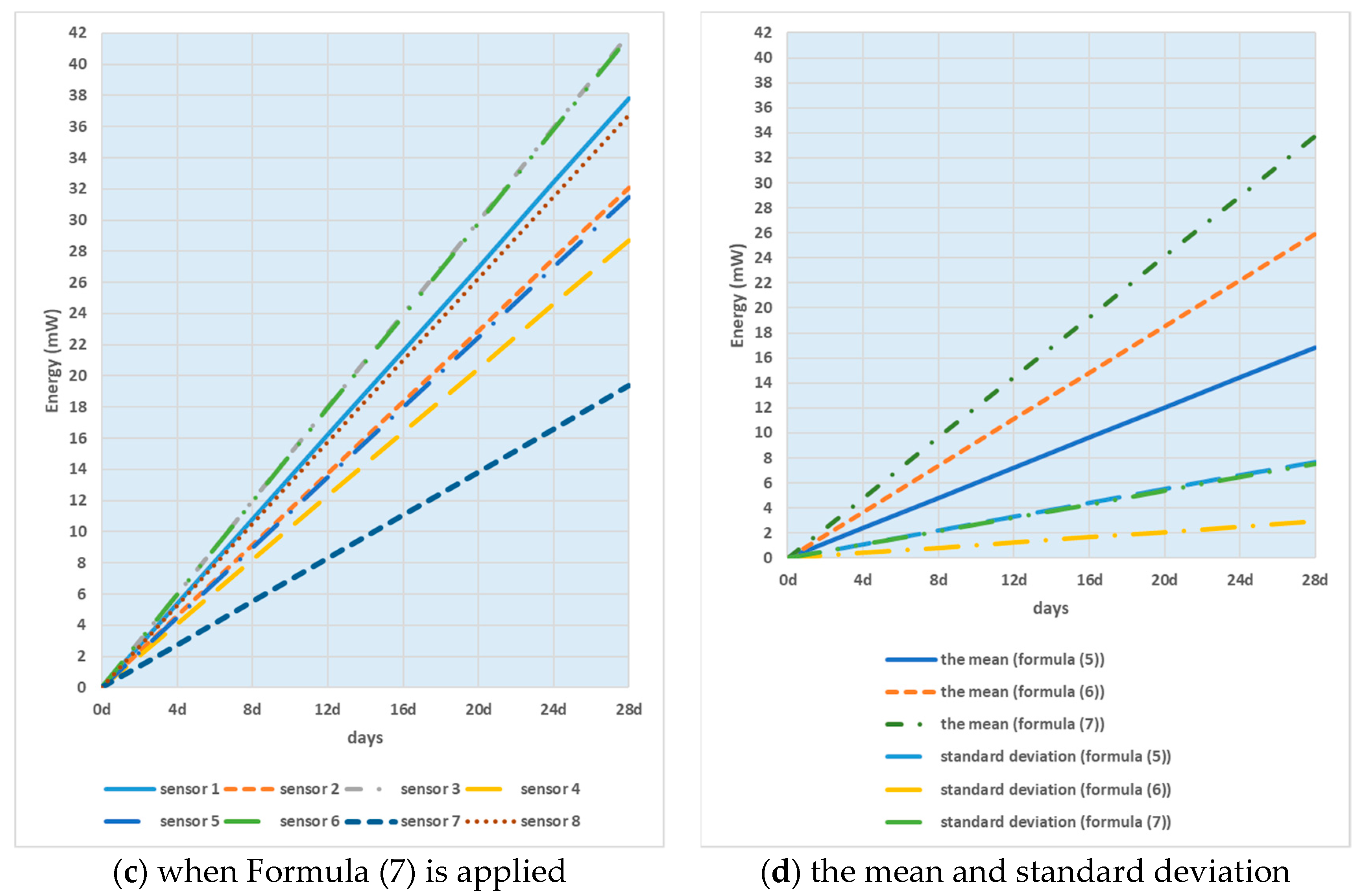
3.1.2. Comparison of Different Variable Buffer Thresholds
Figure 10 shows smart sensor node energy consumption when the variable buffer threshold was applied depending on each group ID. Formulas (5)–(7) were used.
Figure 10a shows that energy consumption was not uniform among smart sensor nodes because the buffer threshold difference between groups was not significant enough when the buffer threshold setting Formula (5) was applied. In Figure 10b to which the buffer threshold setting Formula (6) was applied, energy consumption was most uniform among smart sensor nodes. In Figure 10c to which the buffer threshold setting Formula (7) was applied, the level of energy consumption was higher among smart sensor nodes far from the sink node than that of smart sensor nodes near the sink node. This indicates that the buffer threshold difference between groups was excessive. In Figure 10d, standard deviation of energy consumption was the most lower among smart sensor nodes when the buffer threshold to which Formula (6) was applied. That is, the buffer threshold to which Formula (6) was applied led to the highest energy efficiency. It is important to set the optimal buffer threshold depending on the characteristics of the system where smart sensor nodes are distributed.
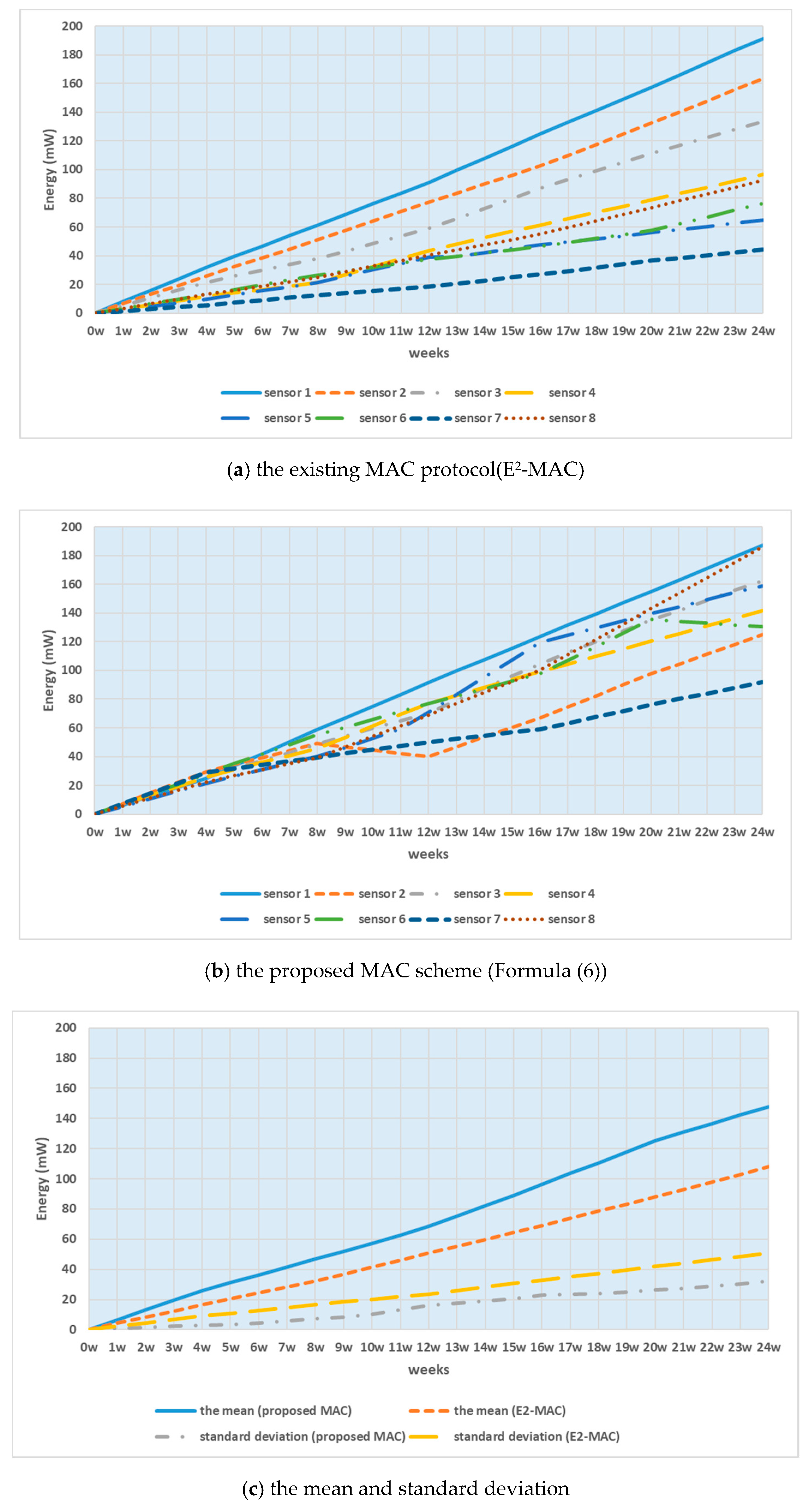
3.1.3. Comparison of the Existing MAC Protocol That Applies Fixed Buffer Thresholds and the Proposed MAC Protocol
Figure 11 compares the smart sensor node energy consumption of the existing MAC protocol that applies fixed buffer thresholds and the proposed method that applies variable buffer thresholds. The existing MAC protocol is E2-MAC. The simulated network topology seems to be similar, but the most significant difference from the proposed method is that the buffer threshold is fixed for each smart sensor node, and that smart sensor nodes are not grouped.
Figure 11a shows the smart sensor node energy consumption of the existing MAC protocol to which fixed buffer thresholds are applied. Figure 11b shows the smart sensor node energy consumption of the proposed method that applies variable buffer thresholds. In Figure 11c, the mean of energy consumption was low among smart sensor nodes of the existing MAC protocol. But, standard deviation of energy consumption was high among smart sensor nodes. On the other hand, the mean of energy consumption was high among smart sensor nodes of the proposed MAC scheme. Standard deviation of energy consumption was low among smart sensor nodes. The simulation result indicates that the energy consumption among smart sensor nodes of the proposed method is uniform in comparison with that of the existing MAC protocol.
3.2. Comparison of Energy Efficiency of Smart Sensor Nodes Moving in a 3D Space
C++ was utilized to realize the proposed method. The simulation environment is as shown in Table 2.
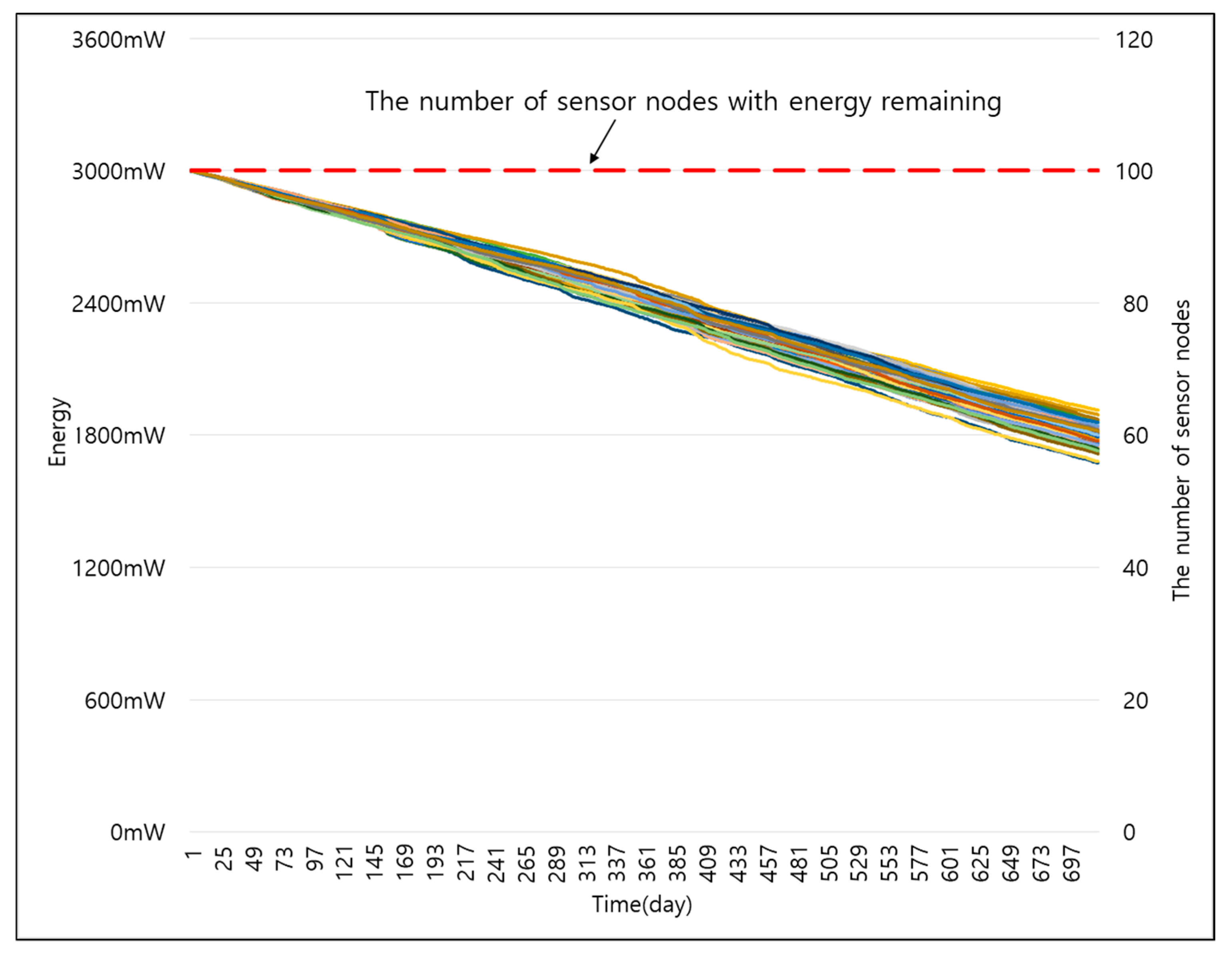
To verify the energy efficiency of the proposed method, the energy consumption of smart sensor nodes was compared with different sizes of data applied. Figure 12 shows the energy consumption of smart sensor nodes over time when the size of data was 1 byte (B). The energy consumption of smart sensor nodes decreased over time at a similar rate.
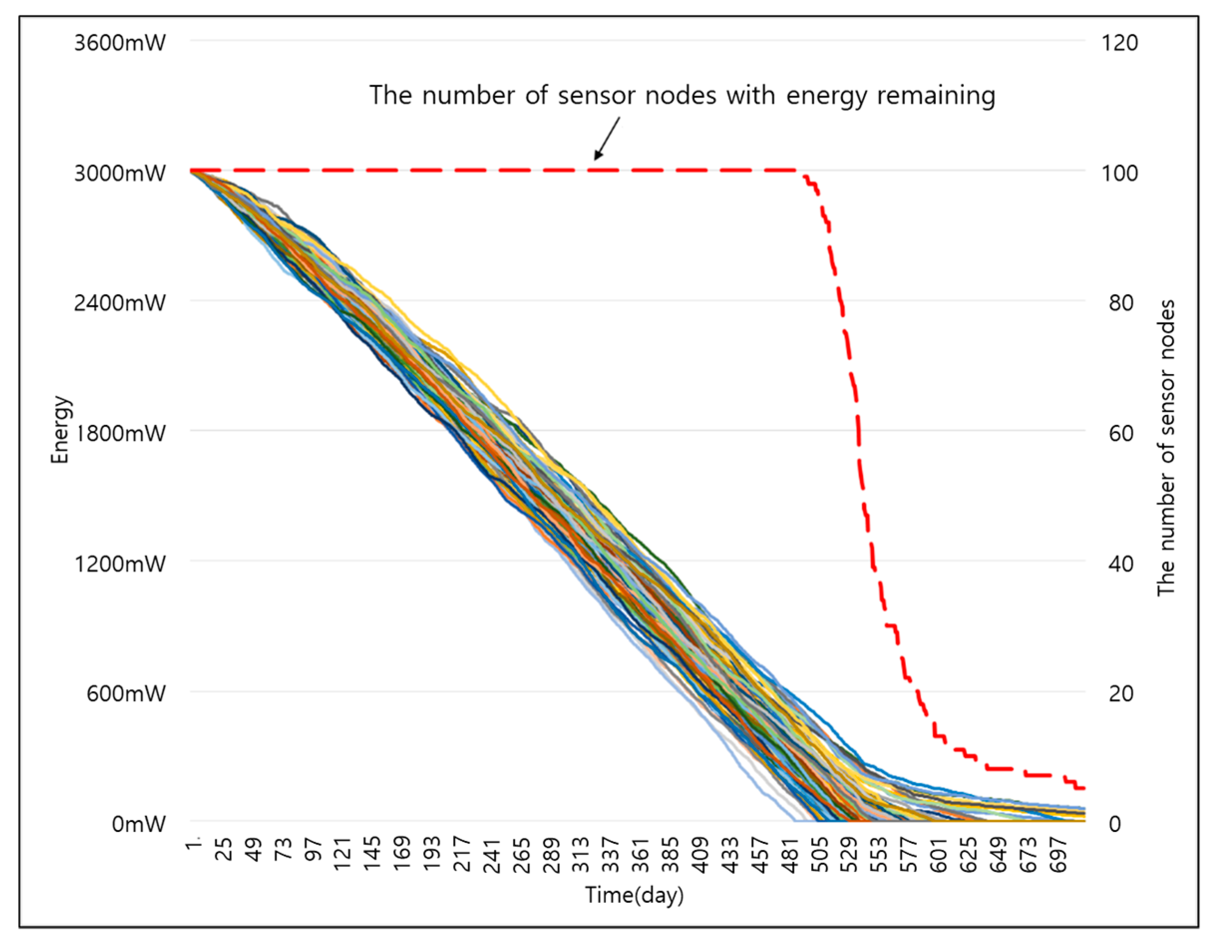
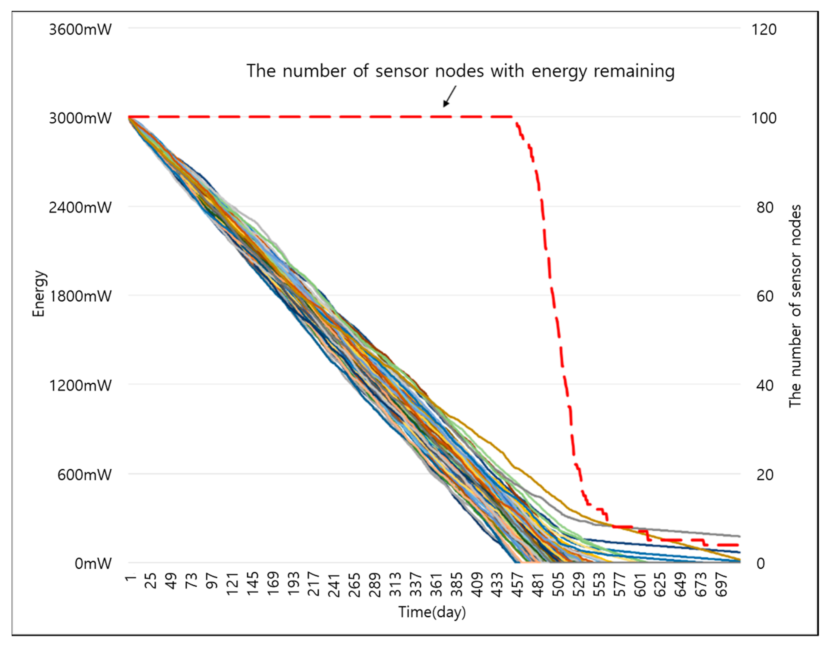
Figure 13 shows the energy consumption of smart sensor nodes over time when the size of data was 10 B. The energy consumption of smart sensor nodes decreased over time at a similar rate, and most smart sensor nodes ran out of energy at a similar timing. Since the data were relatively large and the number of data transmissions increased, energy consumption of smart sensor nodes was accelerated. However, the fact that most smart sensor nodes ran out of energy at a similar timing indicates that the energy consumption of certain smart sensor nodes does not affect the energy life span of the entire system. In other words, the energy life span of the entire system is maximized.
3.3. Comparison of the Average Transmission Duration of Ordinary Data and Urgent Data
In order to verify that smart sensor nodes could handle urgent data with no transmission delay in the proposed method, the average duration of data transmission from the smart sensor nodes of each group to the sink node was compared. With data of various sizes classified to ordinary and urgent data sets, the average duration of data transmission from smart sensor nodes (Groups 1–4) to the sink node was measured.
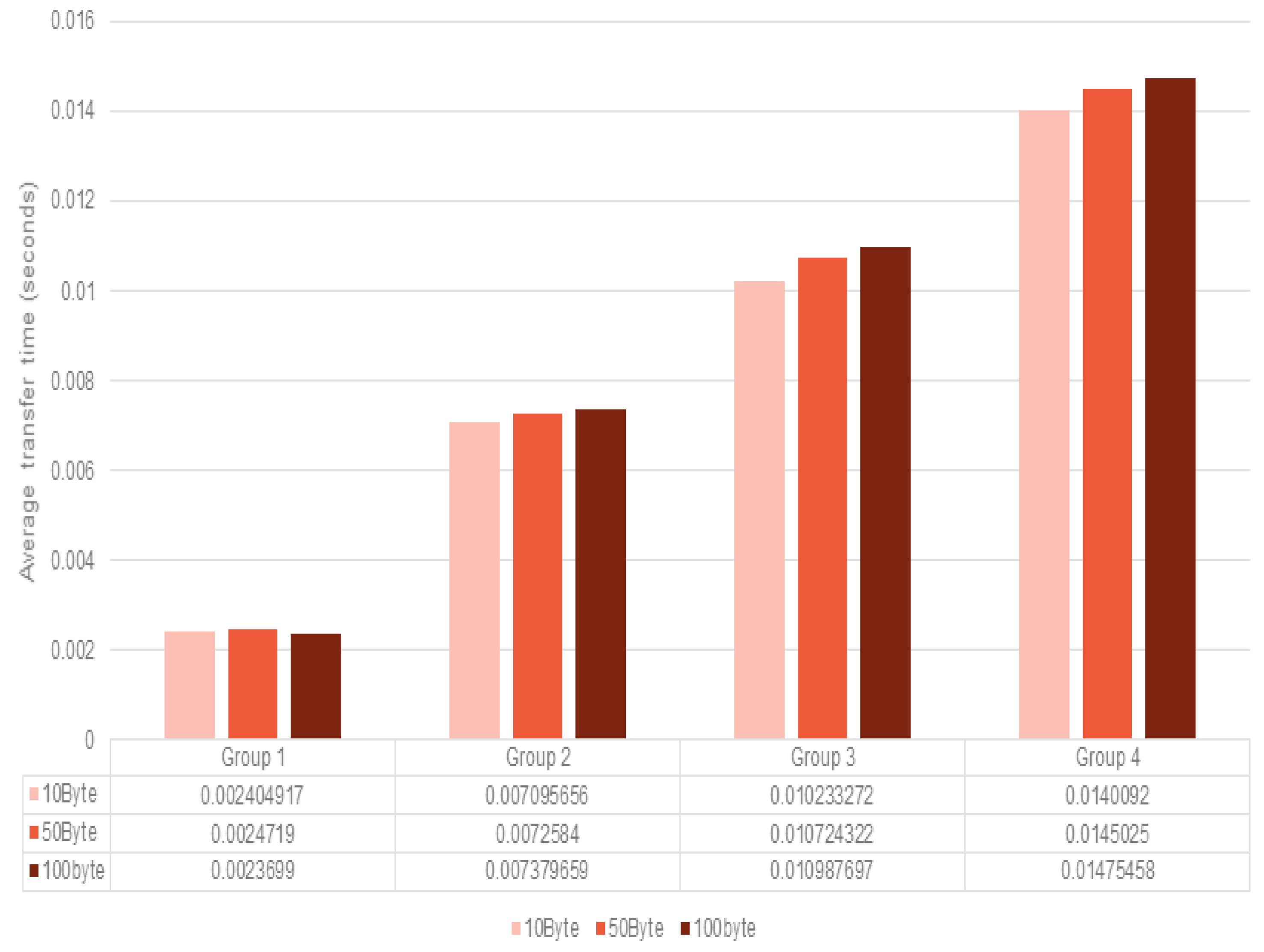
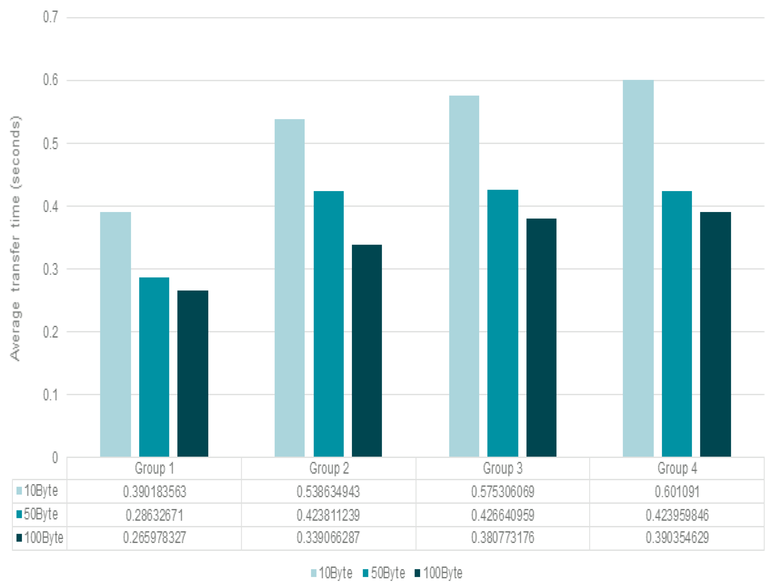
Figure 16 shows the average duration of ordinary data transmission by smart sensor nodes of each group depending on the data size. As the Group ID value was small, the duration of ordinary data transmission by smart sensor nodes was relatively short. As the size of data was large, the average data transmission time was short. Since different variable buffer thresholds are set for each smart sensor node group, the time to reach the buffer threshold is shortened as the data size is large and the group ID value is large.
Figure 17 shows the average duration of urgent data transmission by smart sensor nodes of each group depending on the data size. Urgent data is transmitted in the active mode immediately regardless of the buffer threshold setting of smart sensor nodes. Hence, the data size does not affect the data transmission time. Smart sensor nodes of a large group ID value send data to the sink node by a way of delivering data to a higher-level smart sensor node group. Thus, it takes more time for smart sensor nodes of a larger group ID value to send urgent data.
4. Discussion
In view of the simulation results, the proposed MAC scheme has demonstrated the following characteristics:
First, even if data were transmitted with different buffer thresholds applied to each group and thus the data sizes were varied, the proposed method adjusted the energy consumption of smart sensor nodes uniformly and enhanced the energy efficiency of the entire system as all of the smart sensor nodes ran out of energy at a similar timing. The future study needs to set clear standards for buffer thresholds and develop numerical formulas to calculate the optimal buffer threshold in consideration of various system environments.
Second, the system’s smart sensor nodes are grouped depending on the distance (hop) from the sink node. When it becomes impossible for certain smart sensor nodes to send data to the next-level group due to their movement, a new group ID is designated so that the nodes can continue sending data through a new channel properly. The future study needs to improve the numerical formulas for group ID resetting based on the criteria for the travel distance of smart sensor nodes and various system environments.
Third, the proposed method handled urgent data with no transmission delay. The future study needs to examine ways of prioritizing various urgent data sets and transmitting them based on the priorities.
5. Conclusions
This study proposed an MAC scheme that was designed to set group IDs to smart sensor nodes installed on mobile warehouse robots, self-driving trucks, transportation drones, etc. arranged for the Logistics and Intelligent Transportation System in a 3D space based on the distance of such nodes from the sink node. This proposed method also sent data based on the buffer thresholds designated in advance for each group in order to make full use of the limited battery capacity of smart sensor nodes.
The proposed method makes each smart sensor node send data in the direction of the sink node by means of group IDs. When certain smart sensor nodes are moved and become unable to send data to the next-level group, they are given a new group ID so that they can continue sending data through a new channel. Additionally, this method maximizes the system’s general energy life span by reducing the number of data transmissions of smart sensor nodes near the sink node in application of variable length buffer thresholds. When the data collected by smart sensor nodes are a type of urgent data, they are given a high priority so that the data can be delivered with no transmission delay.
Finally, the proposed MAC scheme has been proven to be energy-efficient through the performance test.
In the future, the criteria for the travel distance and criteria for buffer thresholds are to be established for the proposed MAC scheme. The numerical formulas for group ID resetting need to be improved in reflection of various system environments. Specific performance evaluation methods and routing or database management policies also need to be developed in order to advance the MAC protocol design to a higher level.
Acknowledgments
This research was supported by Korea Electric Power Corporation. (Grant number: R18XA02).
Author Contributions
The research is performed by Kyunghee Sun under the supervision of Intae Ryoo. Kyunghee Sun: main writing, design of the overall scheme, analysis, and improvement of the proposed scheme; Intae Ryoo: overall supervision of design of the scheme, analysis, paperwork, review, comments, etc.
Conflicts of Interest
The authors declare no conflict of interest.
References
- Taniguchi, E.; Thompson, R.G.; Yamada, T. Recent advances in modelling city logistics. In City Logistics II; Institute of Systems Science Research: Kyoto, Japan, 2001; pp. 3–33. [Google Scholar]
- Hunter, G.W.; Stetter, J.R.; Hesketh, P.; Liu, C.-C. Smart Sensor Systems. Electrochem. Soc. Interface 2010, 19, 29–34. [Google Scholar] [CrossRef]
- IEEE Std. 802.11-2012, IEEE Standard for Information Technology-Telecommunications and Information Exchange between Systems Local and Metropolitan Area Networks-Specific Requirements Part 11: Wireless LAN Medium Access Control (MAC) and Physical Layer (PHY) Specifications; IEEE: Piscataway, NJ, USA, 2012. [Google Scholar]
- Huang, P.; Xiao, L.; Soltani, S.; Mutka, M.W.; Xi, N. The Evolution of MAC Protocols in Wireless Sensor Networks: A survey. IEEE Commun. Surv. Tutor. 2013, 15, 101–120. [Google Scholar] [CrossRef]
- Sohrab, K.; Gao, J.; Ailawadhi, V.; Pottie, G.J. Protocol for Self-Organization of a Wireless Sensor Network. IEEE Pers. Commun. 2000, 7, 16–27. [Google Scholar] [CrossRef]
- ZigBee Alliance. ZigBee Specification, 2012, ZigBee Document 053474r20; ZigBee Alliance: Davis, CA, USA, 2012. [Google Scholar]
- El-Hoiydi, A. Aloha with preamble sampling for sporadic traffic in ad hoc wireless sensor networks. In Proceedings of the 2002 IEEE International Conference on Communications, ICC 2002, New York, NY, USA, 28 April–2 May 2002. [Google Scholar]
- El-Hoiydi, A.; Decotignie, D.; Enz, C.; LeRoux, E. Poster abstract: WiseMAC, an Ultra Low Power MAC protocol for the WiseNet wireless sensor network. In Proceedings of the 1st International Conference on Embedded Networked Sensor Systems, SenSys 03, Los Angeles, CA, USA, 5–7 November 2003; pp. 685–692. [Google Scholar]
- Ye, W.; Heidemann, H.; Estrin, D. An energy-efficient MAC protocol for wireless sensor networks. In Proceedings of the Twenty-First Annual Joint Conference of the IEEE Computer and Communications Societies, INFOCOM 2002, New York, NY, USA, 23–27 June 2002; IEEE: Piscataway, NJ, USA, 2002; Volume 3, pp. 1567–1576. [Google Scholar]
- Dam, T.V.; Langendoen, K. An adaptive energy-efficient MAC protocol for wireless sensor networks. In Proceedings of the 1st International Conference on Embedded Networked Sensor Systems, ACM SenSys ’03, Los Angeles, CA, USA, 5–7 November 2003; pp. 171–180. [Google Scholar]
- Kim, J.H.; Kim, H.N.; Kim, S.G.; Choi, S.J.; Lee, J.Y. Advanced MAC protocol with energy-efficiency for wireless sensor networks. In Proceedings of the International Conference on Information Networking: Convergence in Broadband and Mobile Networking, ICOIN 2005, Jeju Island, Korea, 31 January–2 February 2005; pp. 283–292. [Google Scholar]
- Tang, L.; Su, Y.; Gurewitz, O.; Johnson, D.B. PW-MAC: An energy-efficient predictive-wakeup MAC protocol for wireless sensor networks. In Proceedings of the INFOCOM 2011, Shanghai, China, 10–15 April 2011; pp. 1305–1313. [Google Scholar]
- Lu, Z.; Luo, T.; Wang, X. XY-MAC: A short preamble MAC with sharpened pauses for wireless sensor networks. In Proceedings of the 2012 IEEE Wireless Communications and Networking Conference (WCNC), Paris, France, 1–4 April 2012; pp. 1550–1554. [Google Scholar]
- Fafoutis, X.; Dragoni, N. ODMAC: An on-demand MAC protocol for energy harvesting—Wireless sensor networks. In Proceedings of the 8th ACM Symposium on Performance Evaluation of Wireless ad hoc, Sensor, and Ubiquitous Networks, ACM PE-WASUN ‘11, Miami, FL, USA, 3–4 November 2011; pp. 49–56. [Google Scholar]
- Yoo, D.S.; Choi, S.S. Medium Access Control with Dynamic Frame Length in Wireless Sensor Networks. J. Inf. Process. Syst. 2010, 6, 501–510. [Google Scholar] [CrossRef]
- Xu, D.; Wang, K. An adaptive traffic MAC protocol based on correlation of nodes. EURASIP J. Wirel. Commun. Netw. 2015, 2015, 258. [Google Scholar] [CrossRef]
- Kim, S.H.; Joh, H.G.; Choi, S.J.; Ryoo, I.T. Energy Efficient MAC Scheme for Wireless Sensor Networks with High-Dimensional Data Aggregate. Math. Probl. Eng. 2015, 2015, 803834. [Google Scholar] [CrossRef]
- Ryoo, I.T.; Sun, K.H.; Lee, J.S.; Kim, S.H. A 3-dimensional group management MAC scheme for mobile IoT devices in wireless sensor networks. J. Ambient Intell. Humaniz. Comput. 2017, 8, 1–12. [Google Scholar] [CrossRef]
Figure 1.
The concept of the next-generation logistics and intelligent transportation information system to which smart sensors and wireless networks are applied.
Figure 1.
The concept of the next-generation logistics and intelligent transportation information system to which smart sensors and wireless networks are applied.

Figure 2.
The process where a smart sensor receives the Advertisement Packet and then resets the group ID.
Figure 2.
The process where a smart sensor receives the Advertisement Packet and then resets the group ID.
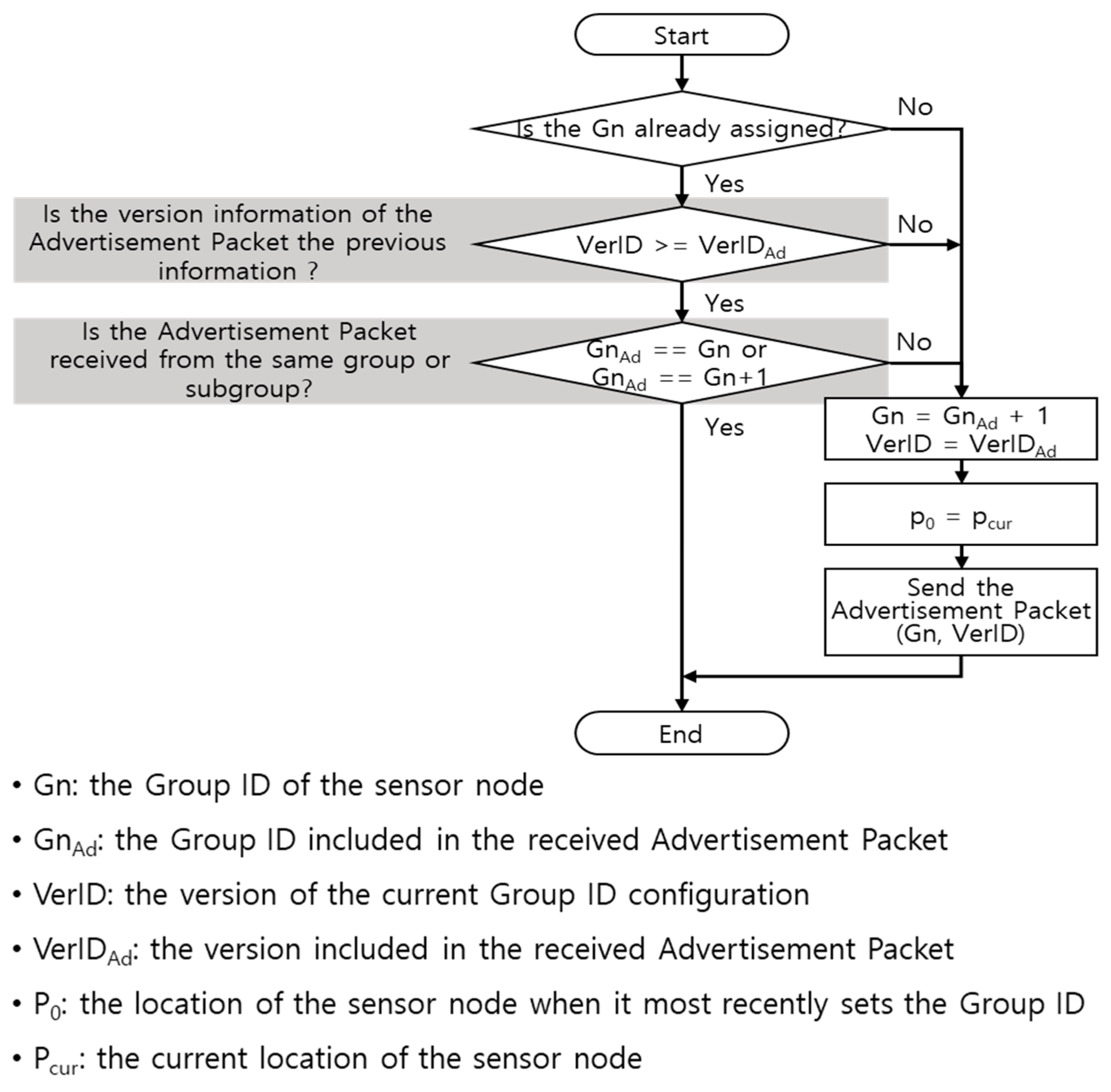
Figure 3.
Smart Sensor Node Group ID and Data Transmission Channel.

Figure 4.
Data Transmission between Smart Sensor Nodes of Different Groups.
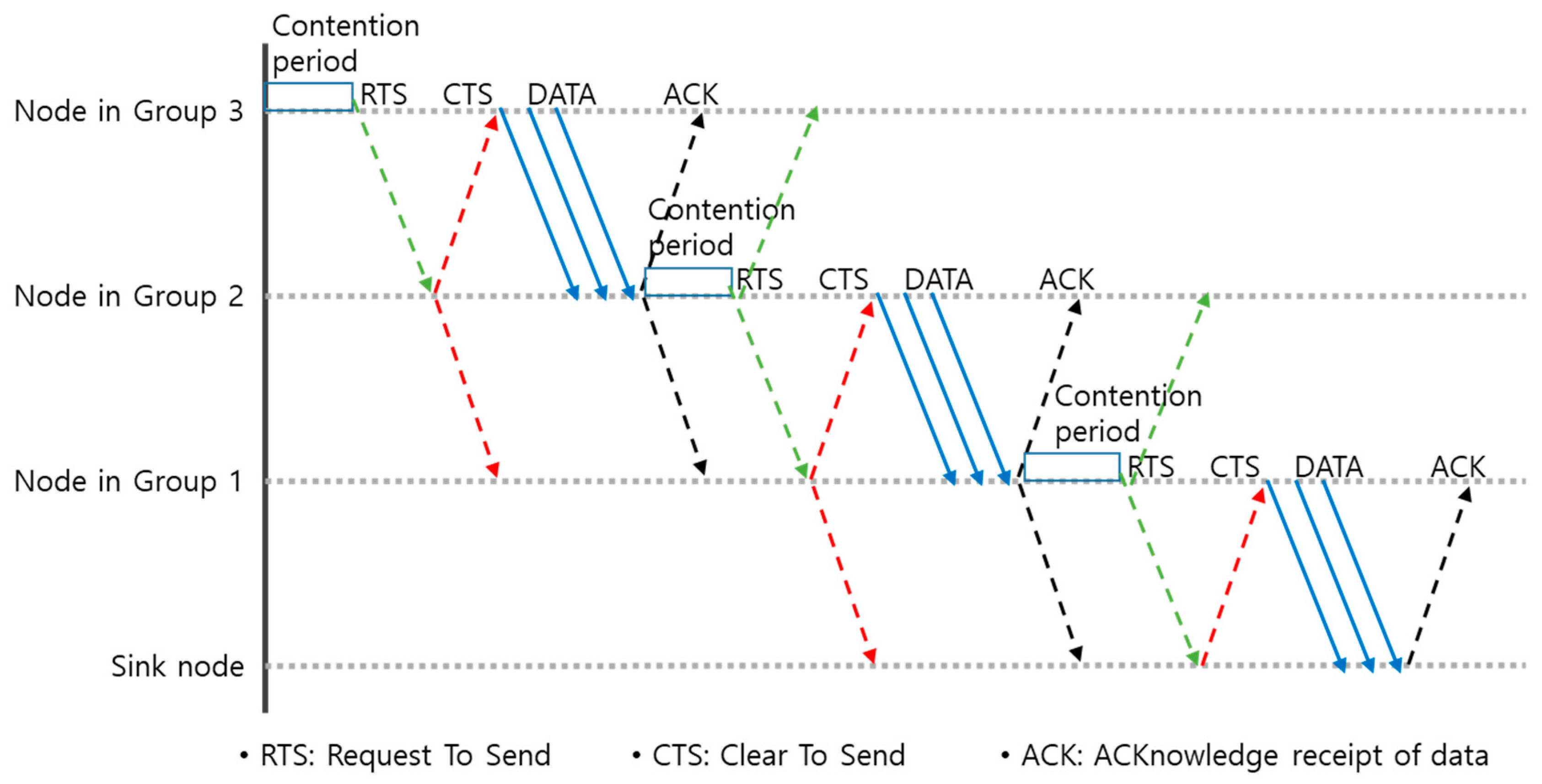
Figure 5.
How smart sensor nodes trying to reset the group ID transmit the Hello Packet, receive the Reply Packet, and set a new group ID.
Figure 5.
How smart sensor nodes trying to reset the group ID transmit the Hello Packet, receive the Reply Packet, and set a new group ID.

Figure 6.
The process where a smart sensor node receiving the Hello Packet transmits the Reply Packet.
Figure 6.
The process where a smart sensor node receiving the Hello Packet transmits the Reply Packet.
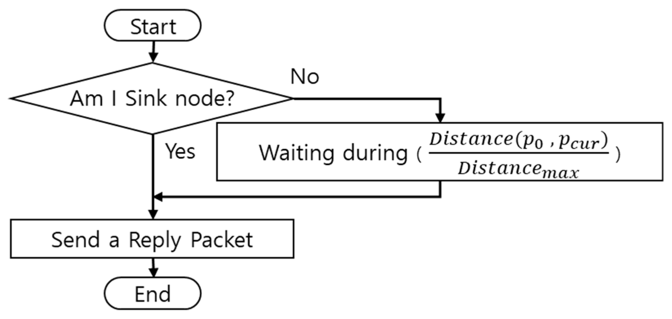
Figure 7.
Ordinary and urgent data transmission.

Figure 8.
The Network Topology for Simulation.
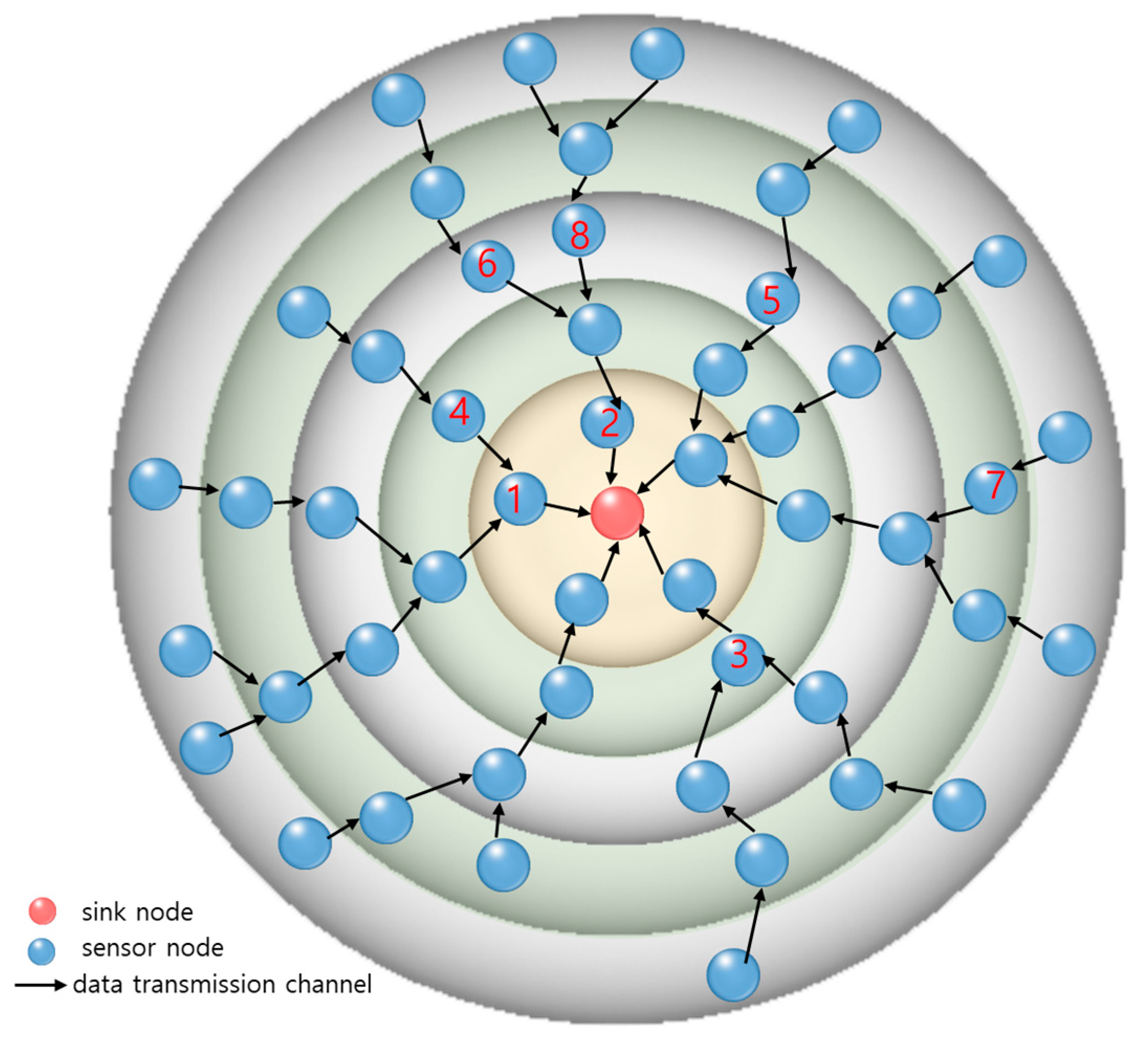
Figure 9.
Smart Sensor Node Energy Consumption Depending on the Fixed or Variable Buffer Threshold Setting
Figure 9.
Smart Sensor Node Energy Consumption Depending on the Fixed or Variable Buffer Threshold Setting
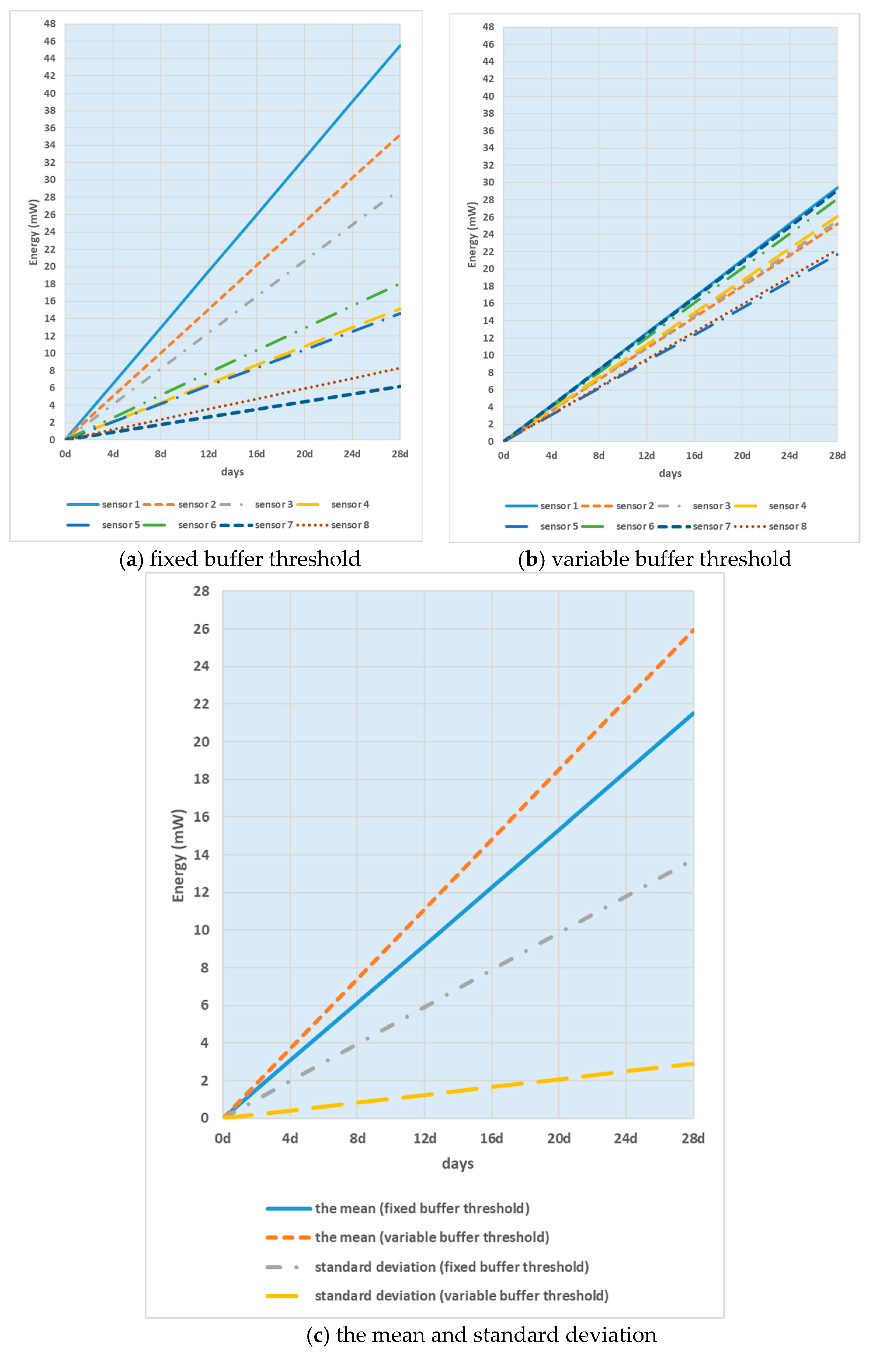
Figure 10.
Smart Sensor Node Energy Consumption Depending on Different Variable Buffer Threshold Settings.
Figure 10.
Smart Sensor Node Energy Consumption Depending on Different Variable Buffer Threshold Settings.
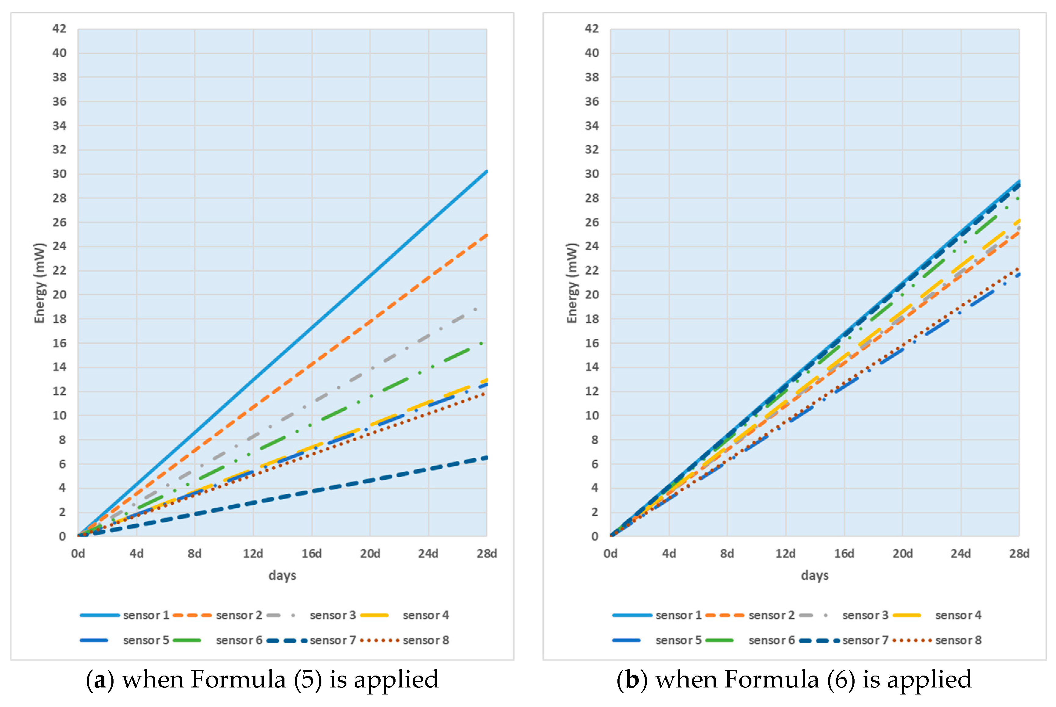

Figure 11.
The smart sensor node energy consumption of the existing MAC protocol that applies fixed buffer thresholds and the proposed method that applies variable buffer thresholds.
Figure 11.
The smart sensor node energy consumption of the existing MAC protocol that applies fixed buffer thresholds and the proposed method that applies variable buffer thresholds.

Figure 12.
Remaining energy of smart sensor nodes when the size of data was 1 B.

Figure 13.
Remaining energy of smart sensor nodes when the size of data was 10 B.

Figure 14.
Remaining energy of smart sensor nodes when the size of data was 100 B.
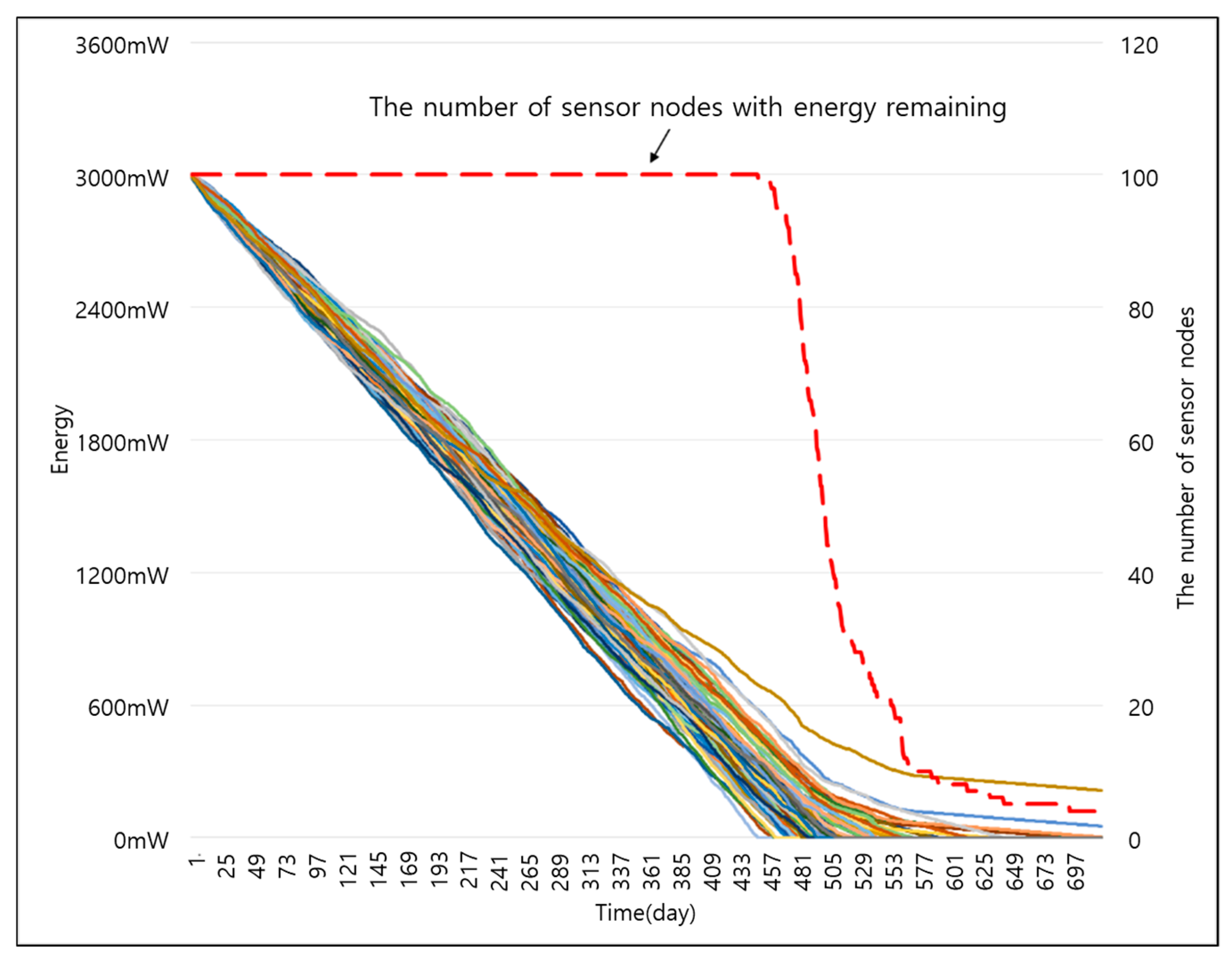
Figure 15.
Remaining energy of smart sensor nodes when the size of data was 200 B.

Figure 16.
The average duration of ordinary data transmission by smart sensor nodes of each group depending on the data size.
Figure 16.
The average duration of ordinary data transmission by smart sensor nodes of each group depending on the data size.

Figure 17.
The average duration of urgent data transmission by smart sensor nodes of each group depending on the data size.
Figure 17.
The average duration of urgent data transmission by smart sensor nodes of each group depending on the data size.

Table 1.
Simulation Environment 1.
| Components | Descriptions |
|---|---|
| System Environment (physical space) | 2 km × 2 km |
| No. of Sensor Nodes | 1 sink node, 50 sensor nodes |
| Communication Module of Sensor Nodes Applied to the Simulation | ZigBee |
| Power Consumption When a Sensor Node Transmits Data | 0.54 mW |
| Power Consumption When a Sensor Node Receives Data | 0.54 mW |
| Power Consumption When a Sensor Node Is in the Standby Mode | 0.56 mW |
| Data Generated | poisson (50) |
| Data Size | 1 byte |
| Simulation Period | 6 months |
| Parameter value α | 2 |
Table 2.
Simulation Environment 2.
| Components | Descriptions |
|---|---|
| System Environment (physical space) | 300 m × 300 m × 300 m |
| No. of Sensor Nodes | 1 Sink Node, 100 Sensor Devices |
| Communication Module of Sensor Nodes Applied to the Simulation | CC2420 Radio Transceiver Produced by Texas Instrument |
| Initial Energy of Sensor Nodes | 3000 mW |
| Power Consumption When a Sensor Node Transmits Data | 52.2 mW |
| Power Consumption When a Sensor Node Receives Data | 56.4 mW |
| Power Consumption When a Sensor Node Is in the Standby Mode | 56.4 mW |
| Max. Buffer Size of Sensor Nodes | 1024 Btyes |
| dw (the weight value for movement) | 0.5 |
| maxD (Max. Transmission Distance of Sensor Nodes) | 90 m (ZigBee Transmission Distance) |
| Data Generated | According to Poisson Distribution, Once Each Minute on Average |
| Transmission Distance Baseline for Group ID Renewal | 1 |
| Max. Movement Speed of Sensor Nodes | 5 m/min (Sink nodes and sensor nodes move randomly) |
© 2018 by the authors. Licensee MDPI, Basel, Switzerland. This article is an open access article distributed under the terms and conditions of the Creative Commons Attribution (CC BY) license (http://creativecommons.org/licenses/by/4.0/).
Share and Cite
MDPI and ACS Style
Sun, K.; Ryoo, I. A Smart Sensor Data Transmission Technique for Logistics and Intelligent Transportation Systems. Informatics 2018, 5, 15. https://doi.org/10.3390/informatics5010015
AMA Style
Sun K, Ryoo I. A Smart Sensor Data Transmission Technique for Logistics and Intelligent Transportation Systems. Informatics. 2018; 5(1):15. https://doi.org/10.3390/informatics5010015
Chicago/Turabian StyleSun, Kyunghee, and Intae Ryoo. 2018. "A Smart Sensor Data Transmission Technique for Logistics and Intelligent Transportation Systems" Informatics 5, no. 1: 15. https://doi.org/10.3390/informatics5010015
Note that from the first issue of 2016, this journal uses article numbers instead of page numbers. See further details here.