Article

Towards Clustering of Mobile and Smartwatch Accelerometer Data for Physical Activity Recognition

1
Department of Computer Science, Liverpool John Moores University, Byrom Street, Liverpool L3 3AF, UK
2
Department of Computer Science, University of Rochester, 3700 Wegmans Hall, P.O. Box 14620, Rochester, NY, USA
*
Author to whom correspondence should be addressed.
Informatics 2018, 5(2), 29; https://doi.org/10.3390/informatics5020029
Submission received: 1 March 2018 / Revised: 7 June 2018 / Accepted: 8 June 2018 / Published: 12 June 2018
(This article belongs to the Special Issue Sensor-Based Activity Recognition and Interaction)

Abstract

:
Mobile and wearable devices now have a greater capability of sensing human activity ubiquitously and unobtrusively through advancements in miniaturization and sensing abilities. However, outstanding issues remain around the energy restrictions of these devices when processing large sets of data. This paper presents our approach that uses feature selection to refine the clustering of accelerometer data to detect physical activity. This also has a positive effect on the computational burden that is associated with processing large sets of data, as energy efficiency and resource use is decreased because less data is processed by the clustering algorithms. Raw accelerometer data, obtained from smartphones and smartwatches, have been preprocessed to extract both time and frequency domain features. Principle component analysis feature selection (PCAFS) and correlation feature selection (CFS) have been used to remove redundant features. The reduced feature sets have then been evaluated against three widely used clustering algorithms, including hierarchical clustering analysis (HCA), k-means, and density-based spatial clustering of applications with noise (DBSCAN). Using the reduced feature sets resulted in improved separability, reduced uncertainty, and improved efficiency compared with the baseline, which utilized all features. Overall, the CFS approach in conjunction with HCA produced higher Dunn Index results of 9.7001 for the phone and 5.1438 for the watch features, which is an improvement over the baseline. The results of this comparative study of feature selection and clustering, with the specific algorithms used, has not been performed previously and provides an optimistic and usable approach to recognize activities using either a smartphone or smartwatch.

1. Introduction

The idea of wearing on-board computing systems has been around since the 1980s [1]. However, recent advances in wireless communication technologies, embedded systems, and the lower costs of components (e.g., batteries, processors, and sensors) have enabled these devices to become more miniaturized and mainstream [2]. The advent of smaller and more powerful devices has enabled technology to take a more central role in everyday life and has enabled personal experiences, such as capturing photographs, videos, or tracking fitness, to become common practice. Every moment of daily life can be shared digitally and can be enriched in ways that we could not have imagined years ago [3]. Part of such developments has been the inception of wearable devices (e.g., smartwatches, health and fitness trackers, etc.) that have exploded onto the consumer market. By 2019, Cisco predicts that there will be 578 million wearable devices globally, which is a fivefold increase from 109 million in 2014 [4]. These devices now house a multitude of sensors that are capable of capturing a large amount and range of personal information. Consequently, with all of this data readily available, end users have become more interested in quantifying their activities through their collected personal data. It has been this interest and explosion of consumer wearable products that has paved the way for the areas of lifelogging and the Quantified Self [5] to thrive, as users can actively track themselves over a sustained period of time [6]. These devices flourish in the field of activity recognition, where they can function continuously without human intervention or maintenance [1]. This area has been gaining great momentum due to the tremendous benefits that are associated with long-term monitoring and has garnered interest from researchers and clinicians [7,8,9]. For instance, a system that monitors and gathers data, over a sustained period of time, could significantly improve the prevention, diagnosis, and treatment of several noncommunicable diseases, including obesity and depression [8,10]. As the system gathers more information about the user, it can “learn” about his or her lifestyle. These patterns of behaviour can then be analyzed (see previous work [11]) to recommend healthy lifestyle changes and users can also use this information to reflect on their levels of activity to improve their quality of life [12].
One continuous trend in electronics seems to be hardware miniaturization [13]. For example, Kryder’s law explains that physical storage size is reducing continuously and increasing in capacity in a logarithmic scale [14]. Similar advances are also applicable in the miniaturization of sensors. These ongoing trends suggests that wearables and other ubiquitous devices either already have or soon will have enough capability to host their own data for the long term [15]. However, such developments in capturing and storing data have outpaced current knowledge on processing this information. Whilst we have access to a number of consumer products that are capable of recording data, a major challenge in this area is processing this data to extract relevant information [7]. As devices have become smaller and more powerful, data analysis tools have not been as fortunate and often appear rudimentary when compared to the data collection devices [16]. Mobile devices and smartwatches are equipped with several sensors, including accelerometers, which can quantify physical activity. However, such sensors produce large sets of raw data. It is unfeasible to feed raw data or a large number of features into algorithms. Furthermore, detecting physical activity is often treated as a classification task, which is dependent on labelling data in a valid fashion, i.e., accurately representing a distinction between multiple activities [17,18,19]. This limits real-world applicability as labels are derived offline, after the event. Furthermore, self-reports tend to overestimate the time spent in unstructured daily physical activities or momentary sporting physical activities, which are the two main aspects of human physical activities [20]. However, clustering can be used to overcome this challenge as it significantly reduces the search space and does not require the data to be labelled via user input.
In addressing this issue, this paper presents our approach that utilizes two feature selection approaches, principle component analysis feature selection (PCAFS) and correlation feature selection (CFS), to improve the clustering of accelerometer data for the purposes of activity recognition. The motivation behind utilizing feature selection is due to the limitations of mobile and wearable devices. Feeding raw data or a large number of features into clustering algorithms is not efficient. By removing redundant features, we are limiting the search space by selecting a subset of the most important features that can be used to describe the majority of the data. Raw accelerometer data from mobile devices and smartwatches have been obtained from the publicly available Heterogeneity Human Activity Recognition Dataset (HHAR) [21]. The main contributions of the paper are to utilize feature selection to reduce the baseline feature set by removing redundant features and to evaluate our feature selection approaches, in terms of the quality of the clustering, against the baseline using hierarchical clustering analysis (HCA), k-means, and density-based spatial clustering of applications with noise (DBSCAN). This comparative study of feature selection and clustering has not been performed previously in this manner. This will enable us to determine how well the selected features perform within the clustering algorithms in separating instances of human activity and the performance of each clustering algorithm. The remainder of this paper is constructed as follows. Section 2 presents an overview of related work, whilst Section 3 describes the materials and methods that have been used to preprocess the data, extract and select features, as well as the clustering processes. Section 4 presents the results of the data evaluation, while Section 5 discusses the results. The paper is then concluded in Section 6 and future directions of the research are presented.

2. Related Work

As wearable devices become more widespread, it has become easier to record our activities and experiences. Recent technological developments have made the use of such devices, such as the accelerometers and heart-rate monitors, popular within the consumer market and within research domains, such as lifelogging, epidemiology, and other health-related areas [16,22,23]. There have been many approaches within the field of wearable sensing that aim to detect human activity [7,18,24,25].
As noted by Morales and Akopian [26], in most instances, accelerometer signals and machine learning are used for activity detection. For instance, Qiu et al. [18] used accelerometer data from a SenseCam and machine learning tools to automatically identify user activity. In their approach, a support vector machine (SVM) was trained to automatically classify accelerometer features into user activities (sitting or standing, driving, walking, or lying down) [18]. Meanwhile, Uddin et al.’s [24] wearable sensing framework utilized a nine-axis wristband to continuously monitor users’ daily activities. The data was then preprocessed and segmented before being passed to the activity recognition algorithm. In other works, Saeedi et al. [25] developed an automatic on-body sensor platform, consisting of accelerometers and gyroscope sensors, to monitor physical activity. The k-nearest neighbors (kNN) classifier was then used to categorize the activities and achieved an average recall of 98.41% and precision of 98.42%.
In other works, Machado et al. [7] used unsupervised learning to detect human activity from two triaxle accelerometers placed on the waist and wrist. The results indicate that the k-means algorithm produced highly accurate results and was able to recognize various activities, such as standing, sitting, and walking. However, this is in contrast to our approach, which uses different methods of feature extraction and selection to reduce the number of features that are being used. As the accumulation of data increases, the need to provide more accurate ways of analyzing this information is evident. As these datasets grow in size, performing complex clustering on very large datasets becomes less practical, as accuracy is compromised. Taking a different approach, Fortino et al. [27] explored community-scale cloud-based activity recognition with their BodyCloud system. This approach is a cloud-based multitier application-level architecture that integrates the SPINE BAN middleware with a cloud computing platform. The idea is to support the rapid and effective development of community body area network applications through programming abstractions, such as group, modality, workflow, and view. However, there are some issues with relying on the cloud to process data, including bandwidth and latency (i.e., how long it takes for the system to react to an activity transition) [26]. Nevertheless, as noted by Lara and Labrador [28], there are still many challenges in this area, including the selection of attributes and sensors, obtrusive sensing, data collection protocols, recognition performance, energy consumption, processing, and flexibility.

3. Materials and Methods

Our approach utilized a data processing pipeline to process raw accelerometer data, which included extracting and selecting features before clustering can occur (see Figure 1).
This study utilized data that had been obtained from accelerometer sensors found within smartphones and smartwatches [21]. This type of sensor is widely supported in existing mobile and wearable devices on the market and is extensively used in the area of activity recognition [2,16,29]. The remainder of this section expands on the steps that have been illustrated in Figure 1.

3.1. Raw Data

Raw data had been obtained from two publicly available datasets found within the Heterogeneity Human Activity Recognition Dataset (HHAR) [21]. The smartphone dataset contained 11,279,275 instances of raw time-series tri-axil accelerometer data that had been recorded from eight smartphones (2 × Samsung Galaxy S3 minis, 2 × Samsung Galaxy S3s, 2 × LG Nexus 4s, and 2 × Samsung Galaxy S+). From here on out, this dataset will be referred to as the Phone dataset. The smartwatch dataset contained 3,020,605 instances of raw time-series tri-axil accelerometer data that had been recorded from four smartwatches (2 × LG watches and 2 × Samsung Galaxy Gears). From here on out, this dataset will be referred to as the Watch dataset. Each dataset contained recordings from nine users. Each volunteer undertook a series of six activities, including sitting, standing, biking, walking, walking up stairs, and walking down stairs, and adhered to the data collection protocol, which included performing each activity for five minutes. The total number of data items was 14,299,880 instances of raw activity data. One aspect of these datasets is that each device yields different sampling frequencies, which is problematic when preprocessing the data, as certain methods are frequency dependent. In this work, each device was preprocessed separately before features were then extracted individually for each device. Table 1 depicts a summary of the devices and their associated sampling frequencies (Hz).
To test the validity of our approach, the baseline method was compared against two feature selection methods. The baseline approach utilized all the generated features, whilst the feature selection methods included: (1) principle component analysis feature selection (PCAFS); and (2) correlation feature selection (CFS). These approaches were used to reduce the baseline feature set by removing redundant features. Applying these feature selection approaches allowed us to select a subset of the most important features and to determine if the baseline results could be improved upon and to determine the best way to reduce the features.

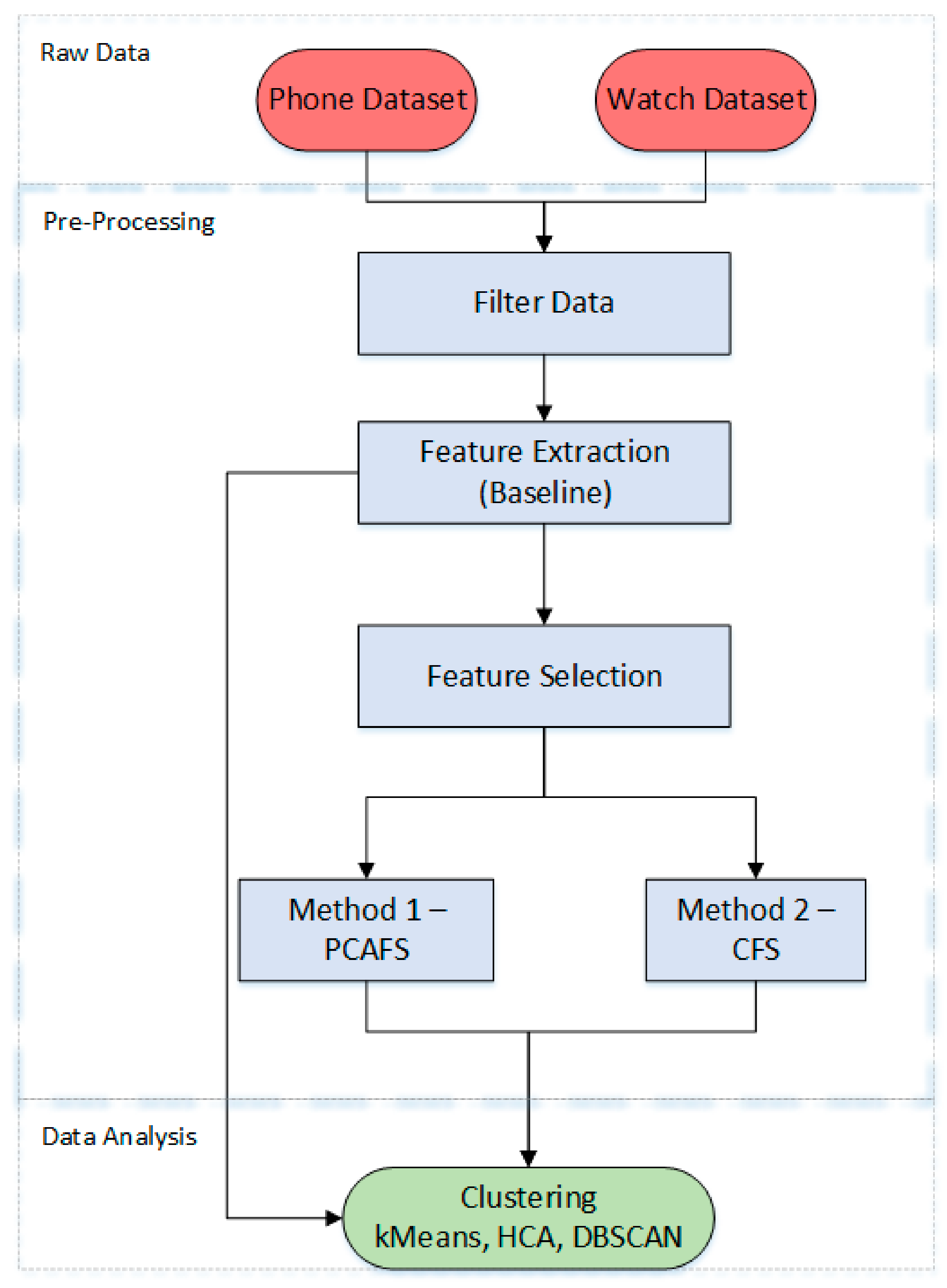
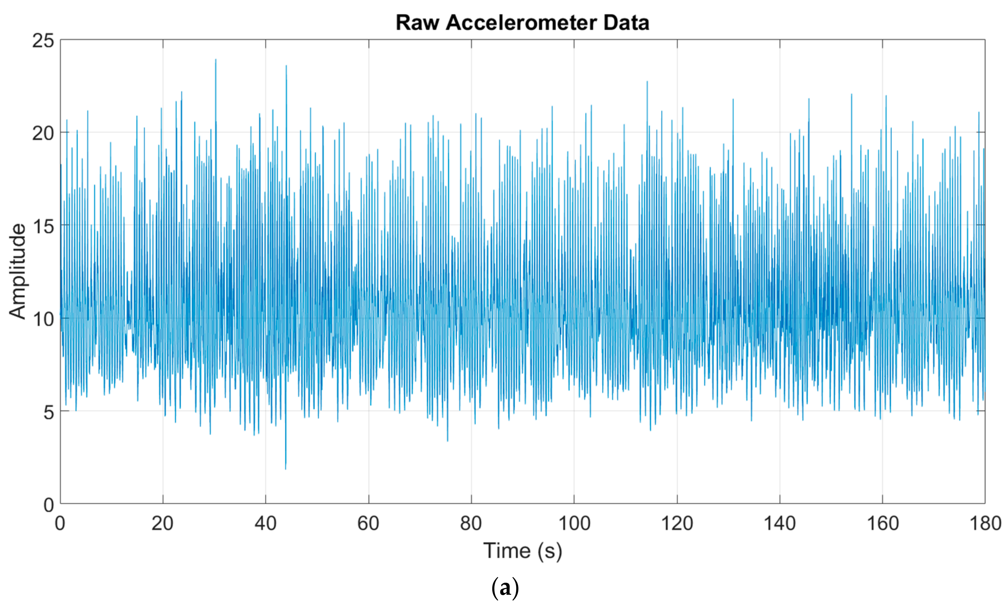
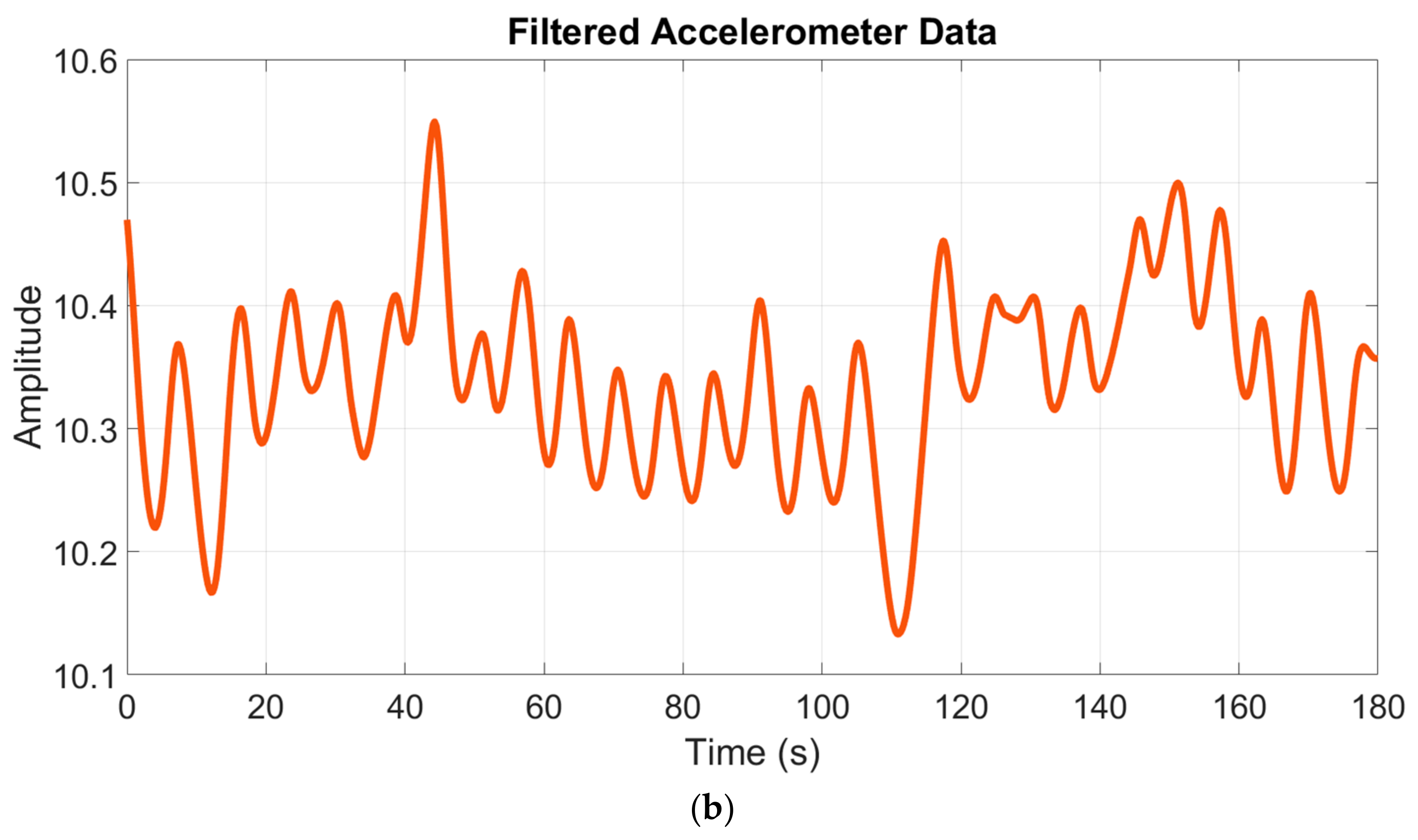
3.2. Preprocessing and Feature Extraction

The first step in the pipeline was to preprocess the accelerometer data by first combining the raw accelerometer axes (x, y, and z) into a single vector using Equation (1):
a =   x 2 +   y 2 + z 2
Combining the axis allowed for the overall vector magnitude to be obtained, which accounted for overall movement. This is a standard method of processing accelerometer data [21,30,31]. The raw data were then filtered using a second-order forward-backward digital low-pass Butterworth filter, with a cut-off frequency of 3 Hz (see Figure 2). As demonstrated in previous works [32,33,34], this cut-off frequency is appropriate to filter the data without losing any information.
Using Equation 2, the data were then normalized (n). The filtered data (x) were divided by their maximum absolute value. A sliding window of 2 s, with a 50% overlap, was also applied to the data. In previous works [21,35,36,37,38,39,40], this size produced the best results, whilst ensuring that different activities can still be recognized.
n =   x max | x |
Standard activity related features, which had been compiled from analyzing the literature [35,36,37,38,39,40,41,42,43,44,45], were then extracted from the filtered data over both the time and frequency domains. This was because within the time domain, simple mathematical and statistical metrics can be used to extract basic signal information from raw sensor data over a period of time [46]. In contrast, frequency domain analysis depicts how the signal’s energy is distributed over a range of frequencies [47]. Frequency domain techniques have been extensively used to capture the repetitive nature of a sensor signal. This repetition often correlates to the periodic nature of a specific activity, such as walking or running [46]. The advantage of frequency-related parameters is that they are less susceptible to signal quality variations [48].
The following features were extracted from the time domain—mean, median, standard deviation (STD), root mean square (RMS), and variance. In order to undertake frequency domain analysis, a mathematical operator called a transform was used to convert the signal from the time domain into the frequency domain. Fast Fourier transform (FFT) and power spectral density (PSD) were both used to transform the signal. Prior to calculating the FFT and PSD, the direct current (DC) component first had to be removed, as was the case in several studies [36,44,45]. The DC component is the mean acceleration of the signal [45] and is removed so that the signal is not distorted, as this value is often much larger than the remaining coefficients [46]. The following features were extracted from the frequency domain—energy, entropy, and mean frequency. Energy has been used to characterize the frequency components of each activity, whilst entropy illustrates the consistency in an activity, which is useful to differentiate between signals that have similar energy values but correspond to different activity patterns [37]. These standard statistical features were chosen because they represent a range of information about the signal. Table 2 provides a summary of the features that have been extracted.
This method provided an approach that enabled raw data to be condensed into a smaller amount of more useful information. These features comprised the complete baseline feature set. Within the Phone dataset 770,184 feature records were generated, whilst the Watch dataset contained 135,792 records, thus totaling 905,976 records.

3.3. Feature Selection

Once the features had been generated, dimensionality reduction was performed in order to find a subset of the most important features. This step was necessary to ascertain whether the results could be improved and to reduce the searching space, as some of the generated features might be unnecessary [49]. However, choosing the optimum number of features is usually challenging [50]. However, a scree plot can be used to overcome this issue. This graph plots the generated eigenvalues and arranges them in descending order. The point at which the curve of decreasing eigenvalues decelerates to a flat slope (also known as the “elbow”) is the cut-off point and determines the number of features to use [51,52]. Each dataset was analyzed separately. Figure 3a illustrates the generated scree plot of the Phone dataset, whilst Figure 3b illustrates the generated scree plot of the Watch dataset. As can be seen in Figure 3, the optimal number of features to use for both the Phone and Watch datasets was two. This indicates that out of the eight original features from Table 2, two had the best discriminative capabilities to represent the datasets.

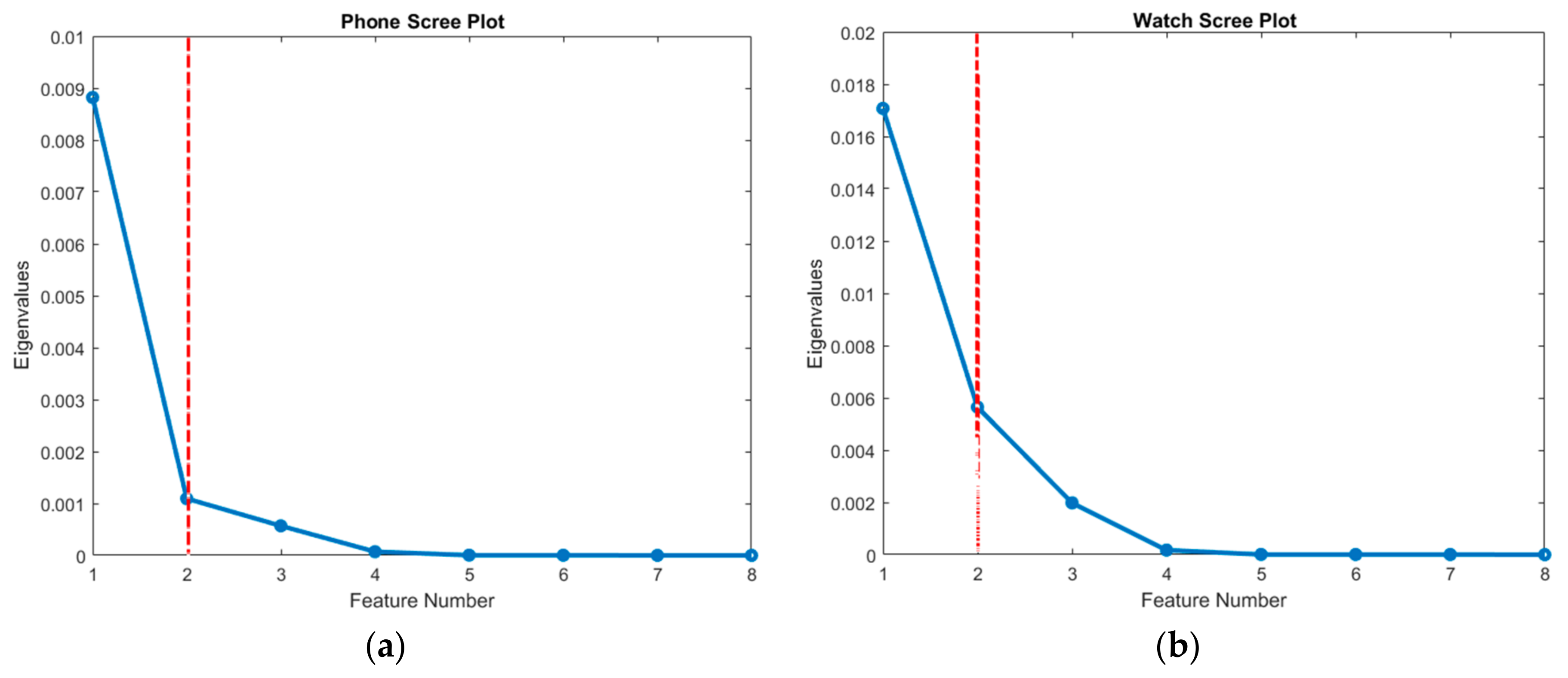
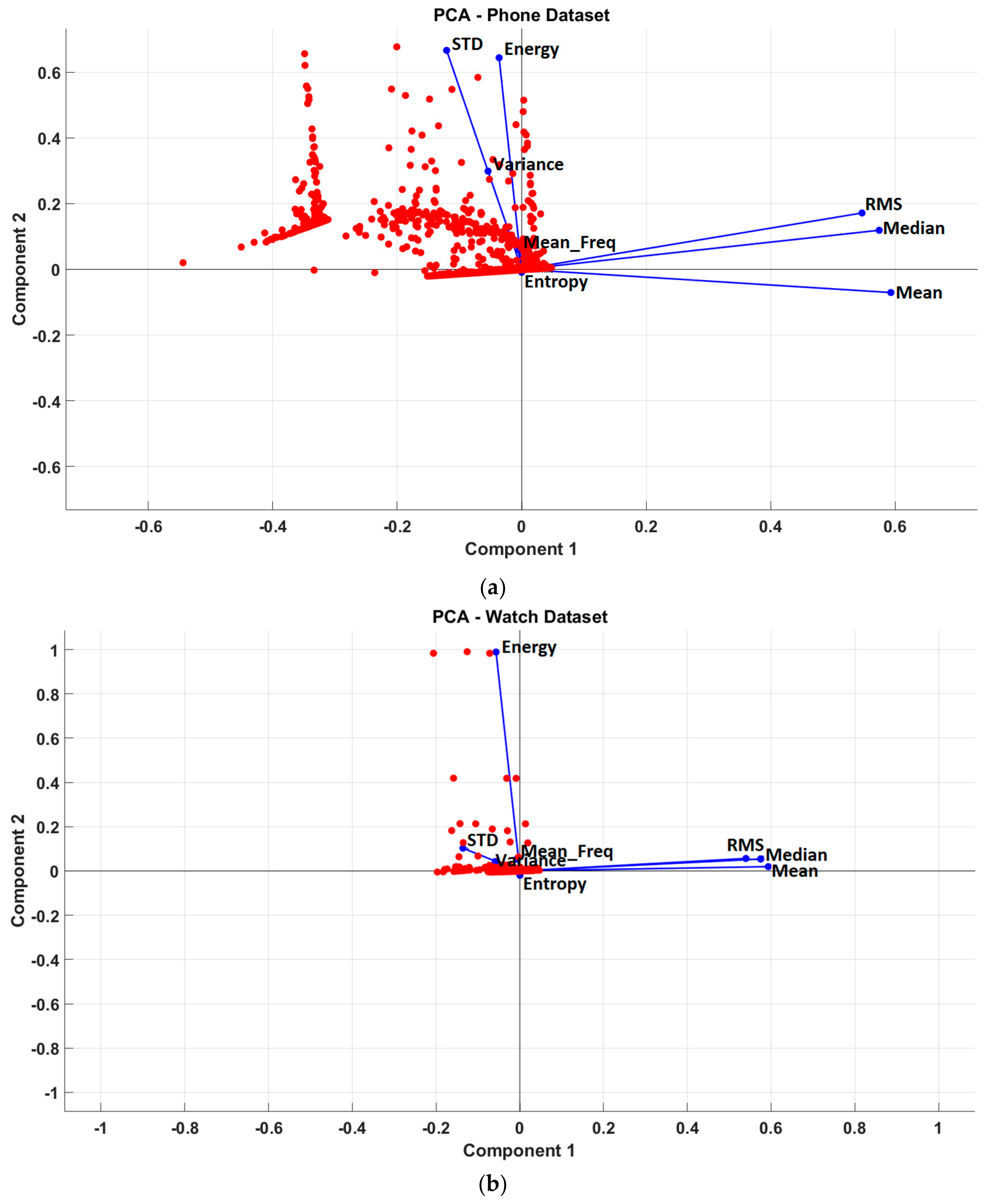
3.3.1. Method 1—Principle Component Analysis Feature Selection (PCAFS)

Our first feature selection method used principle component analysis (PCA) to identify the two features that had the best discriminative capabilities and thus contained the most information. During PCA, three components were calculated—eigenvalues, eigenvectors, and scores. Eigenvalues measure the amount of variation explained by each principle component, with the first coefficient being the largest. Eigenvectors are a linear combination of the original variables and have a corresponding eigenvalue. Scores are used in the bi-plot to represent the data by illustrating how close the features are to the first and second principle components.
Figure 4a illustrates the PCA graph that was generated for the Phone dataset, whilst Figure 4b illustrates the PCA graph for the Watch dataset. Each feature in the bi-plot of Figure 4 is represented as an eigenvector and the direction and length of the vector (blue line) indicates how each variable contributes to the principal components in the plot. In selecting the best features, we needed to look for the features on the bi-plot that had large vectors and positive coefficients for both components.
From the scree plots shown in Figure 3, we knew that the optimal number of features to use for both datasets was two. Figure 4a illustrates that the best two features of the Phone dataset were Root Mean Square (RMS) and Median, whilst Figure 4b illustrates that the best two features of the Watch dataset were Mean and Median. These features were chosen because they displayed the largest positive vectors for both components. This was important because the first principle component (component 1) contained most of the variance and the largest eigenvector contained all positive instances. These were used to evaluate the effectiveness of the PCAF method within the clustering algorithms.

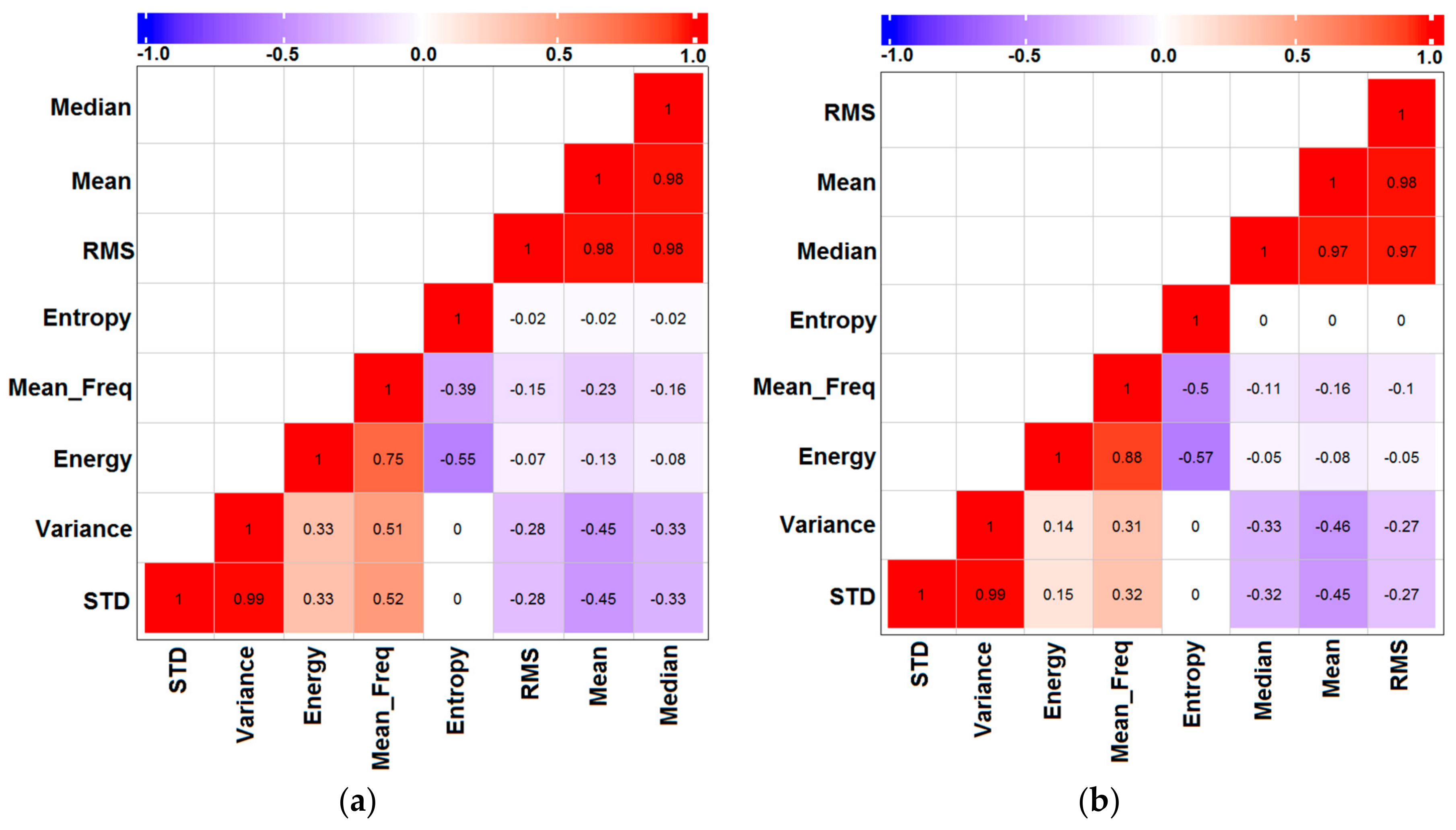
3.3.2. Method 2—Correlation Feature Selection (CFS)

Our second method used Pearson correlation (see Equation (3)) to identify the correlations between the features. In this equation, the linear correlation r is computed for each pair of features (x, y). Here, x k ¯ and y k ¯ denotes the mean of x and y, with the resulting correlation coefficient being between −1 and 1 [53].
r =   k ( x k     x k ¯ ) ( y k   y k ¯ ) k ( x k   x k ¯ ) 2   k ( y k   y k ¯ ) 2
If x and y are linearly correlated, then r will be within the scale of 1 to −1. However, if the features are completely independent (i.e., uncorrelated) than r will be 0 [53,54]. In this case, features that are strongly correlated between each other may be removed. Therefore, if the correlation between sets of features is low, then they are regarded as suitable features to use [53]. Figure 5 illustrates heat maps that depict the relationship between the features of both datasets.
The coefficients denoted in Figure 5 illustrate that a number of separate features share almost total positive correlation. From Figure 5a,b, we can see that (variance, standard deviation (STD)), (mean, root mean square (RMS)) (median, root mean square (RMS)), and (median, mean) had an almost total positive correlation of 0.97–0.99 across both datasets. Therefore, when clustering the data, only the features with a correlation of 0 were selected, which included (entropy, standard deviation (STD)) and (entropy, variance) for the Phone dataset. For the Watch dataset, the features included (entropy, standard deviation (STD)), (entropy, variance), (median, entropy), (mean, entropy), and (root mean square (RMS), entropy). As the optimal number of features to select was two, each pair of features was evaluated within the clustering algorithms.
In summary, this section has illustrated two approaches that can be used to select a subset of features in order to reduce the dimensionality of the dataset. Table 3 provides a summary of the combination of features that were selected from each method.
These features were used within the evaluation. However, as the CFS approach yielded multiple combinations of features, each set was analyzed separately. In this instance, for the Phone dataset, (Entropy, STD) was labelled as Phone1, whilst (Entropy, Variance) was labelled as Phone2. Similarly, for the Watch dataset, (Entropy, STD) was labelled as Watch1, (Entropy, Variance) as Watch2, and so on.

3.4. Clustering Algorithms

Our approach utilized a comparison between HCA (hierarchical clustering), k-means (partitioning), and DBSCAN (density-based) clustering algorithms. Due to its ease of implementation, simplicity, efficiency, and empirical success, the most popular algorithm for clustering is k-means [55,56,57,58]. It is a simple iterative method that is used to partition n observations into a user-specified number of clusters, k [57,59]. The data objects are grouped together into “compact” clusters with the assumption that all objects, within one group, are either mutually similar to each other or they are similar with respect to a common representative or centroid [60]. The centroid is the mean position of the clusters and this is then initialized. Each object is then assigned to its nearest centroid (cluster) and the mean of the new centroids (clusters) is then calculated. This process is repeated until the centroids (clusters) do not change.
Alternatively, in hierarchical clustering analysis (HCA), each object initially represents a cluster of its own, and they are sequentially merged until the desired cluster structure is obtained [61]. In order to perform this type of clustering, the similarity between pairs of objects first needs to be calculated. Similar objects are then grouped together to form large cluster trees. Branches at the bottom of the tree are trimmed, objects at the bottom are assigned to other clusters, and dendrograms are then created to represent these groups of data. Density-based spatial clustering of applications with noise (DBSCAN) is another common algorithm that searches the region of each object to ascertain if it contains more than the minimum number of objects [62]. Clusters are then created from all data objects in that region [63]. DBSCAN can be advantageous over k-means because DBSCAN is less sensitive to noise and allows clusters of arbitrary shape whilst providing deterministic results [59]. However, a drawback of DBSCAN is that when clusters of different densities exist, only particular kinds of noise points are captured. Furthermore, it does not perform well when clusters are close and border each other [64].

4. Results

This section presents the results that have been obtained from our approach to clustering the data using (1) k-means, (2) hierarchical clustering analysis (HCA), and (3) density-based spatial clustering of applications with noise (DBSCAN). The evaluation first uses the baseline Phone and Watch datasets, which utilizes all of generated features, to assess the algorithms performance. The experiments have then been repeated with the PCAFS datasets and the CFS datasets, which utilize a subset of the baseline features to establish if the results can be improved. We have used the internal and external measures Dunn Index (DI), distance ratio (DR), and entropy (EN) as validation mechanisms to assess the quality of the clustering algorithms with the various feature selection methods [26,65]. A higher DI implies that clusters are compact and well-separated from other clusters. Distance ratio has been calculated by dividing the average distance within clusters by the average distance between clusters. This measurement is a ratio of the mean sum of squares within clusters to the mean sum of squares between clusters. Entropy is a measure of uncertainty and is the average (expected) amount of the information from an event. In assessing these approaches, high DI and DR and low EN are preferable in assessing the algorithm’s ability to separate the data. In each experiment, the k-means algorithm uses the silhouette averages from Table 4 to denote k. The evaluation platform that has been used was a Windows® 10 64-bit Intel® Core ™ i7-3770 central processing unit (CPU) at 3.40 GHz with 32 GB of random-access memory (RAM). These experiments have been conducted using RStudio v0.99.903.

4.1. Determining k for k-Means Clustering

A requirement of the k-means algorithm is that the user needs to define the number of clusters (k) beforehand. This is the most critical user-specified parameter, with no perfect mathematical criteria [55]. Therefore, defining k can be challenging and may be seen as a drawback [59], as the best number of clusters can be difficult to distinguish. However, silhouette averages are often used as a useful measurement for selecting the “appropriate” number of clusters, as it gives an idea of how well separated the clusters are [58,66]. The silhouette value S(i) quantifies the similarity of an object i to the others in its own cluster, compared to the objects in other clusters [58,66]. These values range from +1, indicating points that are very distant from neighboring clusters, through to 0, indicating points that are not distinctly in one cluster or another, to −1, indicating points that are probably assigned to the wrong cluster. The silhouette average (SA) is then calculated and is used as a measurement of the quality of the resulting clusters [58]. The value of k that has the largest SA indicates the most appropriate value to use. Using the baseline, PCAFS, and CFS datasets, the value of k has been increased, from two to six, and evaluated using the silhouette averages (see Table 4).
As previously stated, the most appropriate number of clusters (k) to use for each dataset are determined by the largest SA. As it can be seen in Table 4, for the baseline Phone dataset, it is three, whilst for the Watch dataset, it is four. In relation to the PCAFS method, it is two for the Phone and three for the Watch, whilst for the CFS Phone1, Phone2, Watch1, Watch2, and Watch5, it is also two, whilst for Watch3 and Watch4, it is three. These values of k will be used within the results to implement the k-means clustering algorithm. It should be noted that hierarchical clustering analysis (HCA) and density-based spatial clustering of applications with noise (DBSCAN) do not require k to be specified.

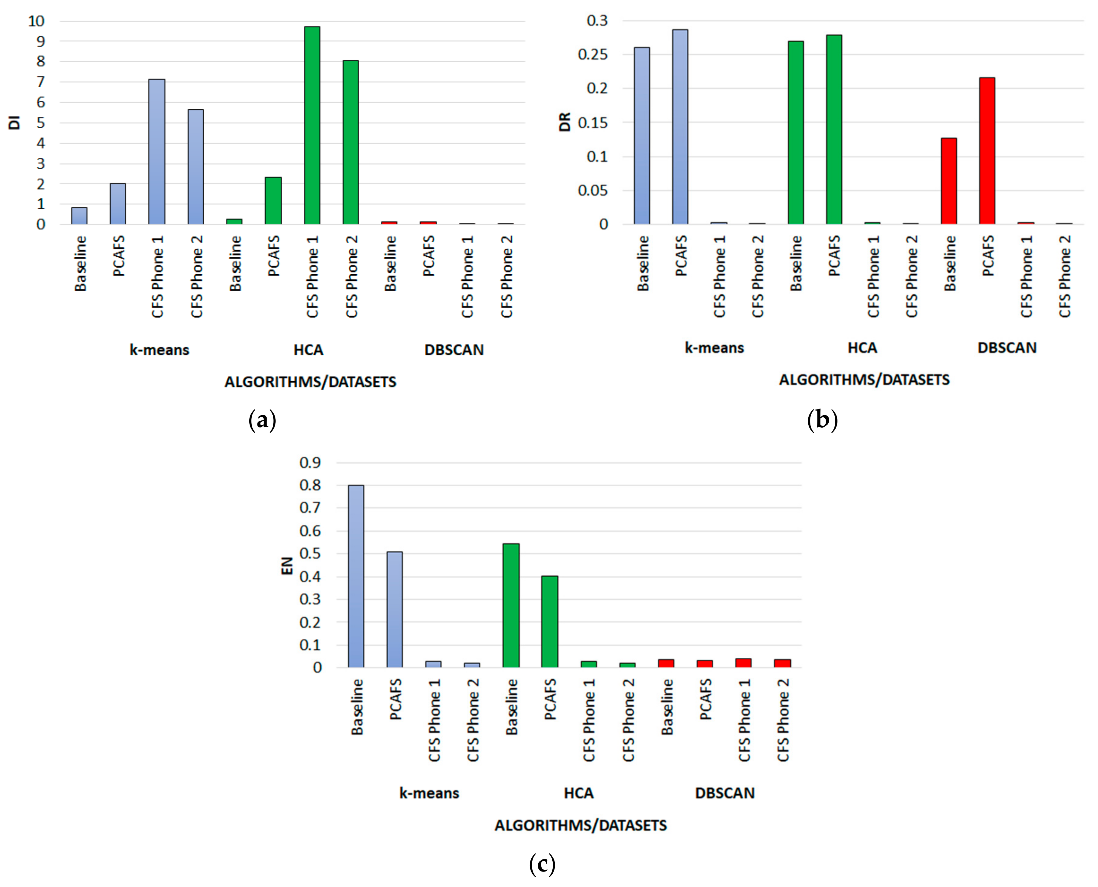
4.2. Results of the Phone Datasets

Figure 6 presents the results of the Phone datasets using the validation measures above and the baseline feature set, as well as the reduced PCA and CFS feature sets.
The results from Figure 6 illustrate that, using the baseline feature set, k-means produced the highest DI (0.8460), whilst HCA produced a slightly better DR (0.2705), and DBSCAN produced the lowest entropy (0.0377). However, when the feature set is reduced, these results improve upon the baseline. Looking to the PCAFS approach, k-means produced the highest DR (0.2866), whilst HCA performed better in terms of higher DI (2.3123), and DBSCAN again produced the lowest EN (0.0332). Using the CFS approach, HCA produced the best results using Phone1, which obtained a higher DI (9.7001) and DR (0.0028). Overall, the CFS feature selection approach and the HCA algorithm produced the best DI (9.7001) and EN (0.0187). This implies that these clusters are quite compact, well separated, and that uncertainty is reduced. DBSCAN appears to perform the worst.

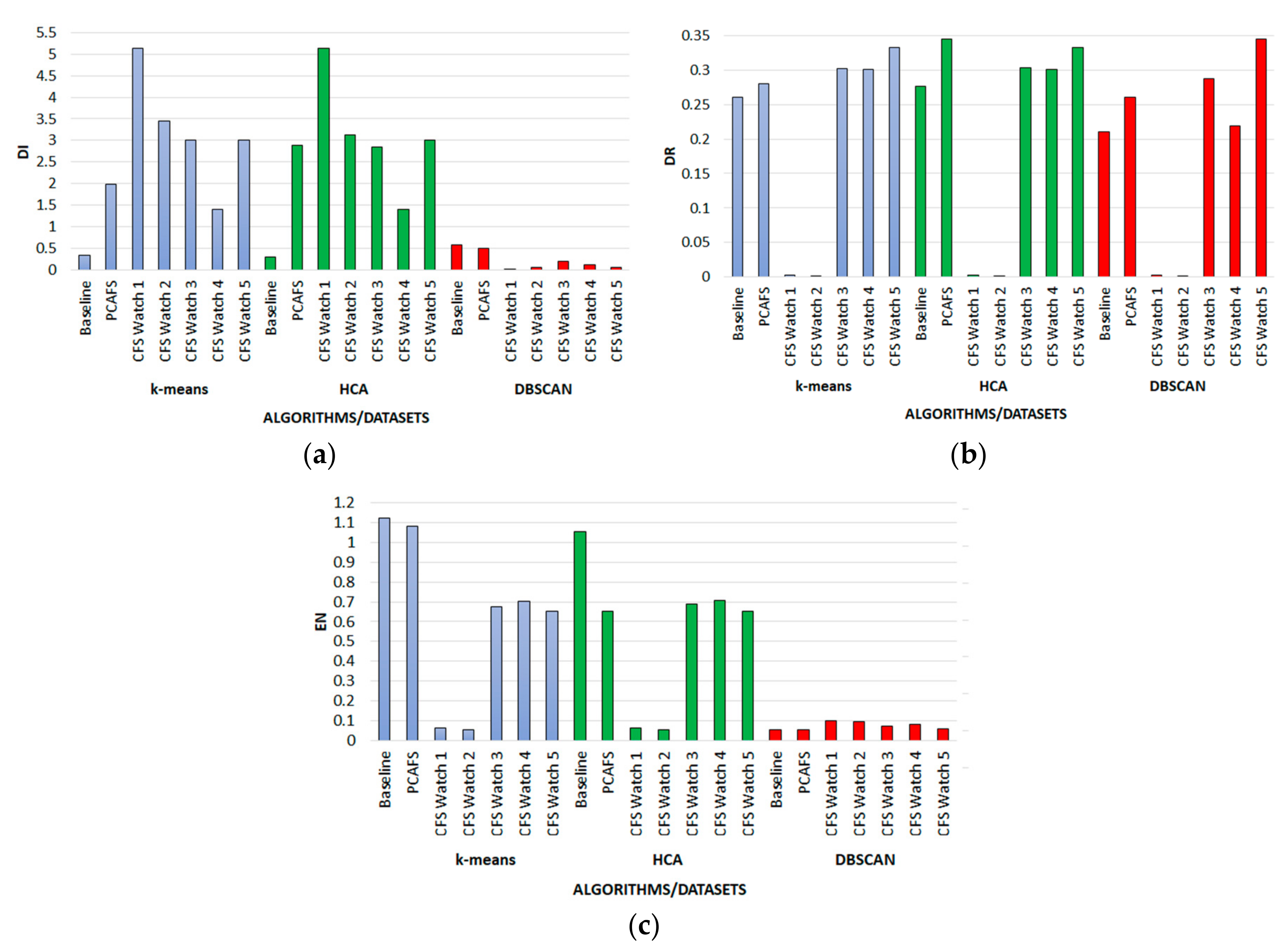
4.3. Results of the Watch Datasets

Figure 7 presents the results of the Watch datasets using the validation measures above and the baseline feature set, as well as the reduced PCA and CFS feature sets.
The results from Figure 7 illustrate that, using the baseline feature set, DBSCAN performed better in terms of higher DI (0.5804) and lower EN (0.0556), whilst HCA had a higher DR (0.2767). However, reducing the feature set has again improved these results. Using the PCAFS approach, HCA produced the highest DR (0.3449) and DI (2.8879), whilst DBSCAN produced the lowest EN (0.0524). Using the CFS approach k-means and HCA seemed to perform the best using Watch1, which obtained equally high DIs (5.1438). Overall, the CFS feature selection approach produced the best results in terms of high DI (5.1438) using both k-means and HCA, a high DR using DBSCAN (0.3452), and low EN using k-means (0.0515). In summary, the feature selection algorithms have significantly improved upon the baseline results. In particular, the CFS approach has performed the best across both datasets using k-means and HCA. For instance, the results illustrate that, using the Phone dataset, CFS and HCA produced the highest DI (9.7001) and lowest EN (0.0187). Meanwhile, using the Watch dataset, CFS and k-means produced the highest DI of 5.1438 and lowest EN of 0.0515. As a higher DI implies that clusters are compact and well-separated from other clusters, it would appear that the Phone dataset outperformed the Watch dataset. DBSCAN appears to perform the worst using both sets of data.
Since the CFS approach, in conjunction with HCA, produced the best results using Phone1 and Watch1, simplified visualizations have been produced to reflect the classes with which the clusters are associated (see Figure 8).
As observed by James et al. [67], when interpreting dendrograms, “observations that fuse at the very bottom of the tree are quite similar to each other, whereas observations that fuse close to the top of the tree will tend to be quite different”. Therefore, as can be seen in Figure 8a, when using a smartphone for activity recognition, standing and walking are the most similar to each other, whilst walking down the stairs and biking are quite distinct to other activities. Figure 8b illustrates that when using a smartwatch for activity recognition, sitting and standing are the most similar, whilst walking and going up the stairs are quite distinct from other activities. It can be inferred that this could be due to the placement of the sensors. For example, a smartwatch around the wrist will pick up hand movements as people move their hands as they walk and go up the stairs. This signature is quite unique to each individual. A smartphone, on the other hand, may be placed in the subject’s pockets and would not be subjected to this type of movement.

4.4. Efficiency Analysis

In terms of energy efficiency, a comparison between the baseline, PCAFS, and CFS approaches has also been undertaken for both datasets to determine the time it takes to cluster the data. The results have been presented in Table 5 and Table 6.
As can be seen in Table 5, reducing the number of features utilizing the PCAFS and CFS approaches has significantly decreased the processing time of most of the algorithms, apart from DBSCAN, for the Phone dataset.
The CFS approach, in conjunction with the Phone2 dataset, produced the fastest time overall utilizing k-means (0.36 s). In comparison to the baseline result (1.23 s), this represents a 71% improvement in processing time. However, overall DBSCAN, in conjunction with the CFS Phone1 and Phone2 datasets, produced equally slow times (182.60 s and 181.60 s, respectively) than the baseline (150.48 s), which is a decrease of 21%. DBSCAN, in conjunction with the PCAFS dataset, also resulted in an 18% longer processing time. Nevertheless, apart from DBSCAN, k-means and HCA produced faster times, compared to the baseline, when the reduced PCAFS and CFS datasets have been used. Compared to the baseline, utilizing k-means with (1) PCAFS produced an improvement of 68%; (2) CFS Phone1 resulted in an improvement of 59%; and (3) CFS Phone2 produced an improvement of 71%. Compared to the baseline, utilizing HCA with (1) PCAFS produced an improvement of 28%; (2) CFS Phone1 resulted in an improvement of 26%; and (3) CFS Phone2 produced an improvement of 23%.
As can be seen in Table 6, again reducing the number of features utilizing the PCAFS and CFS approaches has also significantly decreased the processing time of the algorithms for the Watch datasets.
Table 6 illustrates a comparison between all the clustering algorithms using the Watch datasets. As can be seen, the CFS approach, in conjunction with the Watch1 dataset, produced the quickest time overall using k-means (0.11 s). In comparison to the baseline result (0.25 s), this represents a 56% improvement in the processing time. However, overall DBSCAN again performed worse using the CFS Watch1 and CFS Watch2 datasets, which produced an equally slower time of 3.04 s, compared to the baseline, which was 2.94 s. This represents a 3% decrease in processing time. Nevertheless, utilizing DBSCAN with (1) PCAFS produced an improvement of 26%; (2) CFS Watch3 produced an improvement of 33%; (3) CFS Watch4 produced an improvement of 32%; and (4) CFS Watch5 produced an improvement of 34%. Similarly, k-means and HCA produced faster processing times, compared to the baseline, when the reduced PCAFS and CFS datasets were used. Compared to the baseline, utilizing k-means with (1) PCAFS produced an improvement of 48%; (2) CFS Watch1 resulted in an improvement of 56%; (3) CFS Watch2 produced an improvement of 44%; (4) CFS Watch3 produced an improvement of 52%; (5) CFS Watch4 produced an improvement of 28%; and (6) CFS Watch5 produced an improvement of 32%. Compared to the baseline, utilizing HCA with (1) PCAFS and CFS Watch3 produced an improvement of 18%; (2) CFS Watch1 resulted in an improvement of 22%; (3) CFS Watch2 produced an improvement of 15%; and (4) CFS Watch4 and CFS Watch5 produced an improvement of 21%.
Overall, these results demonstrate that reducing the datasets and utilizing k-means with the CFS Phone2 dataset, which used the features Entropy/Variance, and the Watch1 dataset, which used the features Entropy/STD, seems to produce the most efficient results.

5. Discussion

Smartphone and wearable devices have powerful sensing capabilities that can quantify human physical activity. However, due to the energy limitations of mobile/wearable devices, when performing such analysis, it is unfeasible to feed raw data or a large number of features into clustering algorithms. In addressing this challenge, the objective of this research has been to posit our approach that utilizes feature selection in order to improve the clustering of accelerometer data for the purposes of activity recognition by removing redundant features, which also reduces the computation burden that is associated with processing large sets of data. Raw accelerometer data have been obtained from the Heterogeneity Human Activity Recognition Dataset (HHAR) [21], which comprises of two real-world datasets that contain data from eight smartphones and four smartwatches from participants who undertook a variety of physical activities. The baseline datasets contained eight features, which provided a solid foundation to improve upon. Introducing our feature selection approach has significantly improved the initial baseline efficiency, whilst also improving the accuracy and quality of the clusters. This is because feature selection has reduced the search space from eight to two features, which has improved the quality and efficiency of the clustering results. The results illustrate that the CFS feature selection approach performed better against the baseline and PCAFS approaches. This could be because the CFS approach is statistically significant, as the approach selects a subset of x features that are completely independent (i.e., uncorrelated) from each other [68]. However, the PCAFS approach relies on data that is linearly correlated in order to find the linear combination of the original variables. Furthermore, the accuracy of the bi-plots is questionable.
In terms of clustering performance, overall HCA was best at forming clusters that are compact and well-separated from other clusters, as both the Phone and Watch datasets had higher DI results, 9.7001 and 5.1438, comparatively. However, k-means performed marginally better in terms of better efficiency, having a higher distance ratio (using the Phone dataset) and lower entropy (using the Watch dataset), whilst DBSCAN performed the worst. Nevertheless, k-means was more efficient. On average, k-means performed 66% faster utilizing the reduced PCAFS and CFS Phone datasets and 43% faster utilizing the reduced Watch datasets, compared to the baselines. However, there is a tradeoff between overall clustering accuracy and time performance. The results illustrate that using HCA in conjunction with the CFS approach produced better results in terms of clusters that are compact and well-separated from other clusters. Using the Watch datasets, k-means in conjunction with the CFS produced the fastest results, whilst k-means and HCA produced equally high DIs (5.1438). Nonetheless, a limitation of k-means is that a user-defined value of k must be supplied. This can be problematic in the real-world when k is often unknown. Overall, whilst HCA produced acceptable results, it was not the fastest algorithm. Nevertheless, it could be more beneficial to use HCA and the CFS feature selection approach, as it produces high reproducibility and is less susceptible to noise and outliers. A further benefit of using HCA over k-means is that the k parameter (number of clusters) does not need to be specified.
Although this work has been carried out on traditional workstations, ongoing trends in the performance of ubiquitous devices suggest that in the future these devices will have enough capabilities to host their own data for the long term and perform data analysis, indicated in the pipeline in Figure 1, on the device [15]. Evidence of this trend is the increase of on-device machine learning chips, such as Apple A11 [69] NVIDIA Jetson TX series card [70].
However, going forward, we believe there is a need to perform the preprocessing stage of our pipeline in Figure 1 online, such as in the cloud, in order to prepare them for on-device analysis. This is due to the miniaturized size of these hardware, which have limited resources in comparison to hardware used in cloud services. In this work, improved resource efficiency is attributed to the fact that the CFS and PCAFS datasets are using a reduced number of features within the clustering algorithms; therefore, fewer resources are being used but accuracy is not compromised.
This is a very important contribution of the work because accuracy and performance have improved when the number of features has been reduced. This work will have an impact on energy efficiency and resource use because less data is being fed into the algorithms. Furthermore, the comparative study of feature selection and clustering with the specific algorithms used has not been performed previously.
These results are very promising and demonstrate the validity of our approach. Our approach is related to Stisen et al. [21], who clustered based on devices that have recorded the data and treat quantifying human activity as a classification problem. However, we have extended this by incorporating feature selection and reporting on the efficiency of this approach. Similarly, Zhang and Sawchuk’s [71] feature selection approach appears to be more computationally expensive. In comparison, our approach uses PCA and correlation to reduce the feature set, whilst improving accuracy and computational times. The use of feature selection is a viable approach to analyzing physical activity data because as these vectors increase in size, feature selection ensures that a large amount of data can be reduced without compromising the clustering results.
The results of the clustering approach proposed in the paper can then be used for applications related to activity recognition by incorporating them into a feedback system via multivariate visualizations so that the user can see how often they are active/inactive and the context behind those times. Furthermore, as the system obtains more data, recommendations can be provided to improve the user’s health. For instance, weekly alerts and suggestions can be displayed on users’ smartphones/smartwatches that summarize their activity and can prompt them to engage in more physical activity. For instance, the UK National Health Service (NHS) recommends that adults should engage in a minimum of 150 min of moderate aerobic activity per week [72]. Therefore, if more than the recommended threshold has been achieved, that week will be tagged as an “active” week. However, if their data indicates that they are becoming more inactive and sedentary, then a negative indication would appear, and some activity changes could be suggested, which can be alerted to them via a visualization.
Within our mobile and wearable devices, we have access to a number of data sources which can be stored and amalgamated to provide more context to our activity-related data. For instance, when clusters are formed, the timestamp of the data from each cluster can be used to search the user’s other data and pull data from that specific time into a temporal location, which can be displayed to the user. Whilst simply logging acceleration data is a good starting point to gather activity data, a significant drawback is the ambiguity of this type of data. However, combining various other pieces together (e.g., location/photographs) enables us to add context to our activities. This information is very useful in quantifying our behaviors as it provides context for the activity. Context plays a significant role because in the case of monitoring activity, this data can be amalgamated and clustered to discern periods of activity and inactivity, which can be reflected upon at a later time and the context behind those times can emerge. As the user logs more information and the system accumulates more data, it will become more intelligent and lifestyle recommendations can begin to emerge. Furthermore, when reflecting upon our years of data, using the methods described above, periods of high and low intensity can begin to emerge. We can see that during certain times, clusters of lower intensity activities are greater than the higher intensity. Without defining a single query, users are able to see that they have not been very active. Seeing this larger cluster could be enough motivation to change their behaviour (e.g., taking up a sport). This can be used to reduce obesity levels and to encourage users to leader a healthier lifestyle (see previous work [73]). It is also important for the system to be able to generalize the approach as each user is different. This has been demonstrated in this paper, as data has been collected from six different devices (see Table 1). This demonstrates the ability to generalize across different types of smartphones/smartwatches that are operating on different frequencies. In a new dataset, with new subjects, if the same type of data was collected (i.e., acceleration), then the same features would be tested, as these have proven to be the best features for this type of data.

6. Conclusions

This work has utilized two datasets that focused on physical activity data acquired from accelerometers and has posited our approach for analyzing raw accelerometer data to detect physical activity. In this sense, the approach is able to reduce a very large set of raw data to learn about the user and to separate instances of activity to determine the user’s level of activity during a given period. In achieving this, the methodology that has been used to preprocess raw accelerometer data has been discussed. Features have then been extracted and analyzed using PCA and correlation matrixes. From this analysis, we have concluded that the optimal number of features to use for both datasets is two. From the PCAFS analysis, the best features to use are Mean, RMS, and Median. Meanwhile, from the CFS analysis, we have concluded that the majority of features, such as (variance, STD), (mean, RMS) (median, RMS), and (median, mean), have almost total positive correlation of 0.97–0.99 across both datasets. Therefore, the data have been clustered using only features with a correlation of 0, including (entropy, STD), (entropy, variance), (median, entropy), (mean, entropy), and (RMS, entropy). Using these reduced sets of features, we have then clustered the data using k-means, HCA, and DBSCAN. The results demonstrate that the quality of the clustering was improved using the CFS approach in conjunction with HCA. The results also demonstrate that compared to the baseline, on average, k-means performed 66% faster utilizing the reduced PCAFS and CFS Phone datasets and 43% faster utilizing the reduced Watch datasets. It is important to note that we are not proposing a holistic clustering approach for all smartphone/smartwatch data. Instead, this paper has aimed to recommend the most energy-efficient clustering approaches that can be used to assist developers in their applications.
These results have demonstrated that feature selection is an avenue worth pursuing and that the accuracy in recognizing human activity and clustering this data have proven to be a viable method of analyzing this data. The results demonstrated in this paper can then be extended into a feedback system to provide recommendations to increase activity. The objective of this research was to demonstrate how activity data could be analyzed using feature selection and clustering techniques. In doing so, one of the main objectives was to compare the feature selection approaches against clustering algorithms. Future work would consider integrating this approach into a mobile interface that could provide real-time feedback to the user on their levels of physical activity. It would also be interesting to then undertake user studies to evaluate the effectiveness of such an application in promoting physical activity.

Author Contributions

C.D. drafted the paper, coordinated input from the other author, and was responsible for the full submission. R.R. assisted with drafting and completing all aspects of the paper and contributed substantially to the draft and final submission.

Conflicts of Interest

The authors declare no conflict of interest.

References

  1. Williamson, J.; Liu, Q.; Lu, F.; Mohrman, W.; Li, K.; Dick, R.; Shang, L. Data Sensing and Analysis: Challenges for Wearables. In Proceedings of the The 20th Asia and South Pacific Design Automation Conference (ASP-DAC), Chiba, Japan, 19–22 January 2015; pp. 136–141. [Google Scholar]
  2. Mukhopadhyay, S.C. Wearable Sensors for Human Activity Monitoring: A Review. IEEE Sens. J. 2015, 15, 1321–1330. [Google Scholar] [CrossRef]
  3. Sheth, A. Computing for human experience: Semantics-empowered sensors, services, and social computing on the ubiquitous Web. IEEE Internet Comput. 2010, 14, 88–91. [Google Scholar] [CrossRef] [Green Version]
  4. Cisco. Cisco Visual Networking Index: Global Mobile Data Traffic Forecast Update, 2014–2019; Cisco: San Jose, CA, USA, 2015. [Google Scholar]
  5. Quantified Self Labs. Quantified Self. Available online: http://quantifiedself.com (accessed on 31 January 2018).
  6. Khan, S.; Marzec, E. Wearables: On-body computing devices are ready for business. In Tech Trends 2014: Inspiring Disruption, deloitte, ed.; Deloitte University Press: London, UK, 2014; pp. 54–64. [Google Scholar]
  7. Machado, I.P.; Luísa Gomes, A.; Gamboa, H.; Paixão, V.; Costa, R.M. Human activity data discovery from triaxial accelerometer sensor: Non-supervised learning sensitivity to feature extraction parametrization. Inf. Process. Manag. 2015, 51, 204–214. [Google Scholar] [CrossRef]
  8. Bonato, P. Wearable Sensors and Systems. From Enabling Technology to Clinical Applications. IEEE Eng. Med. Biol. Soc. Mag. 2010, 29, 25–36. [Google Scholar] [CrossRef] [PubMed]
  9. Sung, M.; Marci, C.; Pentland, A. Wearable Feedback Systems For Rehabilitation. J. Neuroeng. Rehabil. 2005, 2, 17. [Google Scholar] [CrossRef] [PubMed] [Green Version]
  10. Lopresti, A.L.; Hood, S.D.; Drummond, P.D. A review of lifestyle factors that contribute to important pathways associated with major depression: Diet, sleep and exercise. J. Affect. Disord. 2013, 148, 12–27. [Google Scholar] [CrossRef] [PubMed] [Green Version]
  11. Rawassizadeh, R.; Momeni, E.; Dobbins, C.; Gharibshah, J.; Pazzani, M. Scalable Daily Human Behavioral Pattern Mining from Multivariate Temporal Data. IEEE Trans. Knowl. Data Eng. 2016, 28, 3098–3112. [Google Scholar] [CrossRef]
  12. Lee, M.W.; Khan, A.M.; Kim, T.-S. A single tri-axial accelerometer-based real-time personal life log system capable of human activity recognition and exercise information generation. Pers. Ubiquitous Comput. 2011, 15, 887–898. [Google Scholar] [CrossRef]
  13. Kurzweil, R. The Singularity Is Near: When Humans Transcend Biology; Viking Penguin: New York, NY, USA, 2005. [Google Scholar]
  14. Walter, C. Kryder’s Law. Sci. Am. 2005, 293, 32–33. [Google Scholar] [CrossRef] [PubMed]
  15. Rawassizadeh, R.; Pierson, T.J.; Peterson, R.; Kotz, D. NoCloud: Exploring Network Disconnection through On-Device Data Analysis. IEEE Pervasive Comput. 2018, 17, 64–74. [Google Scholar] [CrossRef]
  16. Lee, I.-M.; Shiroma, E.J. Using Accelerometers to Measure Physical Activity in Large-Scale Epidemiological Studies: Issues and Challenges. Br. J. Sports Med. 2014, 48, 197–201. [Google Scholar] [CrossRef] [PubMed]
  17. Lee, Y.-S.; Cho, S.-B. Recognizing multi-modal sensor signals using evolutionary learning of dynamic Bayesian networks. Pattern Anal. Appl. 2012. [Google Scholar] [CrossRef]
  18. Qiu, Z.; Doherty, A.R.; Gurrin, C.; Smeaton, A.F. Mining User Activity as a Context Source for Search and Retrieval. In Proceedings of the 2011 International Conference on Semantic Technology and Information Retrieval (STAIR), Tempe, AZ, USA, 13–15 June 2011; pp. 162–166. [Google Scholar]
  19. Phan, T. Generating Natural-Language Narratives from Activity Recognition with Spurious Classification Pruning. In Proceedings of the Third International Workshop on Sensing Applications on Mobile Phones—PhoneSense’12, Toronto, ON, Canada, 6 November 2012; ACM Press: New York, NY, USA, 2012; pp. 1–5. [Google Scholar]
  20. Lu, Y.; Wei, Y.; Liu, L.; Zhong, J.; Sun, L.; Liu, Y. Towards unsupervised physical activity recognition using smartphone accelerometers. Multimed. Tools Appl. 2017, 76, 10701–10719. [Google Scholar] [CrossRef]
  21. Stisen, A.; Blunck, H.; Bhattacharya, S.; Prentow, T.S.; Kjærgaard, M.B.; Dey, A.; Sonne, T.; Jensen, M.M. Smart Devices are Different: Assessing and Mitigating Mobile Sensing Heterogeneities for Activity Recognition. In Proceedings of the 13th ACM Conference on Embedded Networked Sensor Systems (SenSys’15), Seoul, Korea, 1–4 November 2015; ACM Press: New York, NY, USA, 2015; pp. 127–140. [Google Scholar]
  22. Villar, J.R.; Menéndez, M.; Sedano, J.; de la Cal, E.; González, V.M. Advances in Intelligent Systems and Computing. In 10th International Conference on Soft Computing Models in Industrial and Environmental Applications; Herrero, Á., Sedano, J., Baruque, B., Quintián, H., Corchado, E., Eds.; Springer International Publishing: Cham, Switzerland, 2015; Volume 368, pp. 39–48. [Google Scholar]
  23. Rawassizadeh, R.; Price, B.A.; Petre, M. Wearables: Has the Age of Smartwatches Finally Arrived? Commun. ACM 2014, 58, 45–47. [Google Scholar] [CrossRef]
  24. Uddin, M.; Salem, A.; Nam, I.; Nadeem, T. Wearable Sensing Framework for Human Activity Monitoring. In Proceedings of the 2015 Workshop on Wearable Systems and Applications, Florence, Italy, 15 May 2015; pp. 21–26. [Google Scholar]
  25. Saeedi, R.; Purath, J.; Venkatasubramanian, K.; Ghasemzadeh, H. Toward Seamless Wearable Sensing: Automatic On-Body Sensor Localization for Physical Activity Monitoring. In Proceedings of the 36th Annual International Conference of the IEEE Engineering in Medicine and Biology Society (EMBC), Chicago, IL, USA, 26–30 August 2014; IEEE: Chicago, IL, USA, 2014; pp. 5385–5388. [Google Scholar]
  26. Morales, J.; Akopian, D. Physical activity recognition by smartphones, a survey. Biocybern. Biomed. Eng. 2017, 37, 388–400. [Google Scholar] [CrossRef]
  27. Fortino, G.; Gravina, R.; Guerrieri, A.; Di Fatta, G. Engineering Large-Scale Body Area Networks Applications. In Proceedings of the 8th International Conference on Body Area Networks, Boston, MA, USA, 30 September–2 October 2013; pp. 363–369. [Google Scholar]
  28. Lara, O.D.; Labrador, M.A. A Survey on Human Activity Recognition using Wearable Sensors. IEEE Commun. Surv. Tutor. 2013, 15, 1192–1209. [Google Scholar] [CrossRef] [Green Version]
  29. Dias, R.; Machado da Silva, J. A Flexible Wearable Sensor Network for Bio-Signals and Human Activity Monitoring. In Proceedings of the 2014 11th International Conference on Wearable and Implantable Body Sensor Networks Workshops, Zurich, Switzerland, 16–19 June 2014; IEEE: Zurich, Switzerland, 2014; pp. 17–22. [Google Scholar]
  30. Dias, A.; Fisterer, B.; Lamla, G.; Kuhn, K.; Hartvigsen, G.; Horsch, A. Measuring Physical Activity with Sensors: A Qualitative Study. Med. Inform. 2009, 150, 475–479. [Google Scholar] [CrossRef]
  31. Mamizuka, N.; Sakane, M.; Kaneoka, K.; Hori, N.; Ochiai, N. Kinematic quantitation of the patellar tendon reflex using a tri-axial accelerometer. J. Biomech. 2007, 40, 2107–2111. [Google Scholar] [CrossRef] [PubMed]
  32. Mayagoitia, R.E.; Nene, A.V.; Veltink, P.H. Accelerometer and rate gyroscope measurement of kinematics: An inexpensive alternative to optical motion analysis systems. J. Biomech. 2002, 35, 537–542. [Google Scholar] [CrossRef]
  33. Lyons, G.M.; Culhane, K.M.; Hilton, D.; Grace, P.A.; Lyons, D. A description of an accelerometer-based mobility monitoring technique. Med. Eng. Phys. 2005, 27, 497–504. [Google Scholar] [CrossRef] [PubMed]
  34. Zhang, Y.; Sapir, I.; Markovic, S.; Wagenaar, R.; Little, T. Continuous Functional Activity Monitoring Based on Wearable Tri-axial Accelerometer and Gyroscope. In Proceedings of the 2011 5th International Conference on Pervasive Computing Technologies for Healthcare (PervasiveHealth), Dublin, Ireland, 23–26 May 2011; pp. 370–373. [Google Scholar]
  35. Reiss, A.; Stricker, D. Creating and Benchmarking a New Dataset for Physical Activity Monitoring. In Proceedings of the 5th Workshop on Affect and Behaviour Related Assistance (ABRA), Crete, Greece, 6–8 June 2012; ACM Press: New York, NY, USA, 2012. [Google Scholar]
  36. Bao, L.; Intille, S.S. Activity Recognition from User-Annotated Acceleration Data. Pervasive Comput. 2004, 3001, 1–17. [Google Scholar] [CrossRef] [Green Version]
  37. Song, W.; Ade, C.; Broxterman, R.; Barstow, T.; Nelson, T.; Warren, S. Activity Recognition in Planetary Navigation Field Tests Using Classification Algorithms Applied to Accelerometer Data. In Proceedings of the 2012 Annual International Conference of the IEEE Engineering in Medicine and Biology Society (EMBC), San Diego, CA, USA, 28 August–1 September 2012; Volume 2012, pp. 1586–1589. [Google Scholar]
  38. Ravi, N.; Dandekar, N.; Mysore, P.; Littman, M.L. Activity Recognition from Accelerometer Data. In Proceedings of the 17th Conference on Innovative Applications of Artificial Intelligence, Pittsburgh, PA, USA, 9–13 July 2005; Volume 20, pp. 1541–1546. [Google Scholar]
  39. Mannini, A.; Sabatini, A.M. Machine learning methods for classifying human physical activity from on-body accelerometers. Sensors 2010, 10, 1154–1175. [Google Scholar] [CrossRef] [PubMed]
  40. Krishnan, N.C.; Panchanathan, S. Analysis of low resolution accelerometer data for continuous human activity recognition. In Proceedings of the 2008 IEEE International Conference on Acoustics, Speech and Signal Processing, Las Vegas, NV, USA, 31 March–4 April 2008; pp. 3337–3340. [Google Scholar]
  41. Bonomi, A.G.; Goris, A.H.C.; Yin, B.; Westerterp, K.R. Detection of Type, Duration, and Intensity of Physical Activity Using an Accelerometer. Med. Sci. Sports Exerc. 2009, 41, 1770–1777. [Google Scholar] [CrossRef] [PubMed] [Green Version]
  42. Srivastava, P.; Wong, W.-C. Hierarchical Human Activity Recognition Using GMM. In Proceedings of the AMBIENT 2012: The Second International Conference on Ambient Computing, Applications, Services and Technologies, Barcelona, Spain, 23–28 September 2012; pp. 32–37. [Google Scholar]
  43. Mokaya, F.; Nguyen, B.; Kuo, C.; Jacobson, Q.; Rowe, A.; Zhang, P. MARS: A Muscle Activity Recognition System Enabling Self-configuring Musculoskeletal Sensor Networks. In Proceedings of the 12th ACM/IEEE Conference on Information Processing in Sensor Networks (IPSN), Philadelphia, PA, USA, 8–11 April 2013; pp. 191–202. [Google Scholar]
  44. Long, X.; Yin, B.; Aarts, R.M. Single-Accelerometer-Based Daily Physical Activity Classification. In Proceedings of the Annual International Conference of the IEEE Engineering in Medicine and Biology Society, Minneapolis, MN, USA, 3–6 September 2009; Volume 2009, pp. 6107–6110. [Google Scholar]
  45. Abdullah, S.; Lane, N.D.; Choudhury, T. Towards Population Scale Activity Recognition: A Framework for Handling Data Diversity. In Proceedings of the Twenty-Sixth AAAI Conference on Artificial Intelligence, Toronto, ON, Canada, 22–26 July 2012; pp. 851–857. [Google Scholar]
  46. Figo, D.; Diniz, P.C.; Ferreira, D.R.; Cardoso, J.M.P. Preprocessing Techniques for Context Recognition from Accelerometer Data. Pers. Ubiquitous Comput. 2010, 14, 645–662. [Google Scholar] [CrossRef]
  47. MathWorks. Practical Introduction to Frequency-Domain Analysis. Available online: http://www.mathworks.co.uk/help/signal/examples/practical-introduction-to-frequency-domain-analysis.html (accessed on 3 September 2014).
  48. Maner, W.L.; Garfield, R.E.; Maul, H.; Olson, G.; Saade, G. Predicting term and preterm delivery with transabdominal uterine electromyography. Obstet. Gynecol. 2003, 101, 1254–1260. [Google Scholar] [PubMed]
  49. Guyon, I.; Elisseeff, A. An Introduction to Variable and Feature Selection. J. Mach. Learn. Res. 2003, 3, 1157–1182. [Google Scholar]
  50. Bins, J.; Draper, B.A.B. Feature selection from huge feature sets. In Proceedings of the Eighth IEEE International Conference on Computer Vision, Vancouver, BC, Canada, 7–14 July 2001; Volume 2, pp. 159–165. [Google Scholar] [CrossRef]
  51. Jeng, Y.-L.; Wu, T.-T.; Huang, Y.-M.; Tan, Q.; Yang, S.J.H. The Add-on Impact of Mobile Applications in Learning Strategies: A Review Study. J. Educ. Technol. Soc. 2010, 13, 3–11. [Google Scholar]
  52. Abdi, H.; Williams, L.J. Principal component analysis. Wiley Interdiscip. Rev. Comput. Stat. 2010, 2, 433–459. [Google Scholar] [CrossRef] [Green Version]
  53. Yu, L.; Liu, H. Feature Selection for High-Dimensional Data: A Fast Correlation-Based Filter Solution. Int. Conf. Mach. Learn. 2003, 3, 856–863. [Google Scholar]
  54. Haindl, M.; Somol, P.; Ververidis, D.; Kotropoulos, C. Feature Selection Based on Mutual Correlation. In Iberoamerican Congress on Pattern Recognition; Springer: Berlin/Heidelberg, Germany, 2006; pp. 569–577. [Google Scholar]
  55. Jain, A.K. Data Clustering: 50 years beyond K-means. Pattern Recognit. Lett. 2010, 31, 651–666. [Google Scholar] [CrossRef]
  56. Wagstaff, K.; Cardie, C.; Rogers, S.; Schroedl, S. Constrained K-means Clustering with Background Knowledge. In Proceedings of the Eighteenth International Conference on Machine Learning (ICML), Williamstown, MA, USA, 28 June–1 July 2001; pp. 577–584. [Google Scholar]
  57. Wu, X.; Kumar, V.; Ross Quinlan, J.; Ghosh, J.; Yang, Q.; Motoda, H.; McLachlan, G.J.; Ng, A.; Liu, B.; Yu, P.S.; et al. Top 10 algorithms in data mining. Knowl. Inf. Syst. 2007, 14, 1–37. [Google Scholar] [CrossRef] [Green Version]
  58. Forero, M.G.; Sroubek, F.; Cristóbal, G. Identification of tuberculosis bacteria based on shape and color. Real-Time Imaging 2004, 10, 251–262. [Google Scholar] [CrossRef] [Green Version]
  59. Kikhia, B.; Boytsov, A.; Hallberg, J.; Sani, Z.H.; Jonsson, H.; Synnes, K. Structuring and Presenting Lifelogs based on Location Data. Image (IN) 2011, 4, 5–24. [Google Scholar]
  60. Fischer, B.; Buhmann, J.M. Bagging for path-based clustering. IEEE Trans. Pattern Anal. Mach. Intell. 2003, 25, 1411–1415. [Google Scholar] [CrossRef]
  61. Rokach, L.; Maimon, O. Data Mining and Knowledge Discovery Handbook; Maimon, O., Rokach, L., Eds.; Springer: New York, NY, USA, 2005; ISBN 0-387-24435-2. [Google Scholar]
  62. Maimon, O.; Rokach, L. Data Mining and Knowledge Discovery Handbook, 2nd ed.; Maimon, O., Rokach, L., Eds.; Springer: New York, NY, USA, 2010; Volume 40, ISBN 9780387098227. [Google Scholar]
  63. Xu, R.; Wunsch, D. Survey of Clustering Algorithms. IEEE Trans. Neural Netw. 2005, 16, 645–678. [Google Scholar] [CrossRef] [PubMed] [Green Version]
  64. Birant, D.; Kut, A. ST-DBSCAN: An algorithm for clustering spatial–temporal data. Data Knowl. Eng. 2007, 60, 208–221. [Google Scholar] [CrossRef]
  65. Liu, Y.; Li, Z.; Xiong, H.; Gao, X.; Wu, J. Understanding of Internal Clustering Validation Measures. In Proceedings of the IEEE Internatinal Conference on Data Mining, Sydney, NSW, Australia, 13–17 December 2010; pp. 911–916. [Google Scholar]
  66. Rousseeuw, P.J. Silhouettes: A graphical aid to the interpretation and validation of cluster analysis. J. Comput. Appl. Math. 1987, 20, 53–65. [Google Scholar] [CrossRef]
  67. James, G.; Witten, D.; Hastie, T.; Tibshirani, R. An Introduction to Statistical Learning with Applications in R; Springer: Berlin/Heidelberg, Germany, 2015; ISBN 9780387781884. [Google Scholar]
  68. Senliol, B.; Gulgezen, G.; Yu, L.; Cataltepe, Z. Fast Correlation Based Filter (FCBF) with a different search strategy. In Proceedings of the 23rd International Symposium on Computer and Information Sciences (ISCIS’08), Istanbul, Turkey, 27–29 October 2008; pp. 27–29. [Google Scholar]
  69. WikiChip. A11 Bionic—Apple. Available online: https://en.wikichip.org/wiki/apple/ax/a11 (accessed on 13 April 2018).
  70. Nvidia Jetson. Available online: https://www.nvidia.com/en-us/autonomous-machines/embedded-systems-dev-kits-modules/ (accessed on 13 April 2018).
  71. Zhang, M.; Sawchuk, A.A. A Feature Selection-Based Framework for Human Activity Recognition Using Wearable Multimodal Sensors. In Proceedings of the 6th International Conference on Body Area Networks (BodyNets’11), Beijing, China, 7–8 November 2011; pp. 92–98. [Google Scholar]
  72. NHS Exercise. Available online: https://www.nhs.uk/live-well/exercise/ (accessed on 31 January 2018).
  73. Dobbins, C.; Rawassizadeh, R.; Momeni, E. Detecting Physical Activity within Lifelogs towards Preventing Obesity and Aiding Ambient Assisted Living. Neurocomputing 2017, 230, 110–132. [Google Scholar] [CrossRef]
Figure 1. Data processing pipeline of our approach. HCA: hierarchical clustering analysis; DBSCAN: density-based spatial clustering of applications with noise.
Informatics 05 00029 g001
Figure 2. Thirty seconds of (a) raw and (b) filtered accelerometer data where the participant was walking upstairs.
Informatics 05 00029 g002aInformatics 05 00029 g002b
Figure 3. Scree plot of the (a) Phone and (b) Watch datasets.
Informatics 05 00029 g003
Figure 4. Principle component analysis graphs of the (a) Phone and (b) Watch datasets. PCA: principle component analysis; STD: standard deviation; RMS: root mean square.
Informatics 05 00029 g004
Figure 5. Correlation matrix that depicts the relationship between features for the (a) Phone and (b) Watch datasets.
Informatics 05 00029 g005
Figure 6. Clustering validation of the Phone datasets that illustrates (a) Dunn Index (DI), (b) distance ratio (DR), and (c) entropy (EN). PCAFS: Principle component analysis feature selection; CFS: correlation feature selection.
Informatics 05 00029 g006
Figure 7. Clustering validation of the Watch datasets that illustrates (a) Dunn Index (DI), (b) distance ratio (DR), and (c) entropy (EN).
Informatics 05 00029 g007
Figure 8. HCA Clustering visualizations of (a) Phone1 and (b) Watch1 datasets.
Informatics 05 00029 g008
Table 1. Summary of the devices and their associated sampling frequencies [21].
DeviceSampling Frequency (Hz)
Smartphones
2 × LG Nexus 4200
2 × Samsung Galaxy S3150
2 × Samsung Galaxy S3 Mini100
2 × Samsung Galaxy S+50
Smartwatches
2 × LG Watch200
2 × Samsung Galaxy Gear100
Table 2. Summary of the features that have been extracted, per time window.
DomainFeatureDefinition
TimeMeanAverage acceleration
MedianIntermediate acceleration
Standard DeviationMeasure of dispersion of acceleration from its mean
Root Mean SquareSquare root of the mean square of acceleration signal
VarianceMeasure of spread in the acceleration signal
FrequencyEnergyCharacterizes the frequency components of each activity
EntropyMeasure of consistency
Mean FrequencyAverage frequency
Table 3. Summary of features that were used with the evaluation. PCAFS: Principle component analysis feature selection; CFS: correlation feature selection. STD: standard deviation.
Phone DatasetWatch Dataset
PCAFSCFSPCAFSCFS
RMS, Median[1] Entropy, STDMean, Median[1] Entropy, STD
[2] Entropy, Variance [2] Entropy, Variance
[3] Median, Entropy
[4] Mean, Entropy
[6] RMS, Entropy
Table 4. Silhouette averages for the Phone and Watch datasets for the baseline, PCAFS, and CFS datasets. The bold and italic values denote the value of k to select for each dataset, as these provide the largest silhouette average.
ApproachDatasetK
23456
BaselinePhone0.7610.78950.66570.68080.7223
Watch0.60110.68870.79580.69460.6998
PCAFSPhone0.79580.75730.71690.73540.7278
Watch0.73960.79970.70010.7190.7024
CFSPhone (1)0.99940.99930.9990.99880.8553
Phone (2)0.99940.99890.99870.99870.9987
Watch (1)0.99870.99760.99620.99620.9965
Watch (2)0.99760.9960.9960.99660.9961
Watch (3)0.74620.80660.71550.73630.7401
Watch (4)0.73430.80450.71410.73380.7336
Watch (5)0.78610.69260.70580.7350.7386
Table 5. Processing time of clustering the Phone data. HCA: hierarchical clustering analysis; DBSCAN: density-based spatial clustering of applications with noise. The bold and italic value denotes the fastest overall time that has been achieved.
DatasetTime (s)
k-MeansHCADBSCAN
BaselinePhone1.2342.25150.48
PCAFSPhone0.3930.56177.86
CFSPhone (1)0.5131.11182.60
Phone (2)0.3632.51181.60
Table 6. Processing time of clustering the Watch data. The bold and italic value denotes the fastest overall time that has been achieved.
DatasetTime (s)
k-MeansHCADBSCAN
BaselineWatch0.251.162.94
PCAFSWatch0.130.952.17
CFSWatch (1)0.110.903.04
Watch (2)0.140.993.04
Watch (3)0.120.951.97
Watch (4)0.180.922.00
Watch (5)0.170.921.95

