1. Introduction
Water-soluble terpolymers have applications in a wide variety of areas such as enhanced oil recovery (EOR), dewatering, mineral processing and flocculation. Most of these applications rely on the fact that the addition of the polymeric material can alter the rheology of an aqueous medium [
1].
Among synthetic water-soluble polymers, polyacrylamide is used as a base in many applications. It is often difficult for one single polymer to meet all of the requirements of an application, so copolymers and terpolymers can be employed to deliver specific properties. One of the most widely used copolymers of acrylamide is the acrylamide/acrylic acid (AAm/AAc) copolymer. The AAm/AAc copolymer can be used in many of the above-mentioned applications, including enhanced oil recovery [
2]. However, it has been observed that the AAm/AAc copolymer degrades in hostile environments (typical EOR conditions). Therefore, the addition of a third comonomer resulting in a terpolymer backbone with higher thermal and shear stability has been suggested to overcome this problem. One such comonomer that can enhance the stability of the AAm/AAc copolymer in harsh environments is 2-acrylamido-2-methylpropane sulfonic acid (AMPS). AMPS is a larger monomer molecule compared to AAm and AAc, which, when incorporated in the terpolymer, provides better thermal and shear stability and, as a result, makes the final polymer more suitable for EOR applications [
3].
The AMPS/AAm/AAc terpolymer is a largely unstudied system that has only appeared in the literature within the past ten years. Some applications for this new terpolymer have been reported in EOR [
3], oil-field drilling [
4], superabsorbent hydrogels [
5], sludge dewatering [
6], and controlled drug-delivery systems [
7]. In these few studies, only the final properties of the terpolymer substrate (such as swelling behavior, resistance to temperature and shear stress) have been discussed, but kinetic characteristics of the terpolymerization have not been reported. Since the final application properties of this terpolymer are directly related to its microstructure, it is essential to have a clear understanding of the terpolymerization kinetics.
Given that there are three different possibilities for the terminal monomer (on the growing radical), and three options for the added monomer, nine different propagation steps are possible according to the terminal model:
In this series of reactions, Mi ● represents a radical species with monomer i at the chain end (i = 1, 2, 3). Similarly, Mj represents monomer j that is being added to the chain end (j = 1, 2, 3). Each of the nine reactions has a rate constant, kij (radical i adding monomer j).
Six parameters, called monomer reactivity ratios (
rij), can be used to describe the potential for homopropagation relative to the potential for cross-propagation.
Reactivity ratios are crucial to the study of the kinetics of multicomponent polymerization systems. Terpolymerization systems are frequently utilized in industry and possess valuable information for academic research, yet there is a considerable lack of reactivity ratio estimation studies for such systems. This is partially due to the complexity of the terpolymer composition model, the Alfrey–Goldfinger model (Equation (1)).
Fi is the instantaneous mole fraction of monomer
i incorporated (bound) in the terpolymer,
rij are the monomer reactivity ratios relating
i and
j, and
fi is the corresponding mole fraction of unreacted (free) monomer
i (often referred to as the feed mole fraction). Equation (1) relates instantaneous (not cumulative) copolymer composition properties:
However, more importantly, the knowledge gap in terpolymerization kinetics is related to a de facto accepted analogy between copolymerization and terpolymerization mechanisms; researchers often use reactivity ratios obtained for binary pairs (from copolymerization experiments) in terpolymerization models. However, because the error in the binary data tends to propagate into the ternary system, binary reactivity ratios cannot be used to describe ternary systems; at best, this provides an approximation [
8]. More importantly, ternary reactivity ratios are never determined using ternary experimental data, and differences in the system make it imprudent to use binary and ternary reactivity ratios interchangeably. Using inappropriate reactivity ratios may affect the model performance for predicting terpolymer composition (and sequence length characteristics, since these also depend on reactivity ratio values) and the determination of other terpolymerization characteristics (such as the azeotropic point). Despite these risks, all studies performed previously have employed binary reactivity ratios directly in terpolymer models. This should be avoided [
8].
Problems associated with reactivity ratio estimation and design of experiments for terpolymer systems have largely been resolved using the error-in-variables-model (EVM), which was discussed recently by Kazemi et al. [
9] (and will be reviewed briefly in the current paper). Thus, in what follows, the AMPS/AAm/AAc terpolymer is investigated by implementing the EVM framework for accurate determination of ternary reactivity ratios. Parameter estimation and the implementation of the design of experiments strategy are demonstrated, and the reactivity ratio estimates are analyzed in terms of both precision and accuracy. Finally, reactivity ratio values based on optimally selected experiments are suggested. Comparisons between low and medium-high conversion level data are also included to examine the effect of the data set (and its inherent errors) on reactivity ratio estimation results.
3. Results and Discussion
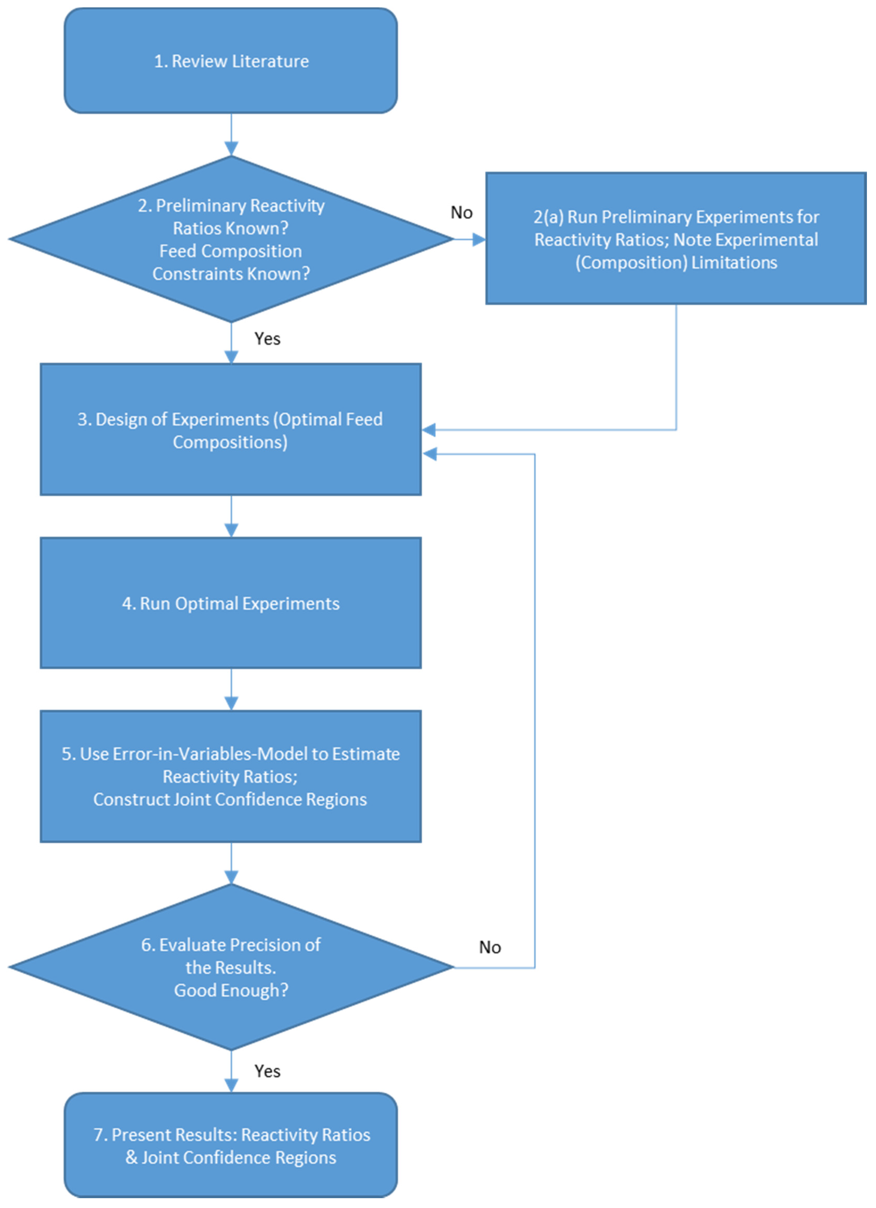
The error-in-variables-model framework, which was outlined in
Figure 1, is applied to the terpolymerization of AMPS/AAm/AAc. This is the first time in the literature that the entire framework, from preliminary investigation and design of experiments to parameter estimation, is verified experimentally.
3.1. Step 1: Review Literature for Polymerization Kinetics
In recent years, several studies have investigated the AMPS/AAm/AAc terpolymer. These have focused on synthesis, characterization, and potential applications for this terpolymer; none of the studies have included terpolymerization kinetics.
For example, Bao et al. [
5] grafted the AMPS/AAm/AAc terpolymer onto sodium carboxymethyl cellulose and montmorillonite (MMT) to create a superabsorbent hydrogel. In this case, physical properties of the synthesized terpolymer (such as degree of swelling, water retention, and morphology) were the focus of the analysis. Similarly, Ma et al. [
6] synthesized the AMPS/AAm/AAc terpolymer via UV irradiation for use as a flocculent. While this group did provide more information about their synthesis steps, the overall focus of the paper was applications. Polymer characteristics including intrinsic viscosity, dissolution time and flocculation performance were presented. This particular terpolymer has also been used in drug-delivery applications [
7]. The drug-delivery system uses superabsorbent polymer composites, so characteristics such as swelling capacity and drug encapsulation efficiency were studied. While the investigation included release profiles for drug-delivery, it did not discuss details surrounding the polymerization kinetics.
In perhaps the most relevant papers to the current work, Peng et al. [
4] and Zaitoun et al. [
3] have studied the AMPS/AAm/AAc terpolymer for petrochemical applications. The work by Peng et al. [
4] describes the free-radical terpolymerization of AMPS/AAm/AAc and its application as a high-temperature resistant filtration control agent. Zaitoun et al. [
3] have investigated the potential to use AMPS/AAm/AAc in enhanced oil recovery (EOR) applications, as the AMPS comonomer is expected to improve shear stability and limit thermal degradation (compared to standard AAm/AAc copolymers). However, in both of these cases, the authors make no mention of polymerization kinetics.
The kinetic characteristics of the terpolymer being synthesized are directly related to its microstructure. Therefore, it is important to have a clear understanding of the terpolymerization kinetics. Since this information is not available in the literature, reliable reactivity ratios for this AMPS/AAm/AAc system will be determined experimentally in what follows.
3.2. Step 2: Determine Preliminary Reactivity Ratios and Establish Feed Composition Constraints
Since, to date, there have been no kinetic studies for this particular terpolymerization in the literature, binary values for the associated copolymer pairs were used as preliminary reactivity ratios. These binary values were obtained experimentally, which allowed for the same experimental set-up to be used for both the co- and terpolymerizations.
For the AMPS/AAm and AMPS/AAc copolymerizations, an in-depth study was recently completed by Scott et al. [
14]. Different reactivity ratio estimates for these copolymers were published previously, but most of these estimates were subject to numerous sources of error (namely, linear parameter estimation techniques for non-linear parameter estimation with no independent replication). In an attempt to provide the most accurate reactivity ratio estimates possible, Scott et al. [
14] used the error-in-variables-model (EVM) technique to design experiments and estimate reactivity ratios for both AMPS/AAm and AMPS/AAc copolymerizations. As an additional advantage, the polymerization conditions (pH, ionic strength, etc.) that were used in these copolymerizations are also used for the terpolymerizations described in the current paper.
Similarly, for the AAm/AAc copolymerization, Riahinezhad et al. [
12] conducted a thorough investigation of the reactivity ratios for this copolymerization system. Again, the same polymerization conditions were used for the AAm/AAc binary system and for the terpolymerizations described in the current paper. Therefore, the reactivity ratios arrived at for the above binary systems can confidently be considered as the “best” binary reactivity ratios for the different pairs. These values are summarized in
Table 1.
One of the advantages associated with EVM is the ability to introduce feed composition constraints on the experimental design. However, since very little kinetic information is available for the AMPS/AAm/AAc terpolymerization, it is difficult to establish whether such constraints exist. In studying the AMPS/AAc copolymer, Scott et al. [
14] reported that the polymerization was extremely slow and minimal precipitate formed when the AAc fraction was high in the feed (
fAAc,0 = 0.85). Similarly, Ryles and Neff [
1] observed that a preliminary feed composition of
fAAc,0 = 0.80 for the AMPS/AAc copolymer made polymer isolation (and subsequent filtering/precipitation) difficult as a result of phase separation. Therefore, for the AMPS/AAm/AAc terpolymer, the feed composition of AAc was constrained such that
fAAc,0 ≤ 0.70.
3.3. Step 3: Apply Design of Experiments to Select Optimal Feed Compositions
The basic idea behind design of experiments is to select optimal feed compositions (experimental trials) which minimize variability in the parameter estimates. As mentioned previously, terpolymerization studies often (incorrectly!) use reactivity ratios extracted from binary systems; based on this analogy, a ternary system is treated as three separate binary copolymerizations. This approach is approximate at best, as it propagates the inherent error present in the binary reactivity ratio estimates, overlooks the effect of the interactions between all three monomers on their reactivity towards each other and is not at all reliable for predicting ternary compositions.
An additional problem with terpolymerization studies is the form of the Alfrey–Goldfinger (A–G) model that is typically used to evaluate instantaneous terpolymerization composition (see Equation (1)). Kazemi et al. [
15] recently showed that selecting different combinations of ratios of mole fractions in the A-G model (e.g.,
F1/F2 and
F1/F3 versus
F1/F2 and
F2/F3) can affect the precision of the reactivity ratio estimates. This work exposed the fact that the model suffers from symmetry issues; final results depend on the arbitrary choice of different combinations of copolymer mole fractions into the parameter estimation scheme. Therefore, in current and future terpolymerization investigations, a recast version of the model (courtesy of Kazemi et al. [
8]) should be used. The recast A–G model presents each instantaneous terpolymer mole fraction as a single response (see Equation (2)). While these expressions may seem more complex than the conventional A–G model, this formulation is symmetrical and error structures are not distorted [
8]:
With this new information in mind, the goal in this step of the procedure is to apply the EVM design criterion to the recast Alfrey–Goldfinger model so that optimal feed compositions (that can lead to the most reliable reactivity ratios) are selected.
EVM considers error in all terms, so using a design of experiments technique within the EVM context helps to account for the error in both the independent variables (feed compositions) and the dependent variables (terpolymer compositions). Details have been presented previously [
8,
9], but the key points are briefly revisited below. The EVM design criterion aims to maximize the determinant of the information matrix (
G), which is the inverse of the variance–covariance matrix of the parameters:
where
ri = number of replicates at the
ith trial (out of n trials),
Zi = vector of partial derivatives of the model function with respect to the parameters (in this case, the partial derivatives of the recast A–G model (Equation (2)) with respect to the reactivity ratios),
Bi = vector of partial derivatives of the model function with respect to the variables (again, in this case, the partial derivatives of the recast A-G model (Equation (2)) with respect to the feed (
f) and terpolymer (
F) compositions), and
V = variance–covariance matrix of the variables (which provides information about measurement error and possible correlation of the variables involved).
As explained in previous work by Kazemi et al. [
9], three optimal experiments are sufficient to estimate terpolymerization reactivity ratios in this nonlinear model scenario. In the terpolymerization problem, the EVM model consists of three equations (see again Equation (2)) and five variables (
f1,
f2,
F1,
F2,
F3); only two of the three feed compositions are independent (
f3 = 1 –
f1 –
f2) and the terpolymer compositions are measured independently. Therefore, for the terpolymerization, there are two independent variables (5 variables – 3 equations = 2) and six (6) parameters (reactivity ratios). The number of optimal experiments needed can be calculated by dividing the number of parameters by the number of independent variables (see Bard [
16] and Duever et al. [
17]); hence, 6 ÷ 2 = 3.
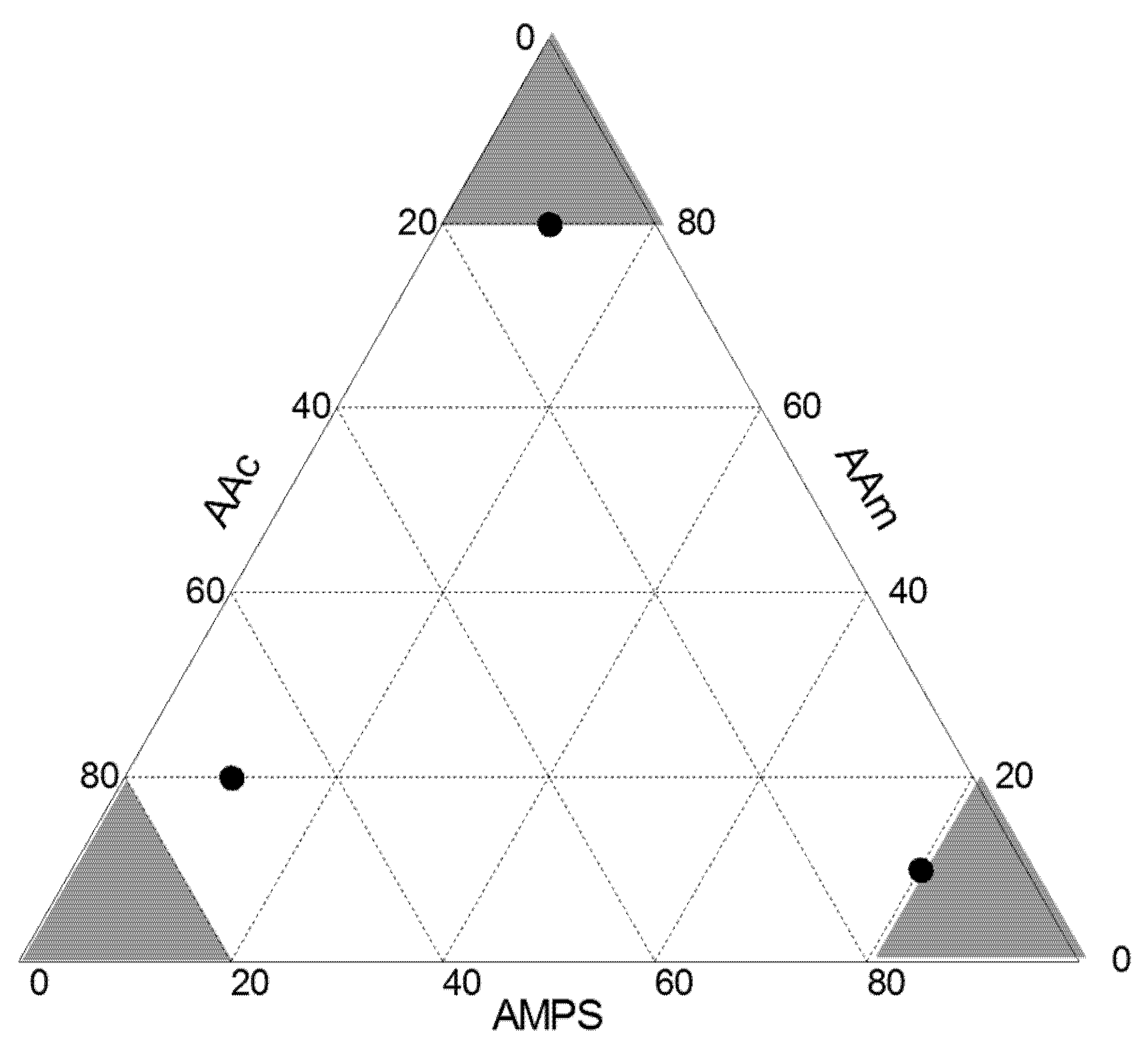
For ternary reactivity ratio estimation, optimal feed compositions are typically located at the corners of the triangular (terpolymerization) composition plot [
9]. To help visualize the location of the optimal feed compositions for this system,
Figure 2 combines the “suboptimal” regions (shaded areas) as well as the three optimal points located close to or inside these regions. Polymerizations run using these three optimal feed compositions (recipes) will provide sufficient information for reliable reactivity ratio estimation.
3.4. Step 4: Perform Experiments; Collect Conversion and Composition Data
3.4.1. Low Conversion Experiments
The first attempt at estimating the reactivity ratios for the AMPS/AAm/AAc terpolymerization was conducted by analyzing low conversion data, similar to the conventional approaches for estimating reactivity ratios of copolymerizations and terpolymerizations [
9,
18]. As shown in
Table 2, the three feed compositions correspond to the optimal feed compositions of
Figure 2 (reflecting also process constraints), and the experimental data were limited to low conversion (
Xw < 0.100). Conversion values with a “*” indicate results from an independently replicated polymerization; the same classification will be used in
Table 3. That is, these replicates were synthesized entirely independently, using freshly made solutions, etc. Conversion was determined again using gravimetry, and samples were independently characterized using elemental analysis, as described in
Section 2.4. Note also that experimental data in
Table 2 and
Table 3 are presented in terms of mass conversion (
Xw), which should not be confused with molar conversion (
Xn; see, for example, Equations (4) through (6)).
Since the conversion level was kept low for these runs, it can be assumed that the composition drift is negligible. Therefore, the instantaneous terpolymer composition model (that is, the recast Alfrey–Goldfinger model, Equation (2)) and the EVM parameter estimation technique were employed [
9]. Details regarding the parameter estimation technique, the resulting reactivity ratio estimates, and the corresponding joint confidence regions (JCRs) will be presented in Step 5 (
Section 3.5).
3.4.2. Medium-High Conversion Experiments
The recast A–G model (Equation (2)) is a significant improvement over Equation (1), but it is only valid for low conversion data sets. In order for copolymer composition drift to be negligible (that is, for the initial feed composition to remain unchanged and for the (measurable) cumulative copolymer composition to be equal to its instantaneous value), experimental data must be collected at very low conversion levels. This restrictive assumption introduces additional sources of error, including significant experimental difficulties.
As an alternative, a cumulative ternary composition model has been considered in order to estimate ternary reactivity ratios using the full conversion trajectory. The cumulative model (essentially the Skeist equation applied to terpolymerization), shown in Equation (4), relates the cumulative terpolymer composition for each monomer (
) to the initial mole fraction of monomer in the feed (
fi,0), and the corresponding mole fraction of unreacted monomer (
fi) and molar conversion (
Xn):
In this step of the procedure, reactivity ratios for the AMPS/AAm/AAc terpolymerization were estimated using the same optimal feed compositions of
Figure 2, but this time running the terpolymerizations to medium-high conversion levels (see
Table 3). Since it is no longer valid to assume constant composition (that is, composition drift is no longer negligible),
fi must be evaluated over conversion
Xn, according to the model in ordinary differential equation form, shown in Equation (5) (where
Fi values are calculated using Equation (2)). Given the initial conditions
fi =
fi,0 at
Xn = 0, a numerical solution can be used to evaluate terpolymer compositions along the full conversion trajectory:
It is important to note that molar conversion (
Xn) is used in both Equations (4) and (5), but that mass conversion (
Xw) is reported in the experimental data tables (see
Table 2 and
Table 3). Molar conversion and mass conversion are related using monomer molecular weights (
MWi), as shown in Equation (6):
This methodology (using direct numerical integration (DNI) to evaluate the cumulative composition model) has been described previously by Kazemi et al. [
8]. The current approach (i.e., integrating the instantaneous terpolymer composition model (Equation (2)) over conversion via Equations (4) and (5) and conducting parameter estimation via EVM simultaneously) is generally preferable for parameter estimation, as it includes all available information from the system (not only at low conversion as per typical approaches), and does not suffer from the limiting assumptions or experimental difficulties associated with low conversion data analysis. As was the case for the low conversion experiments, estimation details along with reactivity ratio estimates and corresponding JCRs will be shown in Step 5 (
Section 3.5).
3.5. Step 5: Use EVM to Estimate Reactivity Ratios; Construct Joint Confidence Regions
The error-in-variables-model (EVM), described previously for the design of experiments (see
Section 3.3), can also be used in the current parameter estimation step. EVM is one of the most powerful non-linear regression approaches available, as it considers all sources of experimental error (both in the independent and dependent variables) [
19]. EVM not only forces the experimenter to consider all sources of error, but also provides estimates of the true values of other variables involved in the model along with the parameter estimates. Therefore, it is by far the most statistically correct and comprehensive approach for reactivity ratio estimation [
20].
In this step, the EVM approach is used to estimate reactivity ratios for both the low and medium-high conversion data. However, as discussed in
Section 3.4, the terpolymerization model differs for each data set: low conversion data are analyzed using the recast instantaneous terpolymerization model (Equation (2)) along with the related low conversion assumptions, whereas the medium-high conversion data are analyzed with the direct numerical integration (DNI) of the instantaneous model, i.e., using the cumulative composition model (see Equations (2), (4) and (5)). The nested-iterative EVM implementation has been described in detail in several previous references (for instance, see references [
8,
9,
10,
17,
18,
21,
22] cited herein), so no further details will be presented.
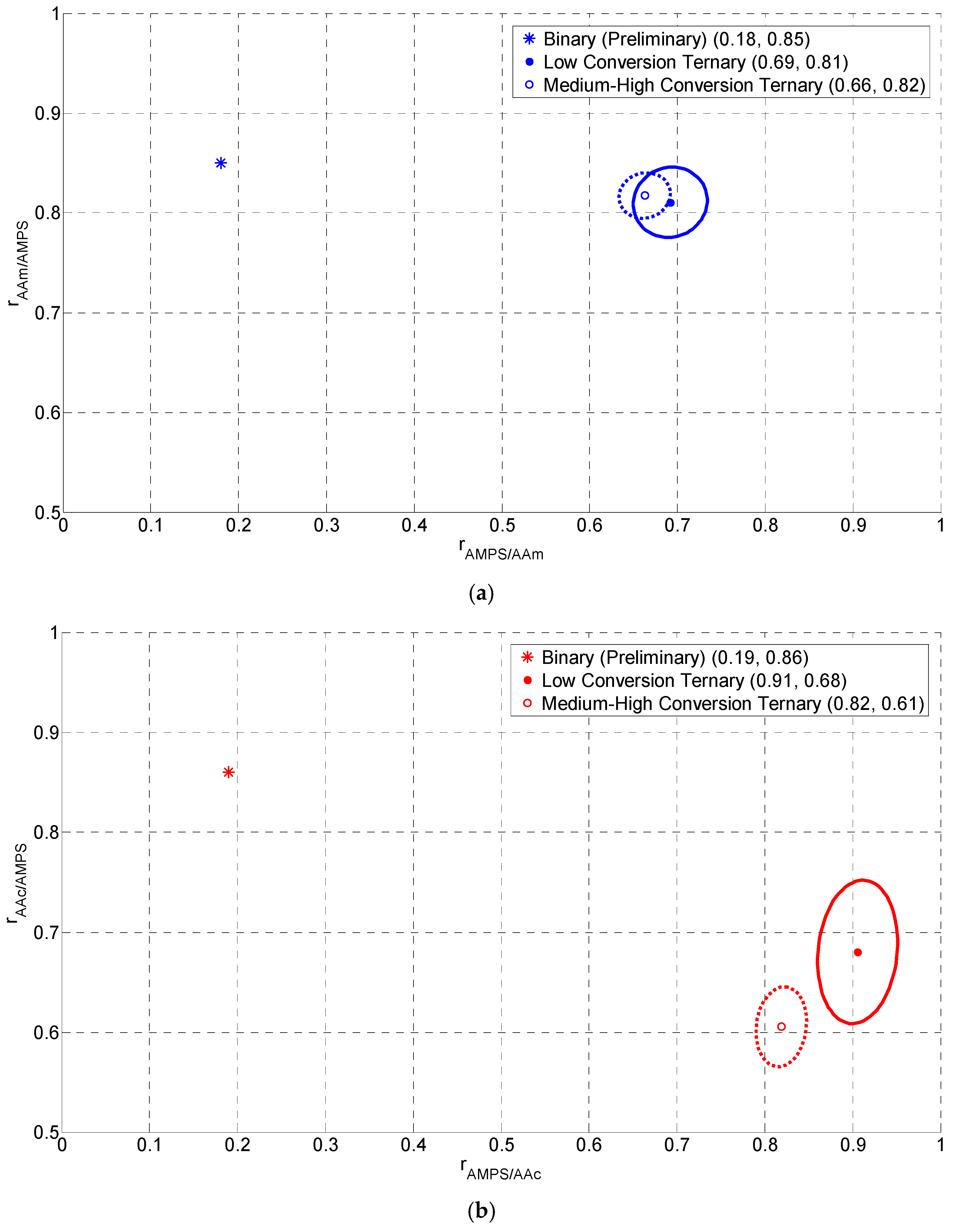
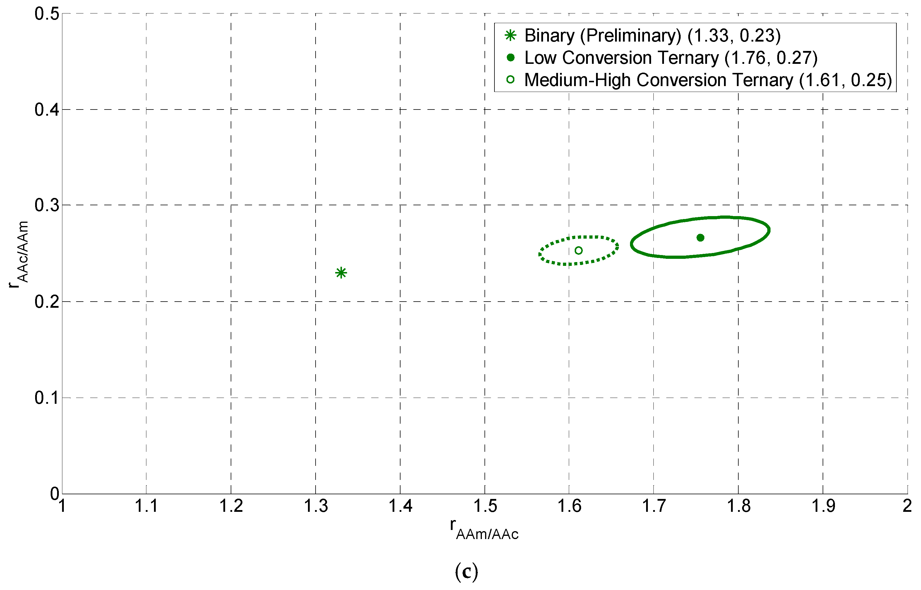
The terpolymerization reactivity ratio estimates and corresponding JCRs for both data sets (
Table 2 and
Table 3), along with the corresponding binary (copolymerization) reactivity ratios (
Table 1) are presented in
Figure 3. In all cases, the results show that JCRs from medium-high conversion data are smaller (and therefore more precise) than JCRs from low conversion data. These results are as expected; utilizing all of the experimental information available and eliminating potentially inaccurate assumptions can improve the precision of the point estimates. These results confirm (for the first time) that EVM can successfully be used to analyze directly experimental data from terpolymerizations over the whole conversion range. In addition, the results prove that three optimally designed ternary feed compositions can provide sufficient information to estimate reactivity ratios with very little correlation for this terpolymerization system, as one can realize from the orientation of the JCRs. In addition, in all cases, the literature binary reactivity ratio estimates are located outside the terpolymerization JCRs.
3.6. Step 6: Decide Whether Results Are Precise Enough
In Step 5 (
Section 3.5), the reactivity ratio estimates and associated JCRs confirm that the EVM-based experimental design and parameter estimation method for ternary systems work very well with experimental data directly from the AMPS/AAm/AAc terpolymerization. The reliability of the results is first established by examining the size of the JCRs and by noting the lack of correlation between the parameters (see
Figure 3).
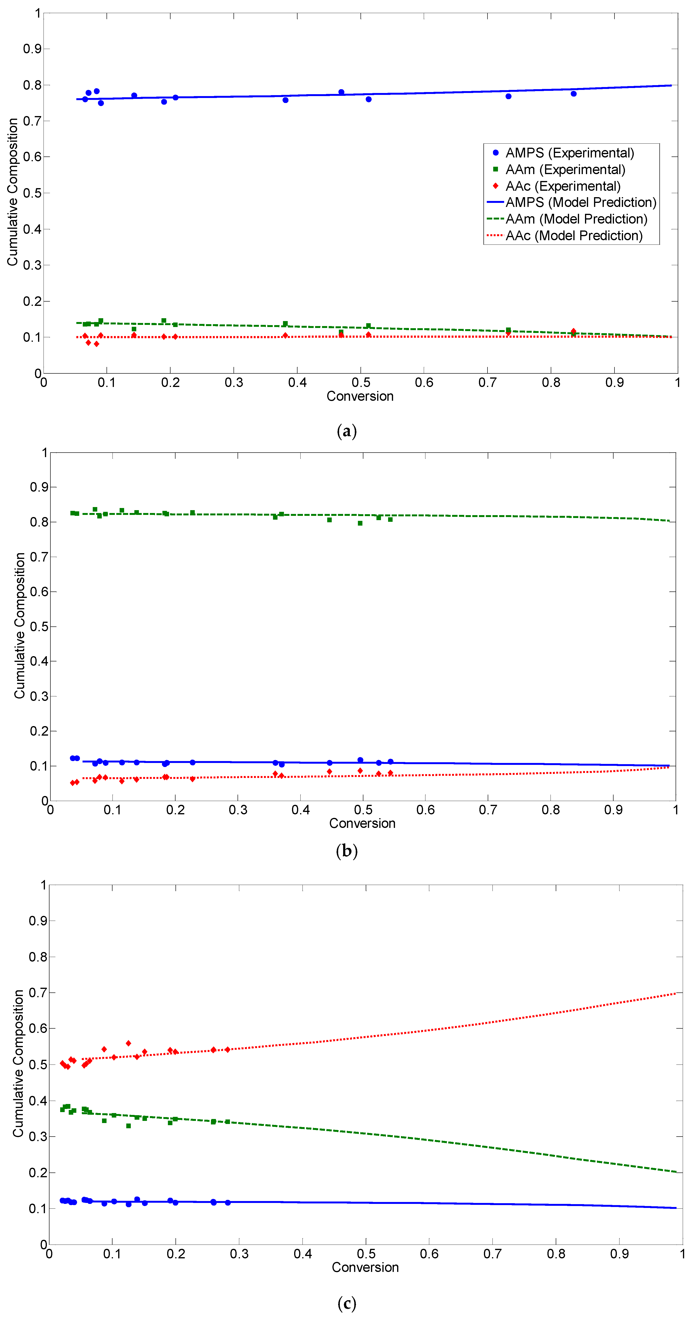
In the second diagnostic stage, it is important to investigate the accuracy of the reactivity ratios by running additional checks. One of the most common diagnostic checks is to evaluate the behavior/profiles of the cumulative terpolymer composition. Model predictions (using reactivity ratio estimates) for the terpolymer composition over the polymerization trajectory are compared to experimentally measured terpolymer compositions. An acceptable agreement between predicted and experimental results reflects the reliability and accuracy of the reactivity ratios for the terpolymerization system.
Thus, direct numerical integration (DNI) was applied to the recast version of the instantaneous terpolymer composition equation (see Equation (2)) using newly determined reactivity ratio estimates. Since the medium-high conversion data provided more information (and smaller JCRs), the reactivity ratios estimated from the data of
Table 3 were used. The predicted cumulative terpolymer composition trajectories versus conversion, as well as the experimental points obtained via elemental analysis, are shown in
Figure 4 for all three of the optimally designed feed compositions.
Figure 4 shows that, in all three cases, the predicted terpolymer composition trajectories (from ternary reactivity ratio estimates) capture the experimentally observed behavior satisfactorily. At low conversion, however, there are some minor discrepancies between the model and the experimental results. The noise seen in the experimental data is typical at such low conversions, which confirms the need for higher conversion experiments. Thus, in spite of the natural variation in experimental results, it is possible to conclude that the cumulative terpolymer composition (DNI) model and the EVM-based estimated ternary reactivity ratios can successfully predict the behavior of the system. This is an important diagnostic check for this system (and for terpolymerization studies, in general), as it indicates that employing the terpolymerization composition model and the EVM framework leads to precise and reliable reactivity ratios for the system.
3.7. Step 7: Present Reactivity Ratios and JCRs
It was shown in Step 5 (
Section 3.5) that using medium-high conversion data provides smaller joint confidence regions (JCRs) for reactivity ratio estimation (compared to conventional low conversion data analysis). In addition, in Step 6 (
Section 3.6), the reactivity ratio estimates from medium-high conversion data were successfully used to predict the cumulative terpolymer composition. Therefore, of the reactivity ratio estimates presented in
Table 4, the information in the last row (for ternary reactivity ratio estimation of medium-high conversion data) is the most precise. The JCRs associated with these estimates have been presented previously in
Figure 3.


