Nonlinear Flow Characteristics of a System of Two Intersecting Fractures with Different Apertures


1
State Key Laboratory for Geomechanics and Deep Underground Engineering, China University of Mining and Technology, Xuzhou 221116, China
2
School of Engineering, Nagasaki University, 1-14 Bunkyo-machi, Nagasaki 8528521, Japan
3
State Key Laboratory of Mining Disaster Prevention and Control Co-Founded by Shandong Province and the Ministry of Science and Technology, Shandong University of Science and Technology, Qingdao 266510, China
*
Author to whom correspondence should be addressed.
Processes 2018, 6(7), 94; https://doi.org/10.3390/pr6070094
Submission received: 27 June 2018
/
Revised: 11 July 2018
/
Accepted: 12 July 2018
/
Published: 20 July 2018
(This article belongs to the Section Advanced Digital and Other Processes)
Abstract
:The nonlinear flow regimes of a crossed fracture model consisting of two fractures have been investigated, in which the influences of hydraulic gradient, surface roughness, intersecting angle, and scale effect have been taken into account. However, in these attempts, the aperture of the two crossed fractures is the same and effects of aperture ratio have not been considered. This study aims to extend their works, characterizing nonlinear flow through a system of two intersecting fractures with different apertures. First, three experiment models with two fractures having different apertures were established and flow tests were carried out. Then, numerical simulations by solving the Navier-Stokes equations were performed and the results compared with the experiment results. Finally, the effects of fracture aperture on the critical pressure difference and the ratio of hydraulic aperture to mechanical aperture were systematically analyzed. The results show that the numerical simulation results agree well with those of the fluid flow tests, which indicates that the visualization techniques and the numerical simulation code are reliable. With the increment of flow rate, the pressure difference increases first linearly and then nonlinearly, which can be best fitted using Forchheimer’s law. The two coefficients in Forchheimer’s law decrease with the increasing number of outlets. When increasing fracture aperture from 3 mm to 5 mm, the critical pressure difference increases significantly. However, when continuously increasing fracture aperture from 5 mm to 7 mm, the critical pressure difference changes are negligibly small. The ratio of hydraulic aperture to mechanical aperture decreases more significantly for a fracture that has a larger aperture. Increasing fracture aperture from 5 mm to 7 mm, that has a negligibly small effect on the critical pressure difference will however significantly influence the ratio of hydraulic aperture to mechanical aperture.
1. Introduction
The assessment of hydraulic properties of deep fractured rock masses has attracted attention in many fields, such as CO2 sequestration [1,2], enhanced oil recovery [3,4], and groundwater use [5,6,7,8,9]. In tight rocks (i.e., granite and basalt), the permeability of fractures is much larger than that of the rock matrix, and as a result, the rock matrix is assumed to be impermeable [10,11,12,13]. This assumption is commonly adopted when calculating the permeability of highly fractured rock masses using modelling techniques such as discrete fracture network (DFN) models [14,15,16]. Another assumption is that the fluid flow through fractures is in the linear regime and follows the cubic law in which the flow rate is linearly proportional to the pressure difference [10,17,18,19,20]. However, in the high-pressure packer tests and/or karst systems, the fluid flow is in the nonlinear regime where the cubic law is not suitable [21,22]. In such a case, the permeability/conductivity of a fractured rock mass will be underestimated when still using the cubic law [21]. Therefore, the nonlinear flow characteristics of fractured rock masses should be investigated.
The nonlinear flow regimes through single fractures that are the simplest element of the complex fracture networks, have been extensively studied in the previous works. It has been found that rougher fractures can more significantly increase the length of flow paths and induce energy losses, which subsequently decreases the permeability [23,24]. Some studies have shown that the contact including contact ratio and contact shape can robustly change the tortuosity and flow paths of fluid, and then influence the nonlinear flow properties [25,26]. Since the rock masses are commonly moved along a fault when an earthquake occurs, the effect of shear displacement on the onset of nonlinear flow has been estimated both experimentally and numerically [27,28,29,30]. Besides the nonlinear flow through single fractures, the fracture interaction is another main cause for the nonlinear flow because the fluid redistributes at the interaction. Kosakowski and Berkowitz [21] depicted that the fluid flow transits from the linear regime to the nonlinear regime when Re > 10, by numerically solving the complex Navier-Stokes equations. The influences of hydraulic gradient, surface roughness, intersecting angle, and scale effect on the nonlinear flow characteristics at the intersections have been both experimentally and numerically investigated [31,32,33]. They found that the nonlinearity can be negligible when the ratio of fracture aperture to fracture length is smaller than 0.001, and the hydraulic gradient that is less than 0.001 plays a sufficiently small role on the nonlinear flow. However, in these attempts, the aperture of the two crossed fractures is the same and effects of aperture ratio have not been considered, if any. According to the cubic law, the flow rate through the fracture is linearly proportional to the cube of aperture [34]. A small variation in fracture aperture can induce a significant change in the flow rate. Many previous studies have contributed to the investigations of effect of fracture aperture distribution on the macroscopic flow rate through complex fracture networks [10,35,36], while other studies focused on the fracture aperture distribution [37,38,39] and linked it with fracture length [40,41,42,43,44,45,46]. Therefore, fracture aperture is a very important parameter that dominates the fluid flow. For a system of two intersecting fractures that is a simple fracture network, the aperture ratio of the two fractures would also be of special importance for investigating the hydraulic properties such as nonlinear flow regimes.
The present study extends the works of Li et al. [32] and Wu et al. [33] to study the nonlinear flow properties of a crossed fracture model consisting of two fractures with different apertures. First, three experiment models, with two fractures having different apertures, were established and flow tests were carried out. Then, numerical simulations by solving the Navier-Stokes equations were performed and the results compared with the experiments, which verified the validity of the simulation. Finally, the effects of fracture aperture ratio on the critical pressure difference and the ratio of hydraulic aperture to mechanical aperture were systematically analyzed.
2. Theoretical Background
The flow of incompressible steady Newtonian fluid is governed by the Navier-Stokes equations, written as [47]:
where u is the flow velocity tensor, ρ is the fluid density, P is the hydraulic pressure, T is the shear stress tensor, t is the time, and f is the body force tensor. For a laminar flow in single fractures, the convective acceleration terms, , are the only source of nonlinearity, which are strongly affected by the geometries of void spaces resulting from complex surface roughness of fractures [48]. When the flow rate is sufficiently small, the Navier-Stokes equations can reduce to the cubic law, in which the flow rate is linearly proportional to the pressure gradient and is commonly adopted when simulating fluid flow in complex fracture networks [14,49,50], as follows:
where Q is the flow rate, w is the fracture width, e is the hydraulic aperture, μ is the dynamic viscosity, and is the pressure gradient.
Note that Equation (2) is applicable when the flow rate is sufficiently small. When the flow rate is large (i.e., Re > 10), the Q is no longer linearly proportional to [51]. For describing the nonlinear relationship between Q and , the famous Forchheimer’s law is proposed as [34,52,53]:
where A and B are two coefficients that represent the linear and nonlinear terms, respectively.
The E contributes to the ratio of pressure drop caused by the nonlinear term to the total pressure drop. Many critical values have been assigned to E to quantify the onset of nonlinear flow, such as E = 0.01 [55], 0.05 [56], and 0.1 [28,51], among which E = 0.1 is the most adopted and is used in the present study.
3. Flow Testing System
3.1. Specimen Preparation
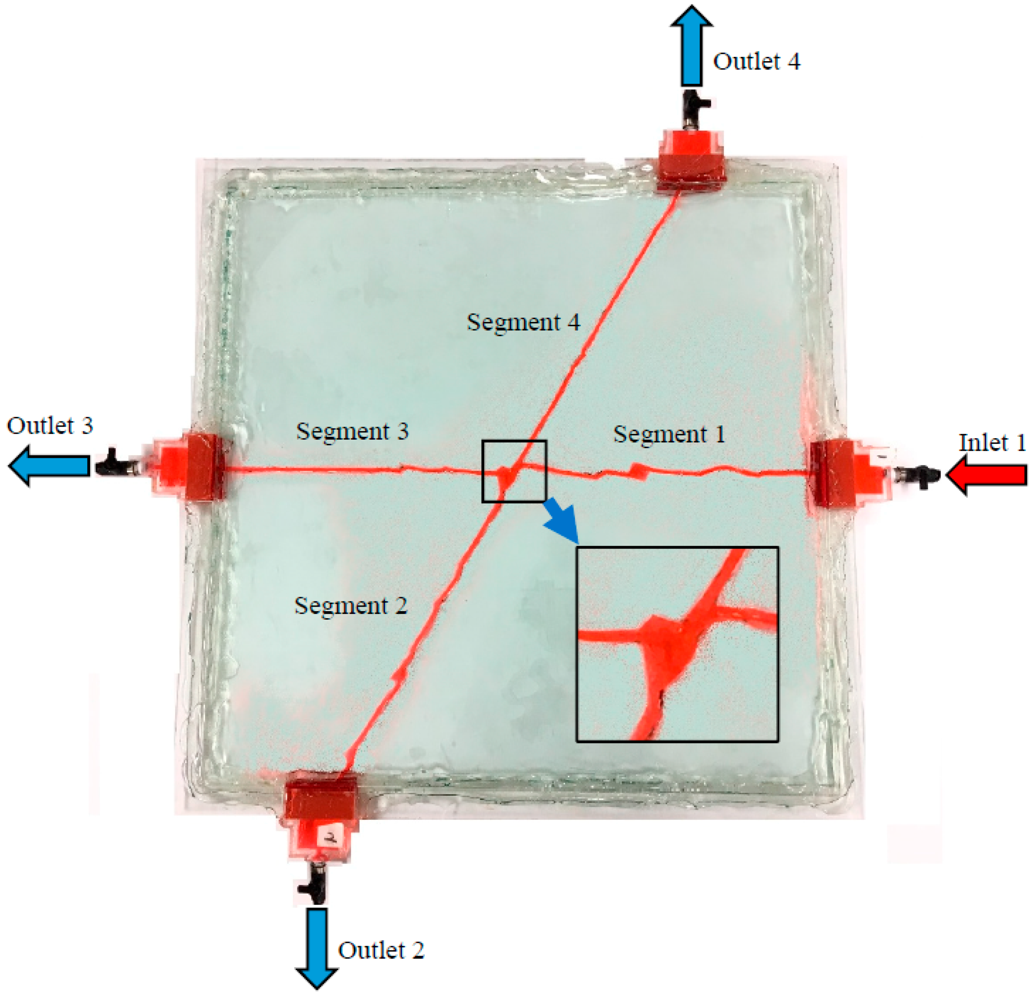
One glass plate that has a size of 50 cm × 50 cm × 0.5 cm was cut into two parts in which there are two intersected fractures as shown in Figure 1. The intersecting angle of the two fractures is 60 degrees. Since the glass is a brittle material, the fractures deviated from the pre-designed sketch, resulting in rough fracture surfaces. During the cutting, some parts of the glass were damaged and removed from the model, making the two walls of a fracture ill-mated. This is also commonly observed in nature, for example, in shallow rock masses where mineral dissolution occurs [57]. The mean mechanical aperture (E0) of each fracture was designed by shifting a separated glass plate. However, the shifting was handled by hand. Therefore, the accurate E0 should be calculated again after the model is manufactured. The dye solute was injected into the model and then all the inlet and outlets were closed. A high-resolution charged coupled device (CCD) camera (Optem Inc., New York, NY, USA) was then utilized to capture each part of the model. Finally, the geometries of the fractures were re-plotted in AutoCAD. As a result, three experimental models (Cases 1–3) were made; their geometries included tortuous segment length (Lt), aperture, and surface roughness and are shown in Table 1, in which the mechanical aperture is represented by E0 and fracture surface roughness is represented by root-mean-square of first derivative of asperity height, Z2, and is calculated using the following equation [58,59]:
where xi and zi are the coordinates of the fracture surface profile, and M is the number of sampling points along the length (i.e., x coordinate) of a fracture.
3.2. Test System
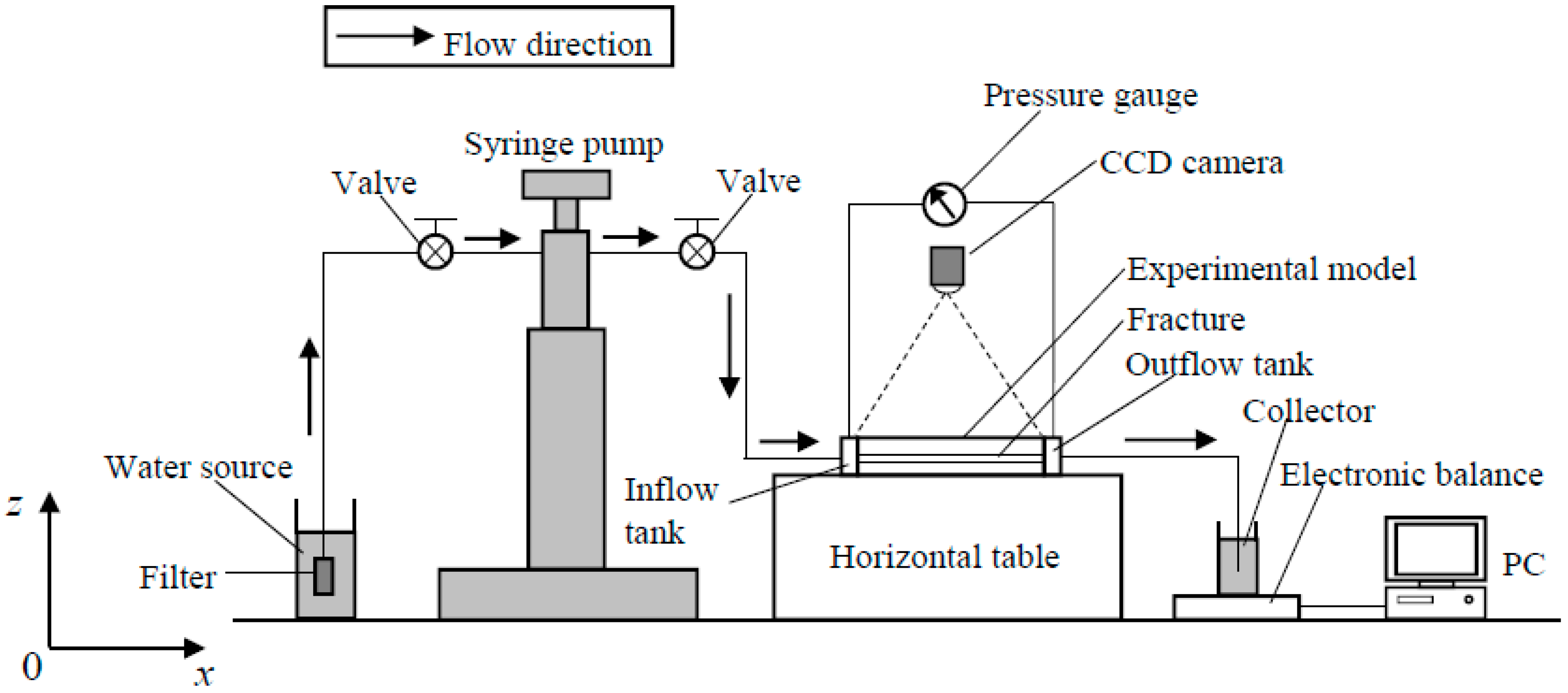
Figure 2 shows the experimental system of the fluid flow test. The fluid was first stored in a syringe pump with an accuracy of ±0.001 mL/min. Then the valve in the left side of the syringe pump was closed and that in the right side of the syringe pump was opened. The fluid was then injected into the model with a fixed flow rate. The pressure difference between the inlet and outlet was measured using a differential pressure gauge with an accuracy of ±10 Pa. The fluid out of the model was collected using a collector; its weight was measured using an electronic balance with an accuracy of ±0.01 g and was recorded in a computer that was linked with the electronic balance using a R232 data line.
It is assumed that the fluid is pure water and the density is 998.2 kg/m3 at a room temperature 20 °C. The dynamic viscosity is 0.001 Pa·s. The glass is impermeable and fluid only flows along the connected fractures.
3.3. Test Procedure
Before the test, all the inflow and outflow tanks, tubes, and fractures were filled with water. The air bubbles within them were removed using a vacuum pump. Although there were four tanks, only one tank was used as the inflow tank and the other three tanks were used as the outflow tanks. For each model, six cases were tested in which the combinations of outlets were different, including outlet 2, 3, 4, 2 and 3, 2 and 4, 2 and 3 and 4. The flow rate of fluid from the syringe pump was set varying from 0 to 100 mL/min. When the fluid flow was in the steady state, the pressure difference between the inlet and outlet was recorded. Finally, the flow rate–pressure difference (Q~ΔP) curves were plotted.
4. Numerical Models and Flow Calculation
4.1. Numerical Models and Meshing
To verify the validity of the visualization technique used for obtaining fracture geometries, three numerical models were established by replotting the geometries of experimental models corresponding to Cases 1–3 in Table 1. The three numerical models have the same model lengths and fracture geometries such as aperture and fracture surface roughness with those of experimental models. However, as shown in Table 1, the apertures of the segments of fractures for Cases 1–3 are different and do not show some rules, which therefore cannot be utilized for parametric study. To solve this issue, we subsequently established another three numerical models and their enlarged views of intersection are shown in Figure 3. The fracture surface roughness and segment length are the same as those in the Cases 1–3, but the apertures of the fractures are different as tabulated in Table 1. The apertures of segments 1 and 3 are fixed as 3 mm, yet the apertures of segments 2 and 4 are changed from 3 mm (see Figure 3a), to 5 mm (see Figure 3b), and to 7 mm (see Figure 3c), respectively.
The numerical models were plotted using software AutoCAD (Autodesk Inc., California, United States, AutoCAD2010), and were then exported in the sat file format. Software Gambit (Fluent Inc., New York, NY, USA, Gambit2.4.6) was used for meshing using hexahedral cells. An interval of approximately 0.5 mm was set. As a result, the total number of hexahedral cells for the six cases ranged from 212,320 to 323,060 due to the difference in fracture aperture. Finally, the stored file from Gambit was imported into finite volume method (FVM) software FLUENT for flow calculation, in which the Navier-Stokes equations were solved. For the fracture aperture, we chose values of 3–7 mm, which is much larger than that in practical engineering. This is because the meshing number (or number of hexahedral cells) should be one hundred times larger than the current models (with number of hexahedral cells varying from 212,320 to 323,060 as shown in Table 1), if the fracture aperture range from 0.3–0.7 mm and the same number (i.e., about 6 in the present study) of layer is kept along the aperture direction. Using a common computer, this meshing cannot be generated and the fluid flow cannot be efficiently modeled by solving the Naver-Stokes equations. Considering this, the magnitude of fracture aperture that is several millimeters should be accepted.
4.2. Boundary Conditions and Flow Calculation
Assumptions were made that the rock matrix would be impermeable with fluid flowing along connected fractures. Therefore, a constant hydraulic pressure was applied on the inlet and the outlet connected to the air, and the flow rate from the outlet was recorded. For each case in Table 1, the fluid flowed through the model from inlet (inlet 1) to outlet (i.e., outlet 2, 3, 4, 2 and 3, 2 and 4, and 2, 3 and 4). The calculated Q~ΔP curves for Cases 1–3 were compared with those of experimental results, and the calculated Q~ΔP curves for Cases 4–6 were used for deep analysis.
5. Results and Analysis
5.1. Comparison between Flow Tests and Numerical Simulations
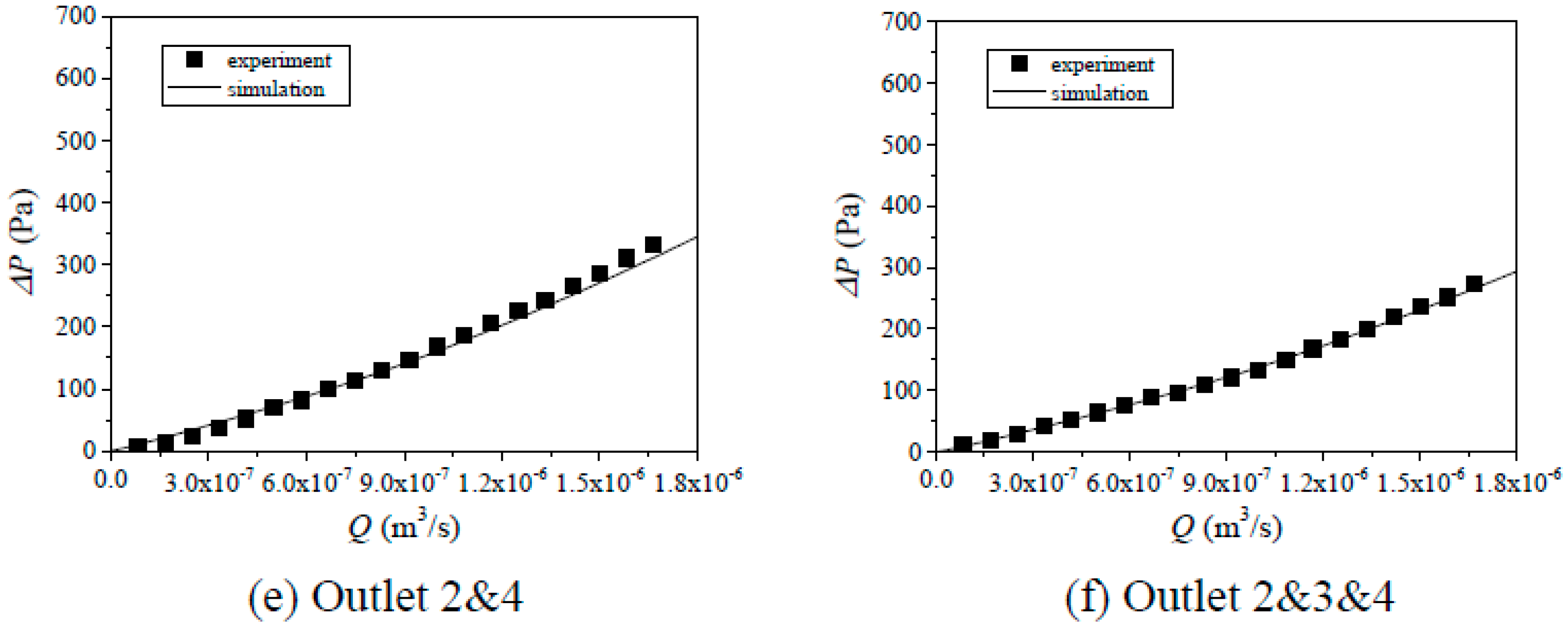
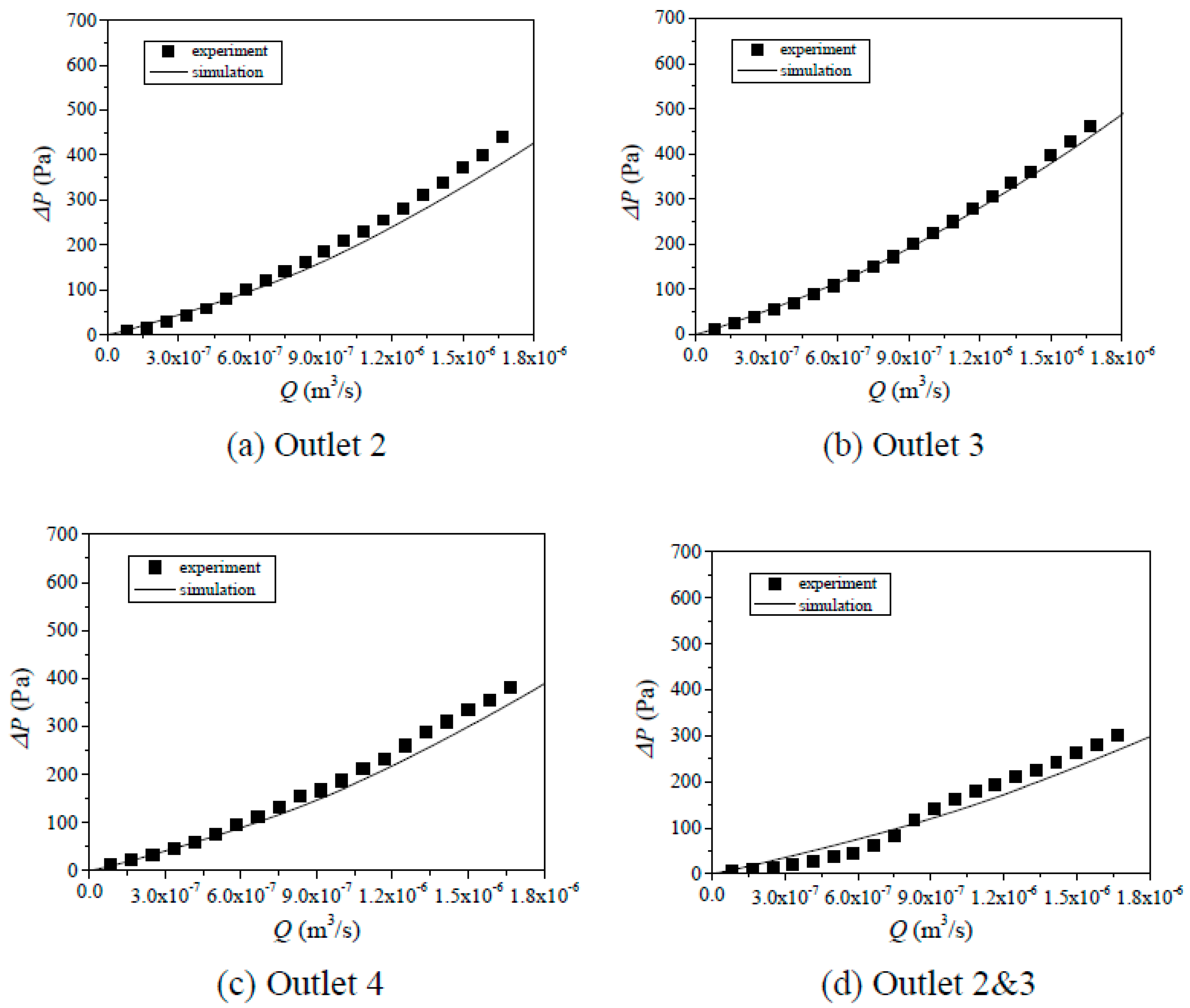
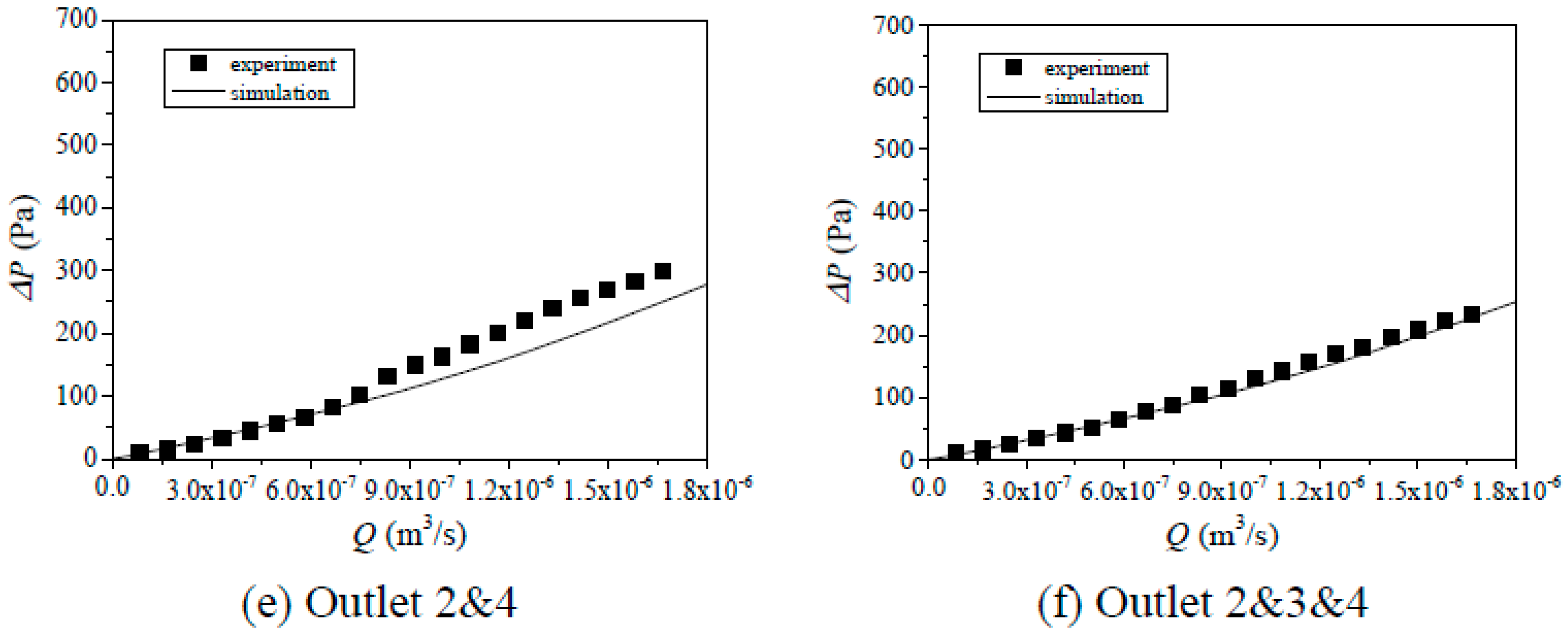
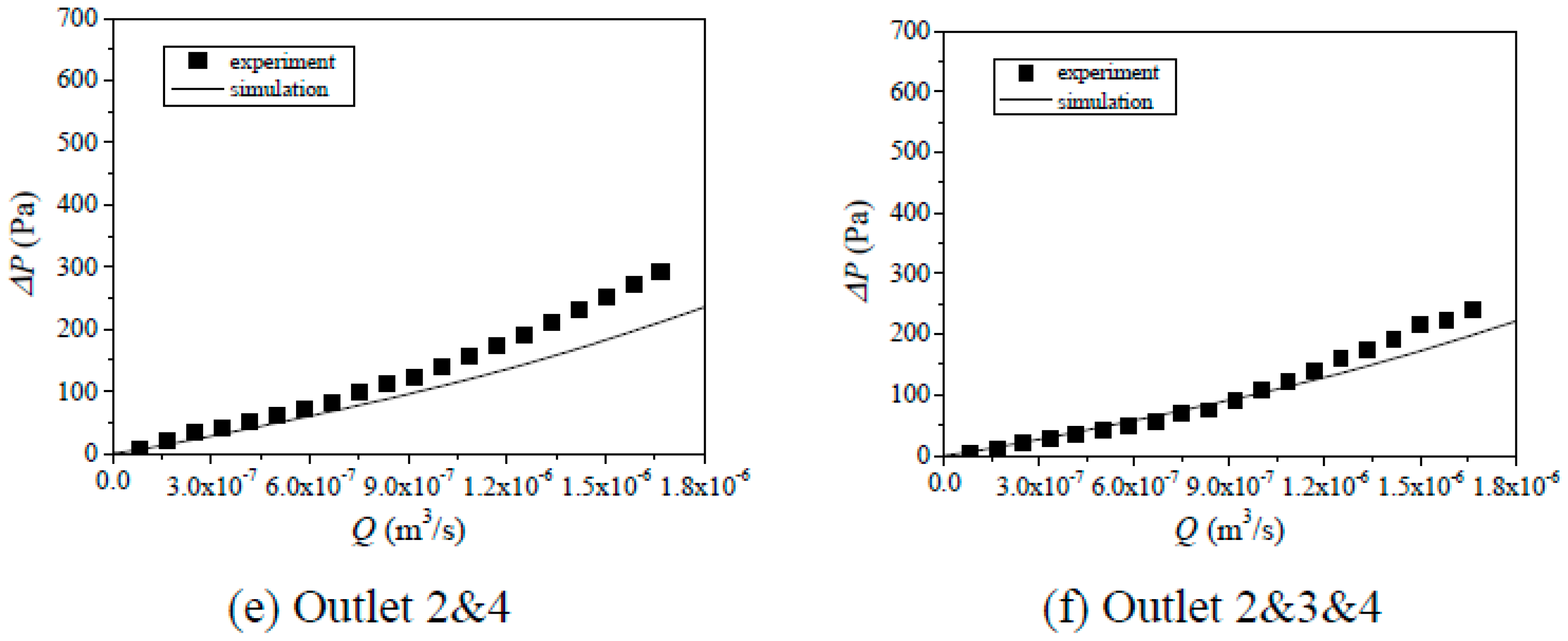
Since the geometries of the models used in flow tests and numerical simulations for Cases 1–3 in Table 1 were the same, their results, such as the Q~ΔP curves with different combinations of outlets (i.e., outlet 2, 3, 4, 2 and 3, 2 and 4, and 2 and 3 and 4) were compared as shown in Figure 4, Figure 5 and Figure 6. Both results show that with the increment of Q, ΔP increases first linearly and then nonlinearly. This is because when the Q is small, the inertial effects can be negligible and fluid flow obeys the cubic law (see Equation (2)), in which Q is linearly proportional to ΔP. When the Q is large, the inertial force is significantly large with respect to the viscous force and it cannot be negligible. As a result, with continuously increasing Q, ΔP increases nonlinearly versus Q (see Equation (3)) and the increasing rate of ΔP increases due to energy losses induced by eddies. With the increase in the number of outlets, for examples from 1 outlet (outlet 2, 3, or 4) to 3 outlets (outlets 2 and 3 and 4), for the same Q, ΔP decreases. A possible reason is that the more outlets correspond to the larger flow volume, and as a result, the ΔP decreases according to Darcy’s law. Even though the simulated results agree well with the tested results in a whole such as Figure 4c,e,f, Figure 5b,f and Figure 6b,c, their results deviate for some cases such as Figure 4a,b and Figure 6a,c, in which the calculated ΔP is either underestimated (Figure 4a) or overestimated (Figure 4b). The deviations arise from the model manufacture in which the glass was not cut strictly along the z-direction as shown in Figure 1 and there existed an angle between the destroyed direction and the z-direction. Thus, in AutoCAD, only the surface of the fractures can be replotted and the void space of fractures along the z-direction cannot be accurately characterized. As a result, the geometries of the fractures in the numerical models are slightly different from those in the experimental models.
5.2. Parametric Studies
In this section, parametric studies are performed using the numerical models as shown for Cases 4~6 in Table 1, in which the aperture of one fracture is fixed as 3 mm and the aperture of another fracture varies from 3 mm, to 5 mm, and to 7 mm, respectively, but their intersecting angle is still fixed as 60 degrees.
5.2.1. Effect of Fracture Aperture on Q~ΔP Curves
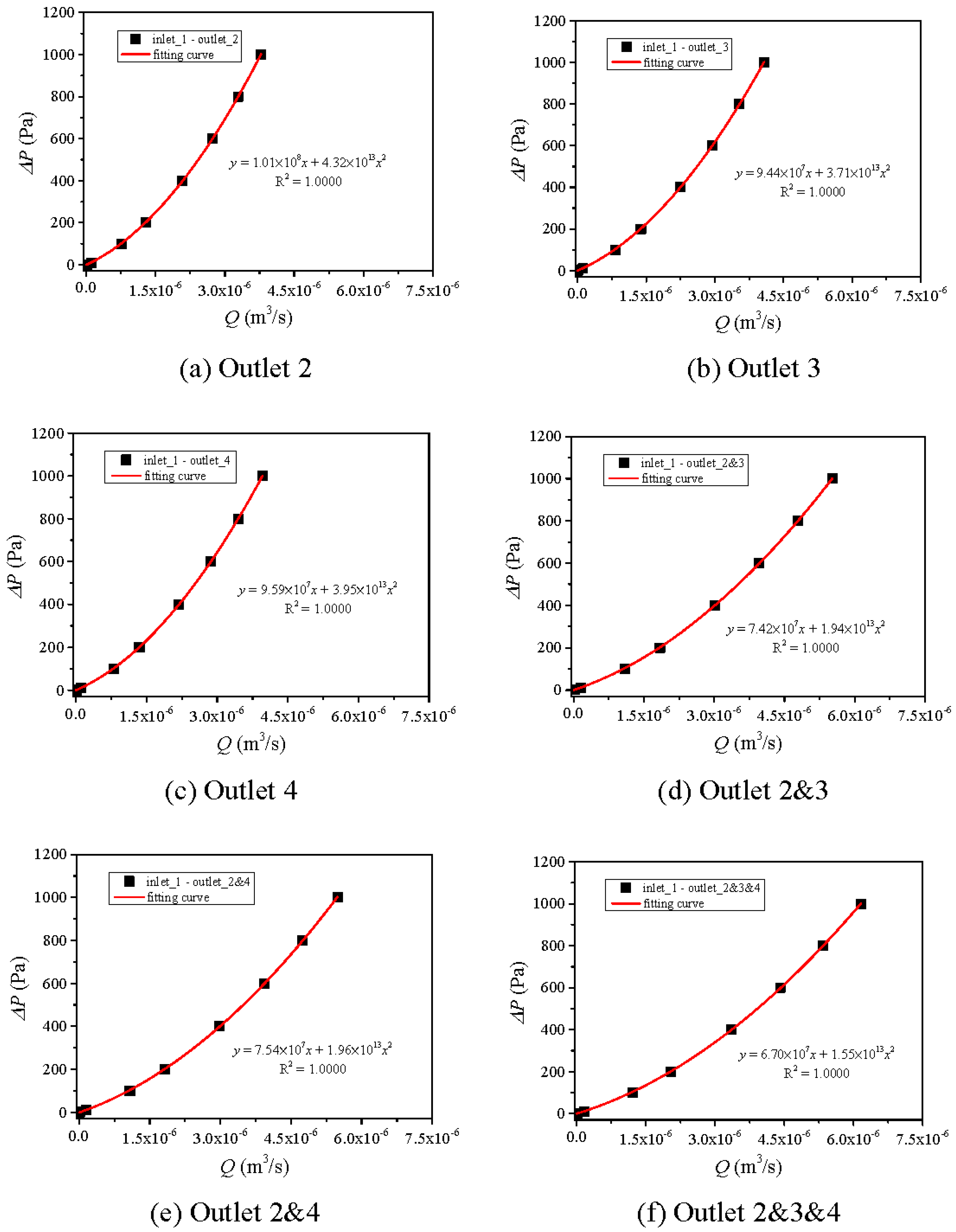
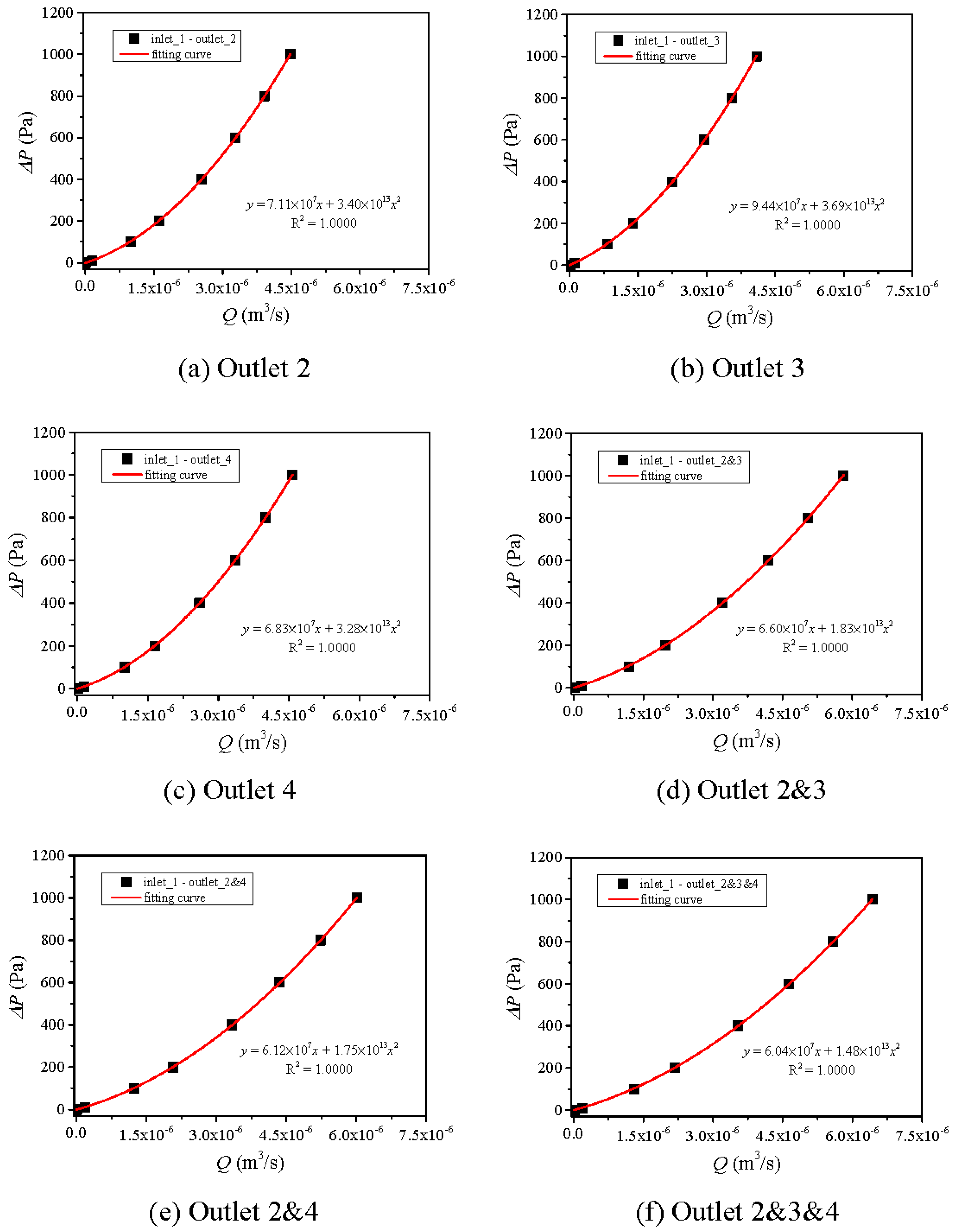
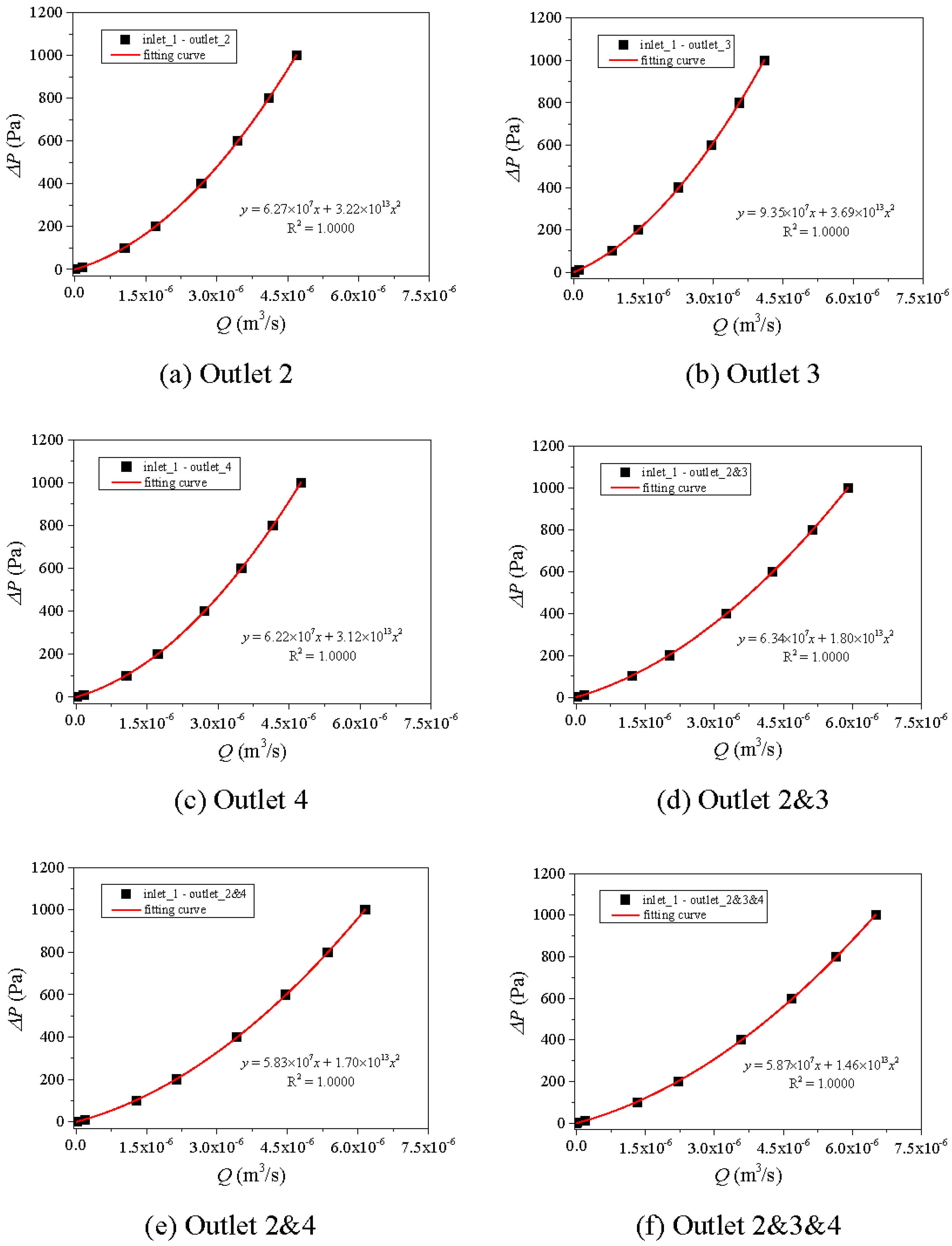
Figure 7, Figure 8 and Figure 9 present the Q~ΔP curves with varying ΔP from 0 to 1000 Pa. With the increment of Q, ΔP increases nonlinearly, and their relationships can be fitted using a zero-intercept quadratic equation as shown in Equation (3). The larger Q, the larger increasing rate of ΔP. This indicates that the larger the flow rate, the stronger the nonlinearity of fluid flow. With increasing the number of outlets, for examples from 1 outlet (outlet 2, 3, or 4) to 2 outlets (outlet 2 and 3 or 2 and 4), or to 3 outlets (outlet 2 and 3 and 4), the curves move rightwards and both the coefficients A and B in Equation (3) decrease. For the cases with the same number of outlets (i.e., outlet 2, 3, and 4), the Q~ΔP curves and coefficients A and B are close to each other, indicating that when the flow volume is in the same order of magnitude, the hydraulic properties are close. When increasing apertures of segments 2 and 4 from 3 mm to 5 mm (from Figure 7 to Figure 8), the Q~ΔP curves move rightwards significantly. However, when increasing apertures of segments 2 and 4 from 5 mm to 7 mm (from Figure 8 to Figure 9), the Q~ΔP curve variation is negligibly small. This indicates that when the Q~ΔP curves are more sensitive to fractures that have smaller apertures.
5.2.2. Effect of fracture Aperture on E~ΔP Curves
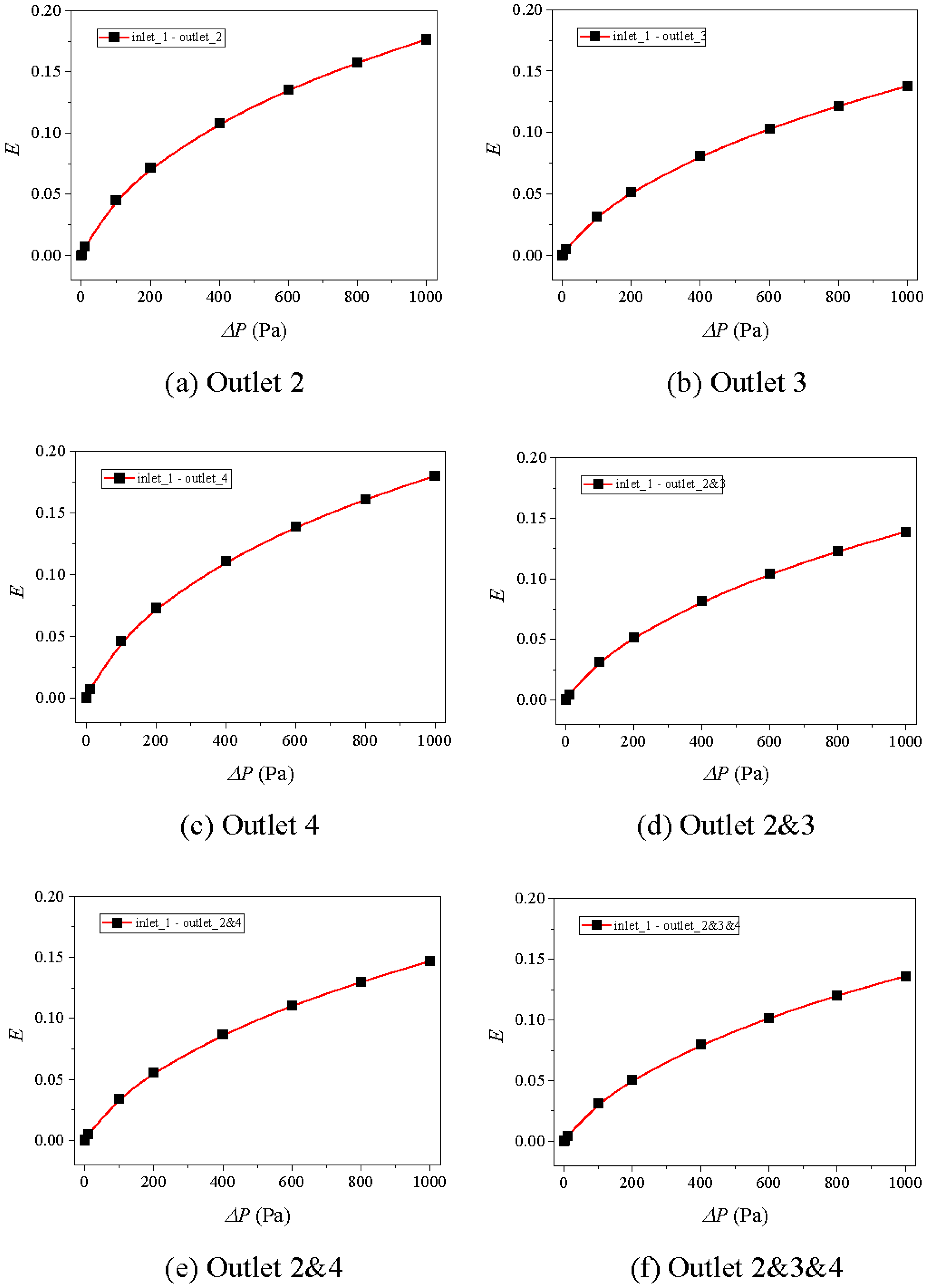
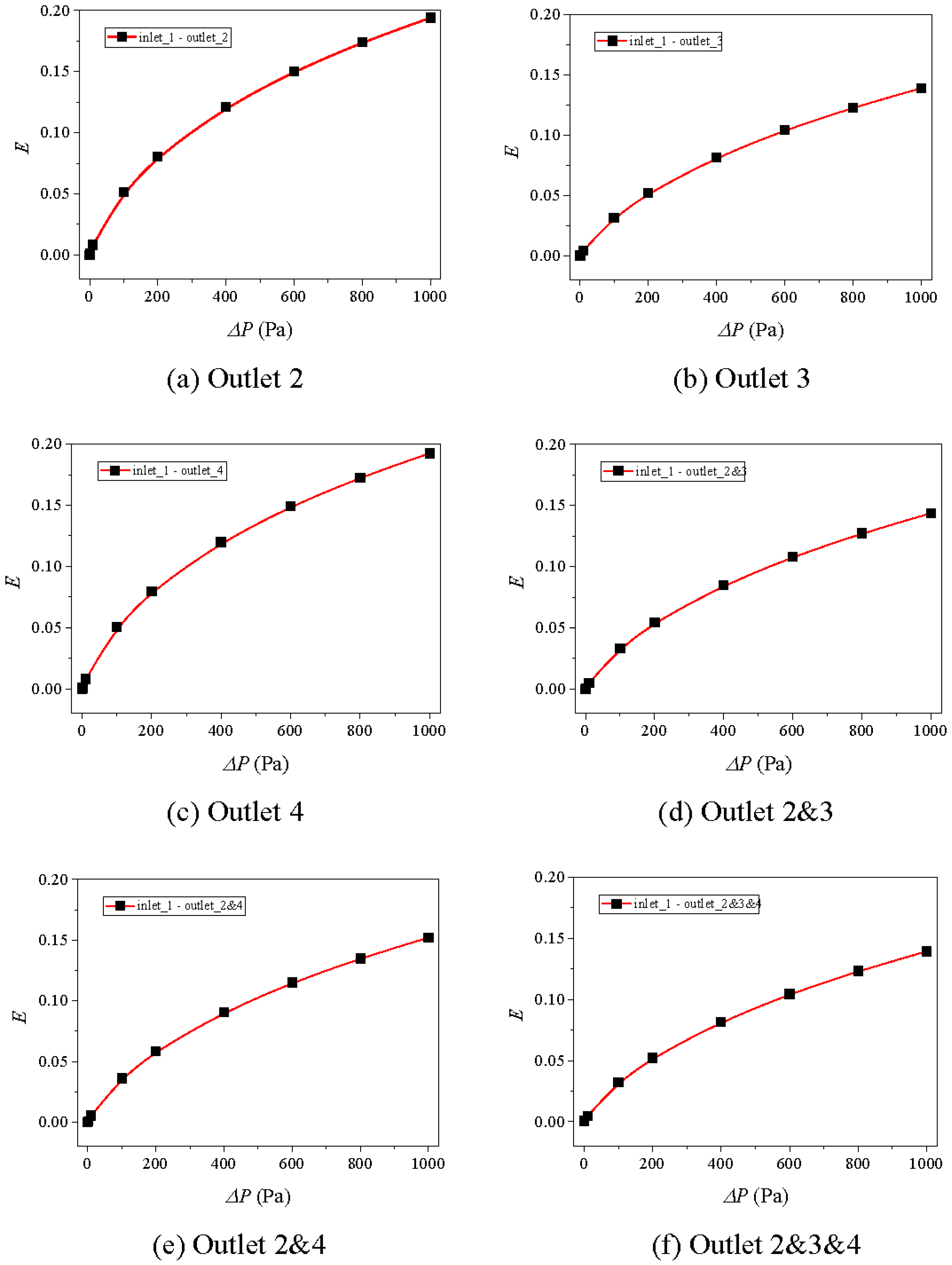
The nonlinear factor E defined in Equation (3) is adopted to quantify the nonlinearity of fluid flow in rock fractures [51,60]. Figure 10, Figure 11 and Figure 12 exhibit the variations of E versus ΔP hat ranges from 0 to 1000 Pa. The results show that with the increment ΔP, E increases first fast and then gently, and finally approaches constant values. With increasing the number of outlets, for examples from 1 outlet (i.e., outlet 2 in Figure 11a) to 2 outlets (i.e., outlet 2 and 4 in Figure 11e), or to 3 outlets (i.e., outlet 2 and 3 and 4 in Figure 11f), for the same ΔP, E decreases. This is because a greater number of outlets indicate the larger flow volume, and the larger fracture aperture (or flow volume) corresponds to a weaker nonlinearity of fluid flow that is represented by a smaller E [55]. When increasing apertures of segments 2 and 4 from 3 mm to 5 mm (from Figure 10 to Figure 11), the E~ΔP curves move downwards significantly. However, when increasing apertures of segments 2 and 4 from 5 mm to 7 mm (from Figure 11 to Figure 12), the Q~ΔP curve variation is negligibly small. This indicates that the E~ΔP curves are more sensitive to fractures that have smaller apertures, which have the same variation trend with those of Q~ΔP curves as illustrated in Section 5.2.1.
5.2.3. Effect of Fracture Aperture on ΔPc
Figure 13 depicts the relationships between the critical hydraulic difference (ΔPc) that corresponds to E = 0.1 and aperture of segments 2 and 4. For the six cases considered, with the increment of aperture of segments 2 and 4 from 3 mm to 5 mm, the average ΔPc increases significantly from 38.84 Pa to 489.38 Pa. However, with continuously increasing aperture of segments 2 and 4 from 5 mm to 7 mm, the average ΔPc changes slightly, or even decreases to some extent. This indicates that ΔPc is more sensitive to a smaller aperture of segments 2 and 4. Before selecting the governing equation for modeling fluid flow in rock fractures, the applied pressure difference should be compared with ΔPc. When the applied pressure difference is less than ΔPc, the cubic law that can be simply solved should be selected. When the applied pressure difference is larger than ΔPc, the Navier-Stokes equations or the Forchheimer’s law should be adopted to solve the nonlinear flow through rock fractures/fracture networks.
5.2.4. Effect of Fracture Aperture on e/E0~ΔP Curves
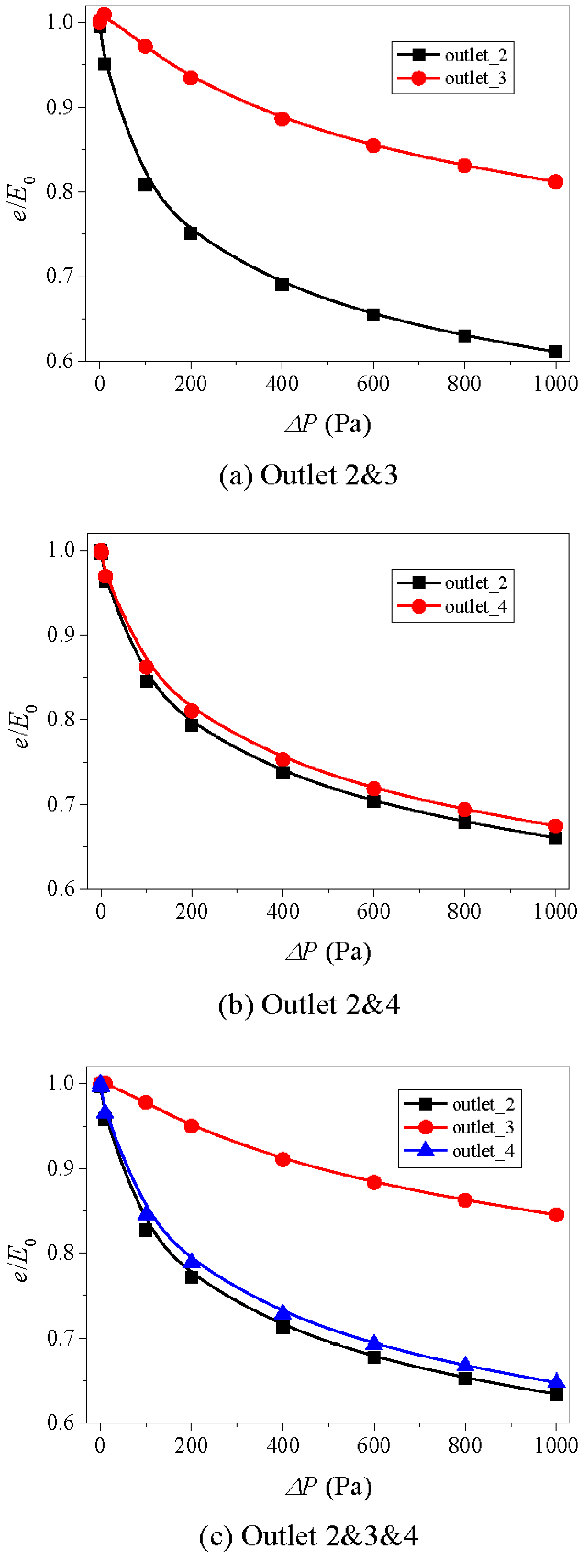
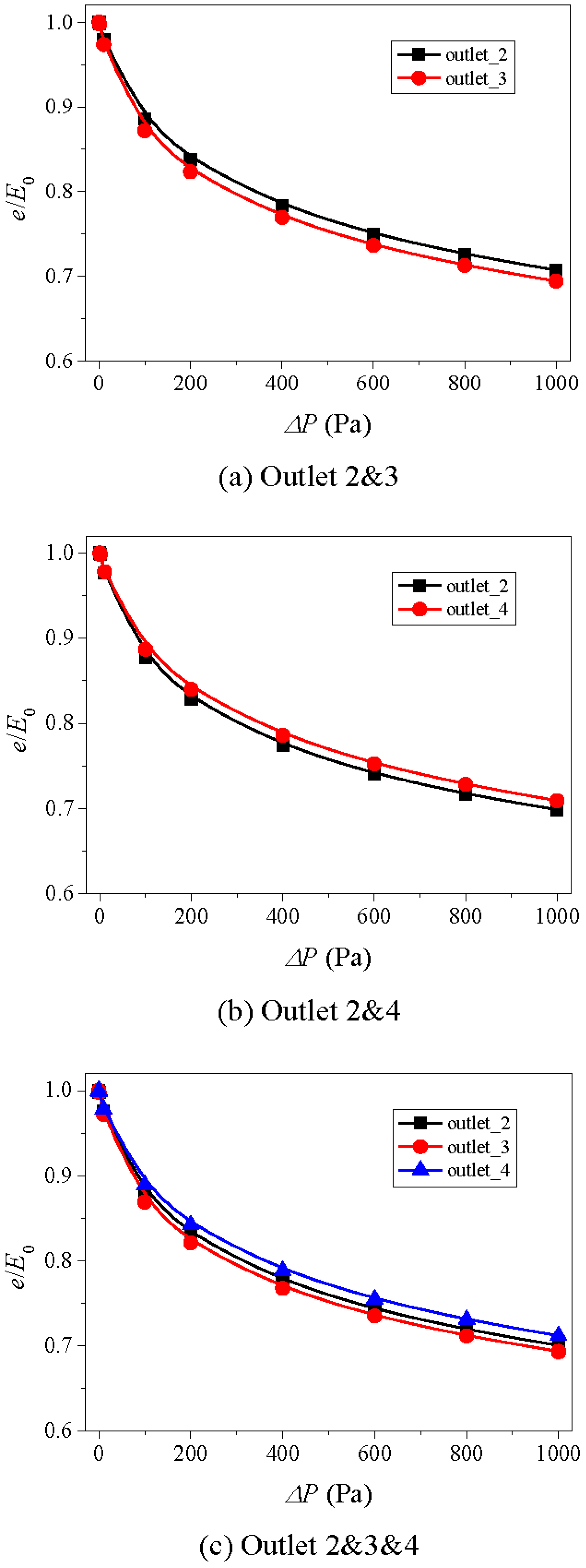
In Equation (2), e is the hydraulic aperture, and in Table 1, E0 is the mechanical aperture. Generally, to quantify the effect of parameters such as fracture surface roughness, Reynolds number and contact on the hydraulic properties of rock fractures, the ratio of hydraulic aperture to mechanical aperture is utilized [61,62,63]. Therefore, the influence of aperture of segments 2 and 4 on the variations of e/E0 was analyzed in this section and the results are presented in Figure 14, Figure 15 and Figure 16. For each case, with increasing ΔP when ΔP is large, the fluid flow enters the nonlinear flow regime and energy losses due to the formation of eddies. As a result, the value of ΔQ/ΔP decreases and then the e that is back-calculated according to Equation (2) decreases. Thus, e/E0 decreases, and the decreasing rate decreases as ΔP increases. In Figure 14, since the apertures of the two crossed fractures are both 3 mm, the variations of e/E0 versus ΔP have the same trends and orders of magnitude. When increasing the aperture of segments 2 and 4 to 5 mm, the results show that the e/E0 of segment 2, which is represented by outlet 2 in Figure 15a, decreases more significantly than that of segment 3, and the decreasing rate of e/E0 of segment 2 is smaller than that of segment 3. Since the apertures of segments 2 and 4 are the same, that is 5 mm, the variations of e/E0 of segments 2 and 4 are close to each other as shown in Figure 15b. Figure 15c shows the same results as that in Figure 15, in which the variations of e/E0 of segment that has a larger aperture (i.e., segments 2 and 4 that have an aperture of 5 mm) are more robust than one with a smaller aperture (i.e., segment 3 that has an aperture of 3 mm). With continuously increasing the aperture of segments 2 and 4 to 7 mm, the variations of e/E0 as shown in Figure 16 are close to those shown in Figure 15. The difference is that the decreasing degree of e/E0 of a segment that has a larger aperture is more significant. Therefore, even though increasing aperture of segments 2 and 4 from 5 mm to 7 had a negligibly small effect on the ΔPc, its influence on e/E0 cannot be negligible and should be considered.
6. Conclusions
In the present study, fluid flow tests on three crossed fracture models were carried out, and the geometries of the fractures were accurately obtained using visualization techniques. Three numerical models that corresponded to the three experimental models were established, and fluid flow was modelled by solving the Navier-Stokes equations. Finally, another three numerical models were established to perform parametric studies to quantify the onset of nonlinear flow and to systematically investigate the variations of the ratio of hydraulic aperture to mechanical aperture.
The results show that the numerical simulation results agree well with those of the fluid flow tests, indicating that the visualization techniques and the numerical simulation code are reliable. With the increment of flow rate, the pressure difference first increases linearly and then nonlinearly, which can be best fitted using Forchheimer’s law. The two coefficients in Forchheimer’s law decrease with the increasing number of outlets. With the increment of pressure difference, the nonlinear factor first increases significantly and then gently, and finally approaches constant values. The nonlinear factor—pressure difference curves are more sensitive to fractures that have smaller apertures. With the increment of pressure difference, the ratio of hydraulic aperture to mechanical aperture decrease and the decreasing rate decreases. The ratio of hydraulic aperture to mechanical aperture decreases more significantly for a fracture that has a larger aperture.
Note that the present study assumes that the rock matrix is impermeable. However, in practical engineering, the rock matrix is a porous media and fluid flows through it. Therefore, the interaction between a fracture and a rock matrix may play a significant role in the exchange of fluid. The present study adopts an aperture of 3–7 mm for rock fractures, which is much larger than that of fractures deep underground. Further, the influence of fracture length ratio and combinations of different inlets and outlets (i.e., two inlets and one outlet, two inlets and two outlets) on the nonlinear flow regimes are not taken into account. All of these should be the focus of our future works.
7. Data Availability
All the data used in the present study are available by connecting the corresponding author and/or the first author. Their emails are [email protected] (Yujing Jiang) and [email protected] (Richeng Liu), respectively.
Author Contributions
R.L. and Y.J. conceived and designed the experiments; R.L. performed the experiments; R.L. and H.J. analyzed the data; Y.J. and L.Y. contributed reagents/materials/analysis tools; R.L. wrote the paper.
Funding
This research received no external funding.
Acknowledgments
This study has been partially funded by National Natural Science Foundation of China (Grant Nos. 51734009, 51709260, 51579239), Japan Society for the Promotion of Science (JSPS) (Grant No. P17382), and Natural Science Foundation of Jiangsu Province, China (Grant No. BK20170276). These supports are gratefully acknowledged.
Conflicts of Interest
The authors declare no conflicts of interest.
References
- Juanes, R.; Spiteri, E.J.; Orr, F.M.; Blunt, M.J. Impact of relative permeability hysteresis on geological CO2 storage. Water Resour. Res. 2006, 42. [Google Scholar] [CrossRef]
- Oya, S.; Aifaa, M.; Ohmura, R. Formation, growth and sintering of CO2 hydrate crystals in liquid water with continuous CO2 supply: Implication for subsurface CO2 sequestration. Int. J. Greenh. Gas Control 2017, 63, 386–391. [Google Scholar] [CrossRef]
- Rubinstein, J.L.; Mahani, A.B. Myths and facts on wastewater injection, hydraulic fracturing, enhanced oil recovery, and induced seismicity. Seismol. Res. Lett. 2015, 86, 1060–1067. [Google Scholar] [CrossRef]
- Cai, J.; Wei, W.; Hu, X.; Liu, R.; Wang, J. Fractal characterization of dynamic fracture network extension in porous media. Fractals 2017, 25. [Google Scholar] [CrossRef]
- Juanes, R.; Tchelepi, H.A. Special issue on multiscale methods for flow and transport in heterogeneous porous media. Comput. Geosci. 2008, 12, 255–256. [Google Scholar] [CrossRef]
- Zhao, C.; Hobbs, B.E.; Ord, A. Chemical dissolution-front instability associated with water-rock reactions in groundwater hydrology: Analyses of porosity-permeability relationship effects. J. Hydrol. 2016, 540, 1078–1087. [Google Scholar] [CrossRef]
- Wei, W.; Xia, Y. Geometrical, fractal and hydraulic properties of fractured reservoirs: A. mini-review. Adv. Geo-Energy Res. 2017, 1, 31–38. [Google Scholar] [CrossRef]
- Wang, C.; Liu, J.; Feng, J.; Wei, M.; Wang, C.; Jiang, Y. Effects of gas diffusion from fractures to coal matrix on the evolution of coal strains: Experimental observations. Int. J. Coal Geol. 2016, 162, 74–84. [Google Scholar] [CrossRef]
- Wang, C.; Zhai, P.; Chen, Z.; Liu, J.; Wang, L.; Xie, J. Experimental study of coal matrix-cleat interaction under constant volume boundary condition. Int. J. Coal Geol. 2017, 181, 124–132. [Google Scholar] [CrossRef]
- Baghbanan, A.; Jing, L. Hydraulic properties of fractured rock masses with correlated fracture length and aperture. Int. J. Rock Mech. Min. Sci. 2007, 44, 704–719. [Google Scholar] [CrossRef]
- Jafari, A.; Babadagli, T. Estimation of equivalent fracture network permeability using fractal and statistical network properties. J. Pet. Sci. Eng. 2012, 92, 110–123. [Google Scholar] [CrossRef]
- Zhou, J.Q.; Wang, M.; Wang, L.C.; Chen, Y.F.; Zhou, C.B. Emergence of Nonlinear Laminar Flow in Fractures During Shear. Rock Mech. Rock Eng. 2018, 1–9. [Google Scholar] [CrossRef]
- Zhou, J.Q.; Hu, S.H.; Fang, S.; Chen, Y.; Zhou, C. Nonlinear flow behavior at low Reynolds numbers through rough-walled fractures subjected to normal compressive loading. Int. J. Rock Mech. Min. Sci. 2015, 80, 202–218. [Google Scholar] [CrossRef]
- Long, J.C.S.; Remer, J.S.; Wilson, C.R.; Witherspoon, P.A. Porous media equivalents for networks of discontinuous fractures. Water Resour. Res. 1982, 18, 645–658. [Google Scholar] [CrossRef] [Green Version]
- Tsang, C.F. Is current hydrogeologic research addressing long-term predictions? Groundwater 2005, 43, 296–300. [Google Scholar] [CrossRef] [PubMed] [Green Version]
- Hartley, L.; Roberts, D. Summary of Discrete Fracture Network Modelling as Applied to Hydrogeology of the Forsmark and Laxemar Sites; Report, R.-12-04; Swedish Nuclear Fuel and Waste Management Co.: Stockholm, Sweden, 2012. [Google Scholar]
- Min, K.B.; Rutqvist, J.; Tsang, C.F.; Jing, L. Stress-dependent permeability of fractured rock masses: A numerical study. Int. J. Rock Mech. Min. Sci. 2004, 41, 1191–1210. [Google Scholar] [CrossRef]
- Lei, Q.; Latham, J.P.; Tsang, C.F.; Xiang, J.; Lang, P. A new approach to upscaling fracture network models while preserving geostatistical and geomechanical characteristics. J. Geophys. Res. Solid Earth 2015, 120, 4784–4807. [Google Scholar] [CrossRef] [Green Version]
- Zhang, Q.; Zhang, C.; Jiang, B.; Li, N.; Wang, Y. Elastoplastic coupling solution of circular openings in strain-softening rock mass considering pressure-dependent effect. Int. J. Geomech. 2018, 18. [Google Scholar] [CrossRef]
- Liu, R.; Li, B.; Jiang, Y.; Yu, L. A numerical approach for assessing effects of shear on equivalent permeability and nonlinear flow characteristics of 2-D. fracture networks. Adv. Water Resour. 2018, 111, 289–300. [Google Scholar] [CrossRef]
- Kosakowski, G.; Berkowitz, B. Flow pattern variability in natural fracture intersections. Geophys. Res. Lett. 1999, 26, 1765–1768. [Google Scholar] [CrossRef] [Green Version]
- Chen, Y.F.; Hu, S.H.; Hu, R.; Zhou, C.B. Estimating hydraulic conductivity of fractured rocks from high-pressure packer tests with an Izbash’s law-based empirical model. Water Resour. Res. 2015, 51, 2096–2118. [Google Scholar] [CrossRef]
- Brown, S.R.; Scholz, C.H. Broad bandwidth study of the topography of natural rock surfaces. J. Geophys. Res. Solid Earth 1985, 90, 12575–12582. [Google Scholar] [CrossRef]
- Javadi, M.; Sharifzadeh, M.; Shahriar, K. A new geometrical model for non-linear fluid flow through rough fractures. J. Hydrol. 2010, 389, 18–30. [Google Scholar] [CrossRef]
- Zimmerman, R.W.; Bodvarsson, G.S. Hydraulic conductivity of rock fractures. Transp. Porous Media 1996, 23, 1–30. [Google Scholar] [CrossRef]
- Li, B.; Jiang, Y.; Koyama, T.; Jing, L.; Tanabashi, Y. Experimental study of the hydro-mechanical behavior of rock joints using a parallel-plate model containing contact areas and artificial fractures. Int. J. Rock Mech. Min. Sci. 2008, 45, 362–375. [Google Scholar] [CrossRef] [Green Version]
- Koyama, T.; Neretnieks, I.; Jing, L. A numerical study on differences in using Navier–Stokes and Reynolds equations for modeling the fluid flow and particle transport in single rock fractures with shear. Int. J. Rock Mech. Min. Sci. 2008, 45, 1082–1101. [Google Scholar] [CrossRef] [Green Version]
- Javadi, M.; Sharifzadeh, M.; Shahriar, K.; Mitani, Y. Critical Reynolds number for nonlinear flow through rough-walled fractures: The role of shear processes. Water Resour. Res. 2014, 50, 1789–1804. [Google Scholar] [CrossRef] [Green Version]
- Rong, G.; Hou, D.; Yang, J.; Cheng, L.; Zhou, C. Experimental study of flow characteristics in non-mated rock fractures considering 3D definition of fracture surfaces. Eng. Geol. 2017, 220, 152–163. [Google Scholar] [CrossRef]
- Yin, Q.; Ma, G.; Jing, H.; Su, H.; Wang, Y.; Liu, R. Hydraulic properties of 3D rough-walled fractures during shearing: An experimental study. J. Hydrol. 2017, 555, 169–184. [Google Scholar] [CrossRef]
- Liu, R.; Jiang, Y.; Li, B. Effects of intersection and dead-end of fractures on nonlinear flow and particle transport in rock fracture networks. Geosci. J. 2016, 20, 415–426. [Google Scholar] [CrossRef]
- Li, B.; Liu, R.; Jiang, Y. Influences of hydraulic gradient, surface roughness, intersecting angle, and scale effect on nonlinear flow behavior at single fracture intersections. J. Hydrol. 2016, 538, 440–453. [Google Scholar] [CrossRef]
- Wu, Z.; Fan, L.; Zhao, S. Effects of hydraulic gradient, intersecting angle, aperture and fracture length on the nonlinearity of fluid flow in smooth intersecting fractures: An experimental investigation. Geofluids 2018, 2018, 9352608. [Google Scholar] [CrossRef]
- Bear, J. Dynamics of Fluids in Porous Media; Elsevier: New York, NY, USA; London, UK; Amsterdam, The Netherlands, 1972. [Google Scholar]
- De Dreuzy, J.R.; Davy, P.; Bour, O. Hydraulic properties of two-dimensional random fracture networks following a power law length distribution: 2. Permeability of networks based on lognormal distribution of apertures. Water Resour. Res. 2001, 37, 2079–2095. [Google Scholar] [CrossRef] [Green Version]
- De Dreuzy, J.R.; Davy, P.; Bour, O. Hydraulic properties of two-dimensional random fracture networks following power law distributions of length and aperture. Water Resour. Res. 2002, 38, 12-1–12-9. [Google Scholar] [CrossRef]
- Dverstorp, B.; Andersson, J. Application of the discrete fracture network concept with field data: Possibilities of model calibration and validation. Water Resour. Res. 1989, 25, 540–550. [Google Scholar] [CrossRef]
- Cacas, M.C.; Ledoux, E.; Marsily, G.; Tillie, B.; Barbreau, A.; Durand, E.; Feuga, B.; Peaudecerf, P. Modeling fracture flow with a stochastic discrete fracture network: Calibration and validation: 1. The flow model. Water Resour. Res. 1990, 26, 479–489. [Google Scholar] [CrossRef]
- Li, J.H.; Zhang, L.M. Geometric parameters and REV of a crack network in soil. Comput. Geotech. 2010, 37, 466–475. [Google Scholar] [CrossRef]
- Hatton, C.G.; Main, I.G.; Meredith, P.G. Non-universal of fracture length and opening displacement. Nature 1994, 367, 160–162. [Google Scholar] [CrossRef]
- Renshaw, C.E.; Park, J.C. Effect of mechanical interactions on the scaling of fracture length and aperture. Nature 1997, 386, 482–484. [Google Scholar] [CrossRef]
- Bonnet, E.; Bour, O.; Odling, N.E.; Davy, P.; Main, I.; Cowie, P.; Berkowitz, B. Scaling of fracture systems in geological media. Rev. Geophys. 2001, 39, 347–383. [Google Scholar] [CrossRef] [Green Version]
- Zimmerman, R.; Main, I. Hydromechanical behavior of fractured rocks. Int. Geophys. Serv. 2004, 89, 363–422. [Google Scholar]
- Schultz, R.A.; Soliva, R.; Fossen, H.; Okubo, C.H. Dependence of displacement–length scaling relations for fractures and deformation bands on the volumetric changes across them. J. Struct. Geol. 2008, 30, 1405–1411. [Google Scholar] [CrossRef]
- Klimczak, C.; Schultz, R.A.; Parashar, R.; Reeves, D.M. Cubic law with aperture-length correlation: Implications for network scale fluid flow. Hydrogeol. J. 2010, 18, 851–862. [Google Scholar] [CrossRef]
- Liu, R.; Li, B.; Jiang, Y.; Huang, N. Review: Mathematical expressions for estimating equivalent permeability of rock fracture networks. Hydrogeol. J. 2016, 24, 1623–1649. [Google Scholar] [CrossRef]
- Neuville, A.; Flekkøy, E.G.; Toussaint, R. Influence of asperities on fluid and thermal flow in a fracture: A coupled Lattice Boltzmann study. J. Geophys. Res. Solid Earth 2013, 118, 3394–3407. [Google Scholar] [CrossRef] [Green Version]
- Xiong, X.; Li, B.; Jiang, Y.; Koyama, T.; Zhang, C. Experimental and numerical study of the geometrical and hydraulic characteristics of a single rock fracture during shear. Int. J. Rock Mech. Min. Sci. 2011, 48, 1292–1302. [Google Scholar] [CrossRef]
- Min, K.B.; Jing, L. Numerical determination of the equivalent elastic compliance tensor for fractured rock masses using the distinct element method. Int. J. Rock Mech. Min. Sci. 2003, 40, 795–816. [Google Scholar] [CrossRef]
- Wang, Z.; Li, W.; Bi, L.; Qiao, L.; Liu, R.; Liu, J. Estimation of the REV Size and Equivalent Permeability Coefficient of Fractured Rock Masses with an Emphasis on Comparing the Radial and Unidirectional Flow Configurations. Rock Mech. Rock Eng. 2018, 51, 1457–1471. [Google Scholar] [CrossRef]
- Zimmerman, R.W.; Al-Yaarubi, A.; Painl, C.C.; Grattoni, C.A. Non-linear regimes of fluid flow in rock fractures. Int. J. Rock Mech. Min. Sci. 2004, 41, 163–169. [Google Scholar] [CrossRef]
- Qian, J.; Zhan, H.; Chen, Z.; Ye, H. Experimental study of solute transport under non-Darcian flow in a single fracture. J. Hydrol. 2011, 399, 246–254. [Google Scholar] [CrossRef]
- Adler, P.M.; Malevich, A.E.; Mityushev, V.V. Nonlinear correction to Darcy’s law for channels with wavy walls. Acta Mech. 2013, 224, 1823–1848. [Google Scholar] [CrossRef]
- Zeng, Z.; Grigg, R. A criterion for non-Darcy flow in porous media. Transp. Porous Media 2006, 63, 57–69. [Google Scholar] [CrossRef]
- Liu, R.; Li, B.; Jiang, Y. Critical hydraulic gradient for nonlinear flow through rock fracture networks: The roles of aperture, surface roughness, and number of intersections. Adv. Water Resour. 2016, 88, 53–65. [Google Scholar] [CrossRef]
- Wang, M.; Chen, Y.F.; Ma, G.W.; Zhou, J.Q. Influence of surface roughness on nonlinear flow behaviors in 3D self-affine rough fractures: Lattice Boltzmann simulations. Adv. Water Resour. 2016, 96, 373–388. [Google Scholar] [CrossRef]
- Szymczak, P.; Ladd, A.J.C. Wormhole formation in dissolving fractures. J. Geophys. Res. Solid Earth 2009, 114. [Google Scholar] [CrossRef] [Green Version]
- Myers, N.O. Characterization of surface roughness. Wear 1962, 5, 182–189. [Google Scholar] [CrossRef]
- Tse, R.; Cruden, D.M. Estimating joint roughness coefficients. Int. J. Rock Mech. Min. Sci. 1979, 16, 303–307. [Google Scholar] [CrossRef]
- Yu, L.; Liu, R.; Jiang, Y. A review of critical conditions for the onset of nonlinear fluid flow in rock fractures. Geofluids 2017, 2017, 2176932. [Google Scholar] [CrossRef]
- Barton, N.; Bandis, S.; Bakhtar, K. Strength, deformation and conductivity coupling of rock joints. Int. J. Rock Mech. Min. Sci. 1985, 22, 121–140. [Google Scholar] [CrossRef]
- Olsson, R.; Barton, N. An improved model for hydromechanical coupling during shearing of rock joints. Int. J. Rock Mech. Min. Sci. 2001, 38, 317–329. [Google Scholar] [CrossRef]
- Rasouli, V.; Hosseinian, A. Correlations developed for estimation of hydraulic parameters of rough fractures through the simulation of JRC flow channels. Rock Mech. Rock Eng. 2011, 44, 447–461. [Google Scholar] [CrossRef]
Figure 1.
A crossed fracture model with one inlet and three outlets.

Figure 2.
Experimental system of fluid flow test.

Figure 3.
Enlarged views of fracture intersection of three numerical models.
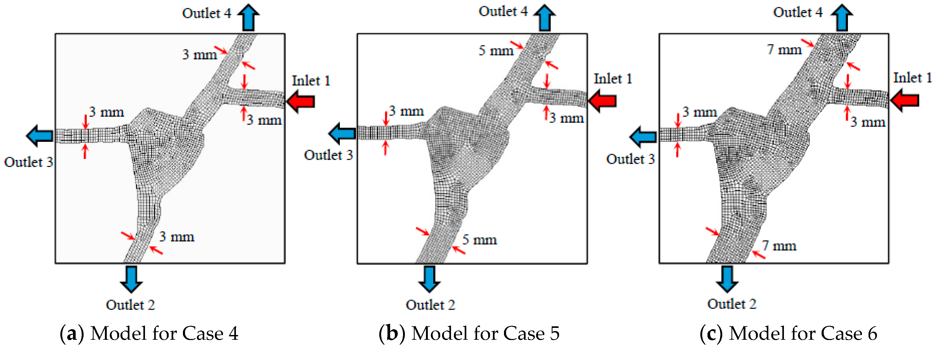
Figure 4.
Comparisons of Q~P curves between simulation and test results for Case 1 with different combinations of outlets: (a) outlet 2, (b) outlet 3, (c) outlet 4, (d) outlet 2 and 3, (e) outlet 2 and 4, (f) outlet 2 and 3 and 4.
Figure 4.
Comparisons of Q~P curves between simulation and test results for Case 1 with different combinations of outlets: (a) outlet 2, (b) outlet 3, (c) outlet 4, (d) outlet 2 and 3, (e) outlet 2 and 4, (f) outlet 2 and 3 and 4.


Figure 5.
Comparisons of Q~P curves between simulation and test results for Case 2 with different combinations of outlets: (a) outlet 2, (b) outlet 3, (c) outlet 4, (d) outlet 2 and 3, (e) outlet 2 and 4, (f) outlet 2 and 3 and 4.
Figure 5.
Comparisons of Q~P curves between simulation and test results for Case 2 with different combinations of outlets: (a) outlet 2, (b) outlet 3, (c) outlet 4, (d) outlet 2 and 3, (e) outlet 2 and 4, (f) outlet 2 and 3 and 4.


Figure 6.
Comparisons of Q~P curves between simulation and test results for Case 3 with different combinations of outlets: (a) outlet 2, (b) outlet 3, (c) outlet 4, (d) outlet 2 and 3, (e) outlet 2 and 4, (f) outlet 2 and 3 and 4.
Figure 6.
Comparisons of Q~P curves between simulation and test results for Case 3 with different combinations of outlets: (a) outlet 2, (b) outlet 3, (c) outlet 4, (d) outlet 2 and 3, (e) outlet 2 and 4, (f) outlet 2 and 3 and 4.
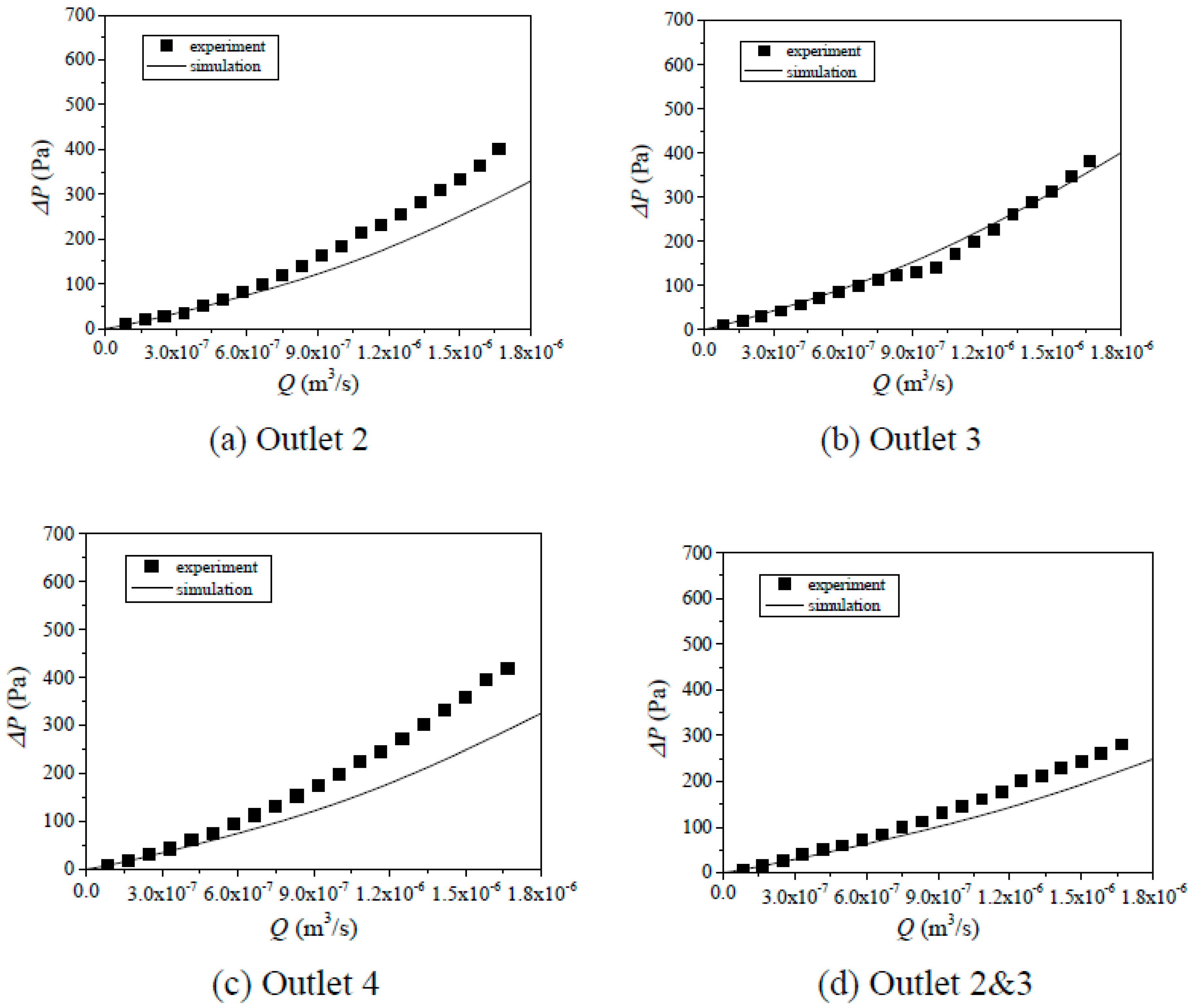

Figure 7.
Variations of Q~P curves for Case 4 with different combinations of outlets: (a) outlet 2, (b) outlet 3, (c) outlet 4, (d) outlet 2 and 3, (e) outlet 2 and 4, (f) outlet 2 and 3 and 4.
Figure 7.
Variations of Q~P curves for Case 4 with different combinations of outlets: (a) outlet 2, (b) outlet 3, (c) outlet 4, (d) outlet 2 and 3, (e) outlet 2 and 4, (f) outlet 2 and 3 and 4.

Figure 8.
Variations of Q~P curves for Case 5 with different combinations of outlets: (a) outlet 2, (b) outlet 3, (c) outlet 4, (d) outlet 2 and 3, (e) outlet 2 and 4, (f) outlet 2 and 3 and 4.
Figure 8.
Variations of Q~P curves for Case 5 with different combinations of outlets: (a) outlet 2, (b) outlet 3, (c) outlet 4, (d) outlet 2 and 3, (e) outlet 2 and 4, (f) outlet 2 and 3 and 4.

Figure 9.
Variations of Q~P curves for Case 6 with different combinations of outlets: (a) outlet 2, (b) outlet 3, (c) outlet 4, (d) outlet 2 and 3, (e) outlet 2 and 4, (f) outlet 2 and 3 and 4.
Figure 9.
Variations of Q~P curves for Case 6 with different combinations of outlets: (a) outlet 2, (b) outlet 3, (c) outlet 4, (d) outlet 2 and 3, (e) outlet 2 and 4, (f) outlet 2 and 3 and 4.

Figure 10.
Variations of E~P curves for Case 4 with different combinations of outlets: (a) outlet 2, (b) outlet 3, (c) outlet 4, (d) outlet 2 and 3, (e) outlet 2 and 4, (f) outlet 2 and 3 and 4.
Figure 10.
Variations of E~P curves for Case 4 with different combinations of outlets: (a) outlet 2, (b) outlet 3, (c) outlet 4, (d) outlet 2 and 3, (e) outlet 2 and 4, (f) outlet 2 and 3 and 4.

Figure 11.
Variations of E~P curves for Case 5 with different combinations of outlets: (a) outlet 2, (b) outlet 3, (c) outlet 4, (d) outlet 2 and 3, (e) outlet 2 and 4, (f) outlet 2 and 3 and 4.
Figure 11.
Variations of E~P curves for Case 5 with different combinations of outlets: (a) outlet 2, (b) outlet 3, (c) outlet 4, (d) outlet 2 and 3, (e) outlet 2 and 4, (f) outlet 2 and 3 and 4.

Figure 12.
Variations of E~P curves for Case 6 with different combinations of outlets: (a) outlet 2, (b) outlet 3, (c) outlet 4, (d) outlet 2 and 3, (e) outlet 2 and 4, (f) outlet 2 and 3 and 4.
Figure 12.
Variations of E~P curves for Case 6 with different combinations of outlets: (a) outlet 2, (b) outlet 3, (c) outlet 4, (d) outlet 2 and 3, (e) outlet 2 and 4, (f) outlet 2 and 3 and 4.

Figure 13.
Relationships between ΔPc and aperture of segments 2 and 4.
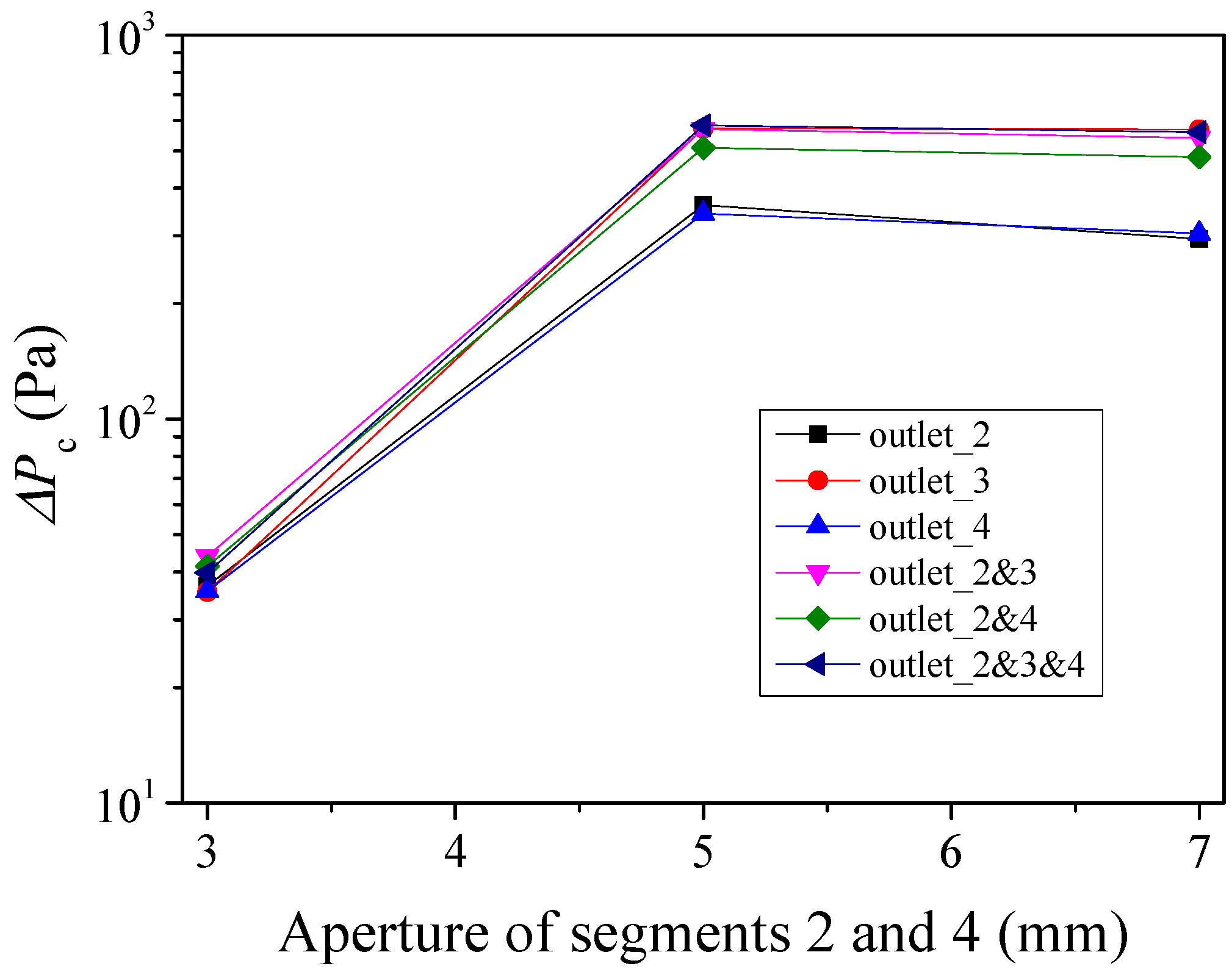
Figure 14.
Variations of e/E0~P curves for Case 4 with different combinations of outlets: (a) outlet 2 and 3, (b) outlet 2 and 4, (c) outlet 2 and 3 and 4.
Figure 14.
Variations of e/E0~P curves for Case 4 with different combinations of outlets: (a) outlet 2 and 3, (b) outlet 2 and 4, (c) outlet 2 and 3 and 4.

Figure 15.
Variations of e/E0~P curves for Case 5 with different combinations of outlets: (a) outlet 2 and 3, (b) outlet 2 and 4, (c) outlet 2 and 3 and 4.
Figure 15.
Variations of e/E0~P curves for Case 5 with different combinations of outlets: (a) outlet 2 and 3, (b) outlet 2 and 4, (c) outlet 2 and 3 and 4.

Figure 16.
Variations of e/E0~P curves for Case 6 with different combinations of outlets: (a) outlet 2 and 3, (b) outlet 2 and 4, (c) outlet 2 and 3 and 4.
Figure 16.
Variations of e/E0~P curves for Case 6 with different combinations of outlets: (a) outlet 2 and 3, (b) outlet 2 and 4, (c) outlet 2 and 3 and 4.

Table 1.
Parameters of fracture segments for different cases.
| Case No. | Segment No. | Lt (mm) | E0 (mm) | Z2 | Number of Hexahedral Cells |
|---|---|---|---|---|---|
| 1 | 1 | 220.27 | 2.70 | 0.42 | 212,320 |
| 2 | 241.97 | 2.63 | 0.25 | ||
| 3 | 207.33 | 2.48 | 0.18 | ||
| 4 | 240.53 | 2.06 | 0.15 | ||
| 2 | 1 | 220.27 | 2.81 | 0.42 | 243,830 |
| 2 | 241.97 | 3.61 | 0.25 | ||
| 3 | 207.33 | 2.52 | 0.18 | ||
| 4 | 240.53 | 3.88 | 0.15 | ||
| 3 | 1 | 220.27 | 2.89 | 0.42 | 305,070 |
| 2 | 241.97 | 6.45 | 0.25 | ||
| 3 | 207.33 | 3.2 | 0.18 | ||
| 4 | 240.53 | 6.09 | 0.15 | ||
| 4 | 1 | 220.27 | 3 | 0.42 | 229,140 |
| 2 | 241.97 | 3 | 0.25 | ||
| 3 | 207.33 | 3 | 0.18 | ||
| 4 | 240.53 | 3 | 0.15 | ||
| 5 | 1 | 220.27 | 3 | 0.42 | 275,720 |
| 2 | 241.97 | 5 | 0.25 | ||
| 3 | 207.33 | 3 | 0.18 | ||
| 4 | 240.53 | 5 | 0.15 | ||
| 6 | 1 | 220.27 | 3 | 0.42 | 323,060 |
| 2 | 241.97 | 7 | 0.25 | ||
| 3 | 207.33 | 3 | 0.18 | ||
| 4 | 240.53 | 7 | 0.15 |
© 2018 by the authors. Licensee MDPI, Basel, Switzerland. This article is an open access article distributed under the terms and conditions of the Creative Commons Attribution (CC BY) license (http://creativecommons.org/licenses/by/4.0/).
Share and Cite
MDPI and ACS Style
Liu, R.; Jiang, Y.; Jing, H.; Yu, L. Nonlinear Flow Characteristics of a System of Two Intersecting Fractures with Different Apertures. Processes 2018, 6, 94. https://doi.org/10.3390/pr6070094
AMA Style
Liu R, Jiang Y, Jing H, Yu L. Nonlinear Flow Characteristics of a System of Two Intersecting Fractures with Different Apertures. Processes. 2018; 6(7):94. https://doi.org/10.3390/pr6070094
Chicago/Turabian StyleLiu, Richeng, Yujing Jiang, Hongwen Jing, and Liyuan Yu. 2018. "Nonlinear Flow Characteristics of a System of Two Intersecting Fractures with Different Apertures" Processes 6, no. 7: 94. https://doi.org/10.3390/pr6070094
Note that from the first issue of 2016, this journal uses article numbers instead of page numbers. See further details here.