The Fracturing Behavior of Tight Glutenites Subjected to Hydraulic Pressure
by
 ,
,
Zhichao Li
1, 
Lianchong Li
2,*,
Zilin Zhang
3,
Ming Li
3,
Liaoyuan Zhang
3,
Bo Huang
3 and
Chun’an Tang
1 1
State Key Laboratory of Coastal and Offshore Engineering, Dalian University of Technology, Dalian 116024, China
2
School of Resources and Civil Engineering, Northeastern University, Shenyang 110819, China
3
Shengli Oilfield Branch Company, SINOPEC, Dongying 257000, China
*
Author to whom correspondence should be addressed.
Processes 2018, 6(7), 96; https://doi.org/10.3390/pr6070096
Submission received: 5 July 2018
/
Revised: 19 July 2018
/
Accepted: 19 July 2018
/
Published: 20 July 2018
(This article belongs to the Special Issue Fluid Flow in Fractured Porous Media)
Abstract
:Tight glutenites are typically composed of heterogeneous sandstone and gravel. Due to low or ultra-low permeability, it is difficult to achieve commercial production in tight glutenites without hydraulic fracturing. Efficient exploitation requires an in-depth understanding of the fracturing behavior of these reservoirs. This paper provides a numerical method that integrates the digital image processing (DIP) technique into a numerical code rock failure process analysis (RFPA). This method could consider the glutenite heterogeneities, including intrarock and interrock heterogeneities, and the practicability is verified through two numerical tests. Two-dimensional (2D) simulations show hydraulic fractures (HFs) can penetrate or deflect to propagate along the gravels, depending on the magnitude of stress anisotropy and gravel strength. Three-dimensional (3D) simulations with the consideration of gravel distribution orientation, gravel size and axial ratio show HFs could propagate past the gravel with no deflection, forming a bypass fracture that is not easy to observe in common laboratory experiments. HFs could also deflect to propagate along the gravels. The impacts of the gravel distribution orientation, gravel size and axial ratio are discussed in detail. The main propagation modes of HFs intersecting the gravels are summarized as: (1) penetrating directly; (2) deflecting to propagate along the gravels to form distorted HFs; (3) propagating to bypass the gravels; (4) a combination of (1) and (2), or (2) and (3).
1. Introduction
Hydraulic fracturing is one of the primary methods of stimulation in unconventional hydrocarbon reservoirs. When high-pressure fluid is injected into the reservoirs, the rock can be fractured to form high-conductivity pathways for hydrocarbon migration and thus enhance production. Therefore, hydraulic fracturing has become a common practice for stimulation in hydrocarbon reservoirs since the 1940s. For researchers and engineers, it is important to understand and control effectively the hydraulic fracture (HF) characteristics such as fracture number, spacing and geometry (length, height, aperture and propagation mode) that are closely related to the reservoir fracturing behavior, which can contribute significantly to long-term hydrocarbon production. The reservoir fracturing behavior is influenced by numerous factors such as reservoir geostress, rock properties (strength, permeability, brittleness, etc.), reservoir heterogeneity (pores, natural fractures, other heterogeneous structures, etc.), fracturing fluid property (viscosity, leak-off, etc.) and pumping operation (pumping rate, time, etc.) [1,2,3,4,5,6,7]. In-depth understanding the reservoir fracturing behavior subjected to hydraulic pressure is crucial to the optimization of fracture design parameters.
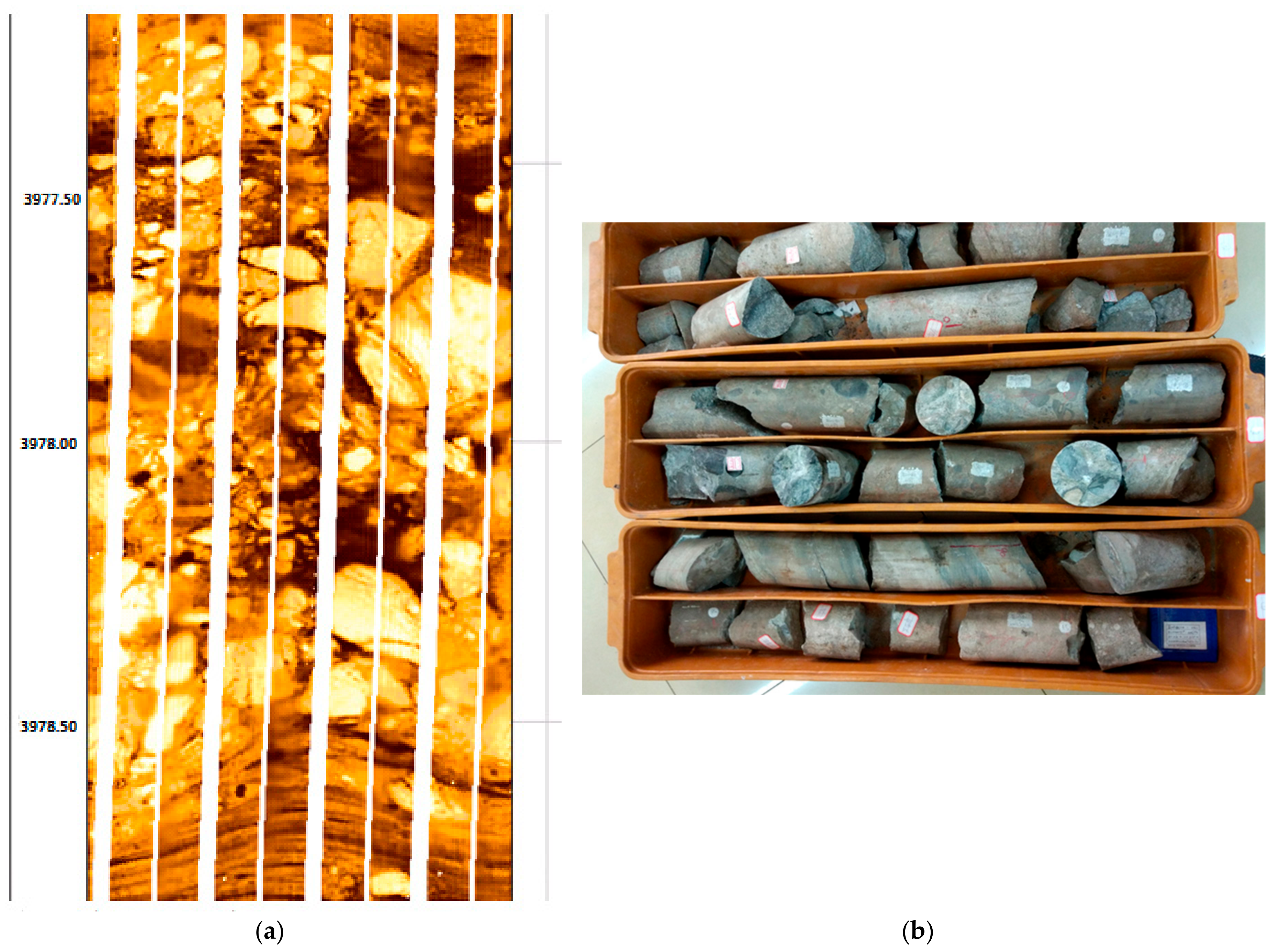
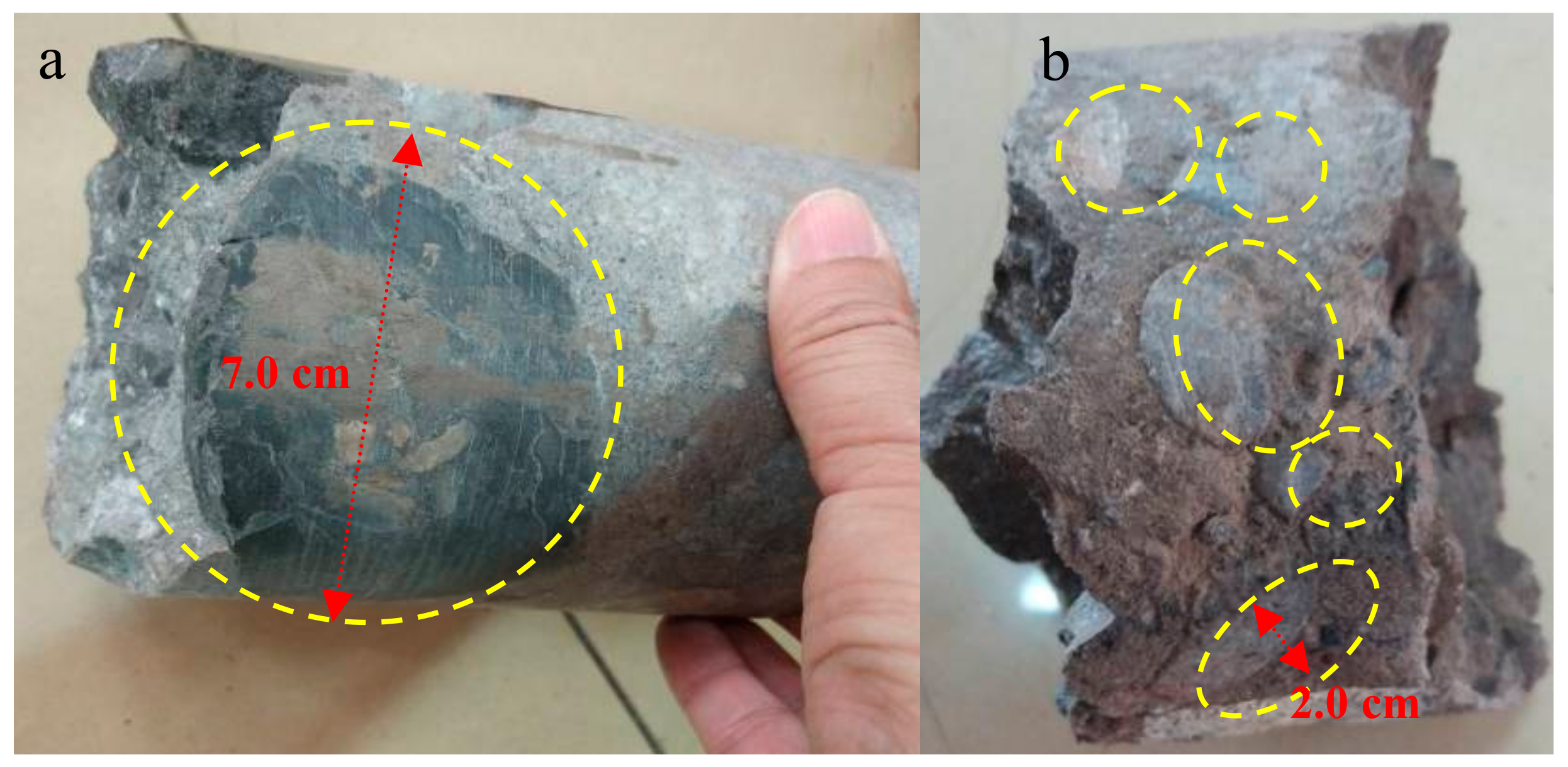
Glutenite reservoirs are typically composed of sandstone and conglomerate gravels which are formed under rapid deposition in nearby provenances [8]. Tight glutenites are among those with low or ultra-low permeability that can range from 0.1 mD to 0.0001 mD [9]. The gravels in the tight glutenites display complex spatial distributions as indicated in Figure 1a which shows the Formation MicroScanner Image (FMI) result in the Ken761 block in Dongying, Shandong province, China [10]. Glutenite cores are drilled for further research and some of them are shown in Figure 1b. From closer observation of the drill cores such as those in Figure 2a,b, glutenites are found to generally develop gravels of irregular shapes, various contents, and different sizes. Since this type of tight reservoir generally develops with low or ultra-low permeability, low porosity and poor connectivity, it is hard to extract the hydrocarbon at a commercial rate without a fracturing operation. The presence of gravels raises the reservoir heterogeneity, complicates the propagation behavior of HFs to exhibit very different characteristics from those in other reservoirs, and makes it difficult to predict the fracture path [11,12].
Due to the random gravel distribution, it is almost impossible to make clear the fracturing behavior of a glutenite reservoir merely through theoretical analysis. On site, HF geometry is inspected indirectly through post-fracturing data acquisition methods such as microseismic monitoring, which is rather rough due to the inability to identify open-mode HFs [13,14], easy contamination by a variety of noises, signal attenuation through thick, faulty or soft formations [15], and common drawbacks in the interpretation of microseismic mapping [16]. Therefore, in view of the monitoring uncertainty and underground invisibility, it is utterly infeasible to obtain uncontroversial answers to this issue from field-monitoring applications.
To deal with this issue, laboratory experiments and numerical simulations are suitable approaches. Previous studies on this issue have been conducted through these two approaches. Laboratory experiment has always been a direct and compelling method to conduct such investigations and valuable related findings have been achieved [8,11,12,17,18,19]. However, similarly, limited by the inner invisibility of a rock specimen and lack of suitable observation methods, in most cases fractured samples after wellbore shut-in are cut open to observe the fracture geometry, which may partly destroy the HF geometry due to the tough manual separation, leave out small HFs or branches, and lead to loss of the emerge of the fracturing process that is quite essential to illuminate problems in some cases. All these technical restrictions and limitations urge the development of numerical tools for careful study. To conduct studies on this issue, numerical modeling tends to be a good choice that is a low-cost tool that can describe in considerable detail the phenomena observed in laboratory experiments and explore the answer in complicated situations that are difficult to carry out in those experiments. However, to date, few numerical models have considered the heterogeneity of rock reservoirs during hydraulic fracturing. In fact, rock is a heterogeneous geological material which contains a different scale of natural weaknesses, such as pores, grain boundaries and pre-existing cracks [20]. Increasing evidence from practical stimulations in the field shows that HFs can initiate and propagate in intricate ways that are highly influenced by the heterogeneity of rock reservoirs [21,22,23,24]. In tight glutenite, extensive material heterogeneity exists not only in the single rock, but in between the two types of rock, i.e., the sandstone and gravel create interrock heterogeneity. How to investigate the reservoir fracturing behavior with the consideration of the intrarock and interrock heterogeneities remains an enormous challenge.
A numerical code, known as rock failure process analysis (RFPA), is applied in this study. Based on a statistical model, RFPA is considered appropriate for modeling heterogeneous material such as rock. When integrated with the digital image processing (DIP) technique, RFPA is able to distinguish sandstone and gravel that show different colors in digital images, and then be applied to establish numerical models for analysis. Numerical investigations in this paper begin with 2D modeling with the consideration of the geostress anisotropy and gravel strength. Then, 3D models are established to further investigate the fracturing behavior in tight glutenite in detail, especially in situations beyond the 2D model’s ability, with the consideration of gravel distribution, gravel size, and axial ratio. The propagation modes are summarized and the corresponding conditions for each mode to occur are then provided.
2. The Digital Image Processing (DIP) Technique in Rock Failure Process Analysis (RFPA) and Rock Heterogeneities
Since a detailed description of the coupled flow-stress-damage (FSD) model of RFPA has been previously presented [25], this section will briefly introduce the DIP technique in RFPA and then illuminate the issue of intrarock and interrock heterogeneities.
2.1. DIP Technique and Integration in RFPA
DIP is a technique used to capture a scene electronically by transforming it into a two-dimensional pixel image and then processing it so as to make the information available for mathematical algorithms [26]. Digital images can be numerically represented in many color systems such as the gray color space, true color space (i.e., the red-green-blue (RGB) space) or the hue, saturation, intensity (HSI) space. It is well known that in the true color space, three independent integer values (R, G and B, from 0 to 255, respectively) are required to describe the red, green and blue level at each pixel. The HSI space is also extensively used due to its close correlation with how humans perceive colors. The hue component H (from 0 to 360) represents the dominant wavelength of the color, which is the domain color feature perceived by humans. The saturation component S (value from 0 to 1) represents the purity of color, defined as how strongly it is polluted with white. The intensity component I (value from 0 to 1) stands for the color brightness or lightness that is unrelated to colors [27]. For convenience to display in the software, the three component variables H, S and I used in this paper are normalized to be from 0 to 255. Digital images can be identified and edited by some image processing tools. With the integration of the DIP technique, RFPA is able to identify the images in BMP (Bitmap) format and then can establish numerical models.
Digital images of rock can be obtained by photographing rock surfaces or the fresh cross-sections of rock samples, or by recovering maps from X-ray Computed Tomography (CT) scanning or other methods [27]. When such a BMP-format image of rock is imported into RFPA, it will be discretized into many square elements of identical size. Each element maps directly onto one finite element that is used for subsequent analysis. It is strongly recommended that the elements number should not be lower than the total image pixels so as to ensure that the element size is not larger than that a pixel represents, thus avoiding a loss of information the pixels contain. Since rock contains a variety of micro-structures (such as minerals, pores, pre-existing cracks, etc.) that may exhibit distinct perceived colors, elements mapping onto these micro-structures can be divided into several groups according to the color data (R, G, B and I) provided in RFPA. The groups number is suggested in agreement with the micro-structures number in cautious research. Once the grouping has been completed, the unique relation between micro-structures and relevant material properties can be established. It is important to note that, in this study, making clear which type each micro-structure in the digital image really is should be done upfront because it is impossible for a software like RFPA to figure out what a micro-structure really is just by their color data. Similarly, the mechanical parameters of micro-structures should be obtained before numerical simulation.
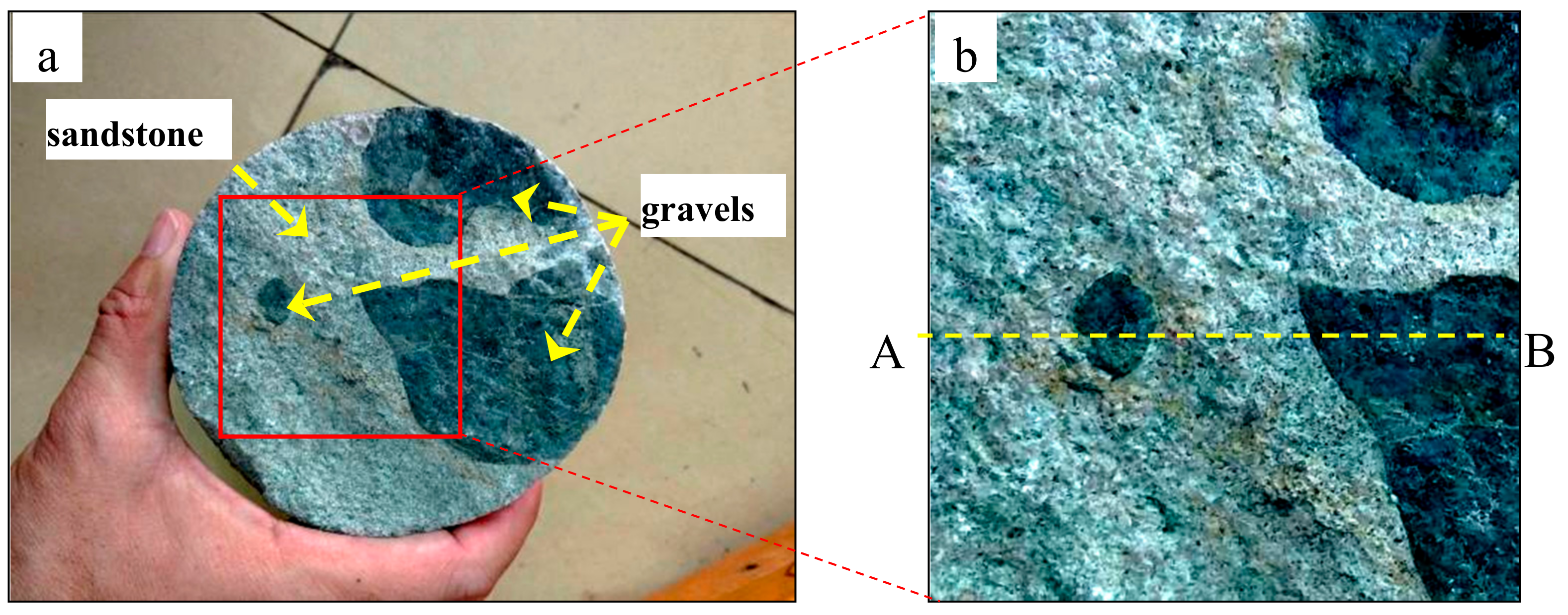
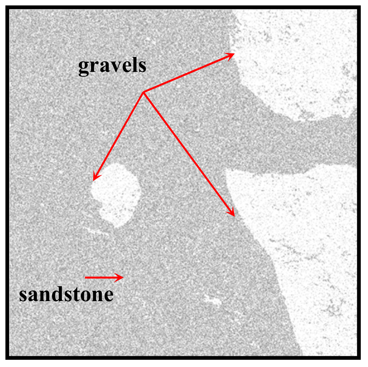
A digital image of a glutenite sample from the Ken761 block in Dongying, Shandong province, China, is shown in Figure 3a, in which a circular cross-section (Diameter: 110 mm) contains two micro-structures: the dark color represents conglomerate gravels and the bright color represents sandstone. A block is cut from the cross-section for analysis, as shown in Figure 3b. It consists of 500 × 500 pixels and the side length is 58 mm.
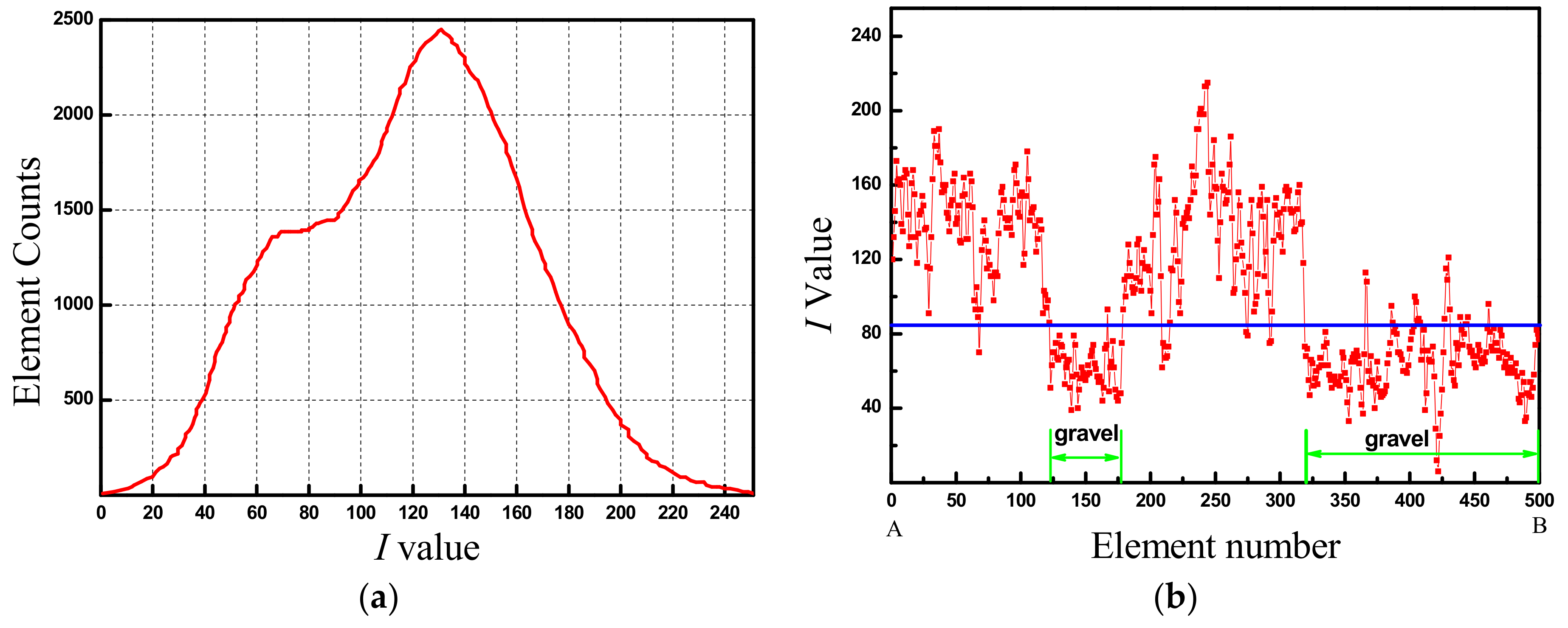
When this block is imported into RFPA, it will be discretized into 500 × 500 finite elements by default, with each pixel transformed into an element. RFPA can capture the color information in the image and then provide to the operator. Since the two micro-structures in the block exhibit distinct difference in brightness, it is quite convenient to divide element groups by the values of I. Figure 4a is a statistical graph provided by RFPA that describes the counts of elements with different I values. Color information of each element can be obtained from RFPA. For example, when an arbitrary line is drawn by the mouse in the RFPA interface, like A–B in Figure 3b, the color information of the elements the line passes will be presented to the operator. Figure 4b describes the I values of the 500 elements along line A–B, from which those in gravel sections are observed generally lower than those in sandstone sections as expected. After several trials, a threshold, 85, at the level that the blue line in Figure 4b denotes, is adopted to divide all the elements into two groups. Elements with I values lesser than 85 are classified into the gravel group and those with I values equal to or larger than 85 are classified into the sandstone group. After assigning reasonable mechanical parameters to the two element groups, the rough sketch of the numerical model will form as shown in Figure 5.
2.2. Intrarock and Interrock Heterogeneities
As one of the most important rock characteristics, heterogeneity significantly influences geostress distribution and rock failure by the existence of different minerals, pores and micro-cracks [28,29]. To numerically represent the influence, a statistical model based on Weibull distribution is introduced into RFPA to take into account this intrarock heterogeneity [30]. A simple numerical model is established in RFPA as shown in Figure 6 to reveal this influence. The rock specimen is 400 mm × 400 mm in size and it is discretized into 400 × 400 finite elements. Constant confining stress, σx (3.0 MPa) and σy (2.0 MPa), is applied to the model boundary. A hole with radius of 15 mm is preset in the center, into which an initial hydraulic pressure of 1.0 Mpa with an increment of 0.05 Mpa per loading step is imposed until the specimen breaks downs. Two cases are set for comparison. Case I: the homogeneity index m is set at 2.0, which represents a large dispersion of material parameters. Case II: the homogeneity index m is set at 20.0, which represents a concentration of material parameters. The rock physico-mechanical parameters are listed in Table 1.
When the initial pressure 1.0 Mpa is imposed on the hole, the radial stress component σr of elements along the dashed radius shown in Figure 6 in the two cases are drawn in Figure 7. The theoretical solution [31] of the same model on homogeneous rock is also drawn for comparison. As shown in the figure, there is a good agreement between the numerical solution in Case II and the theoretical solution except some small fluctuations. However, in Case I, obvious stress fluctuations can be observed, although the average level floats close to the theoretical solution. This phenomenon indicates that rock heterogeneity significantly influences the stress field and that a lower homogeneity index (m) contributes to the larger stress dispersion and vice versa.
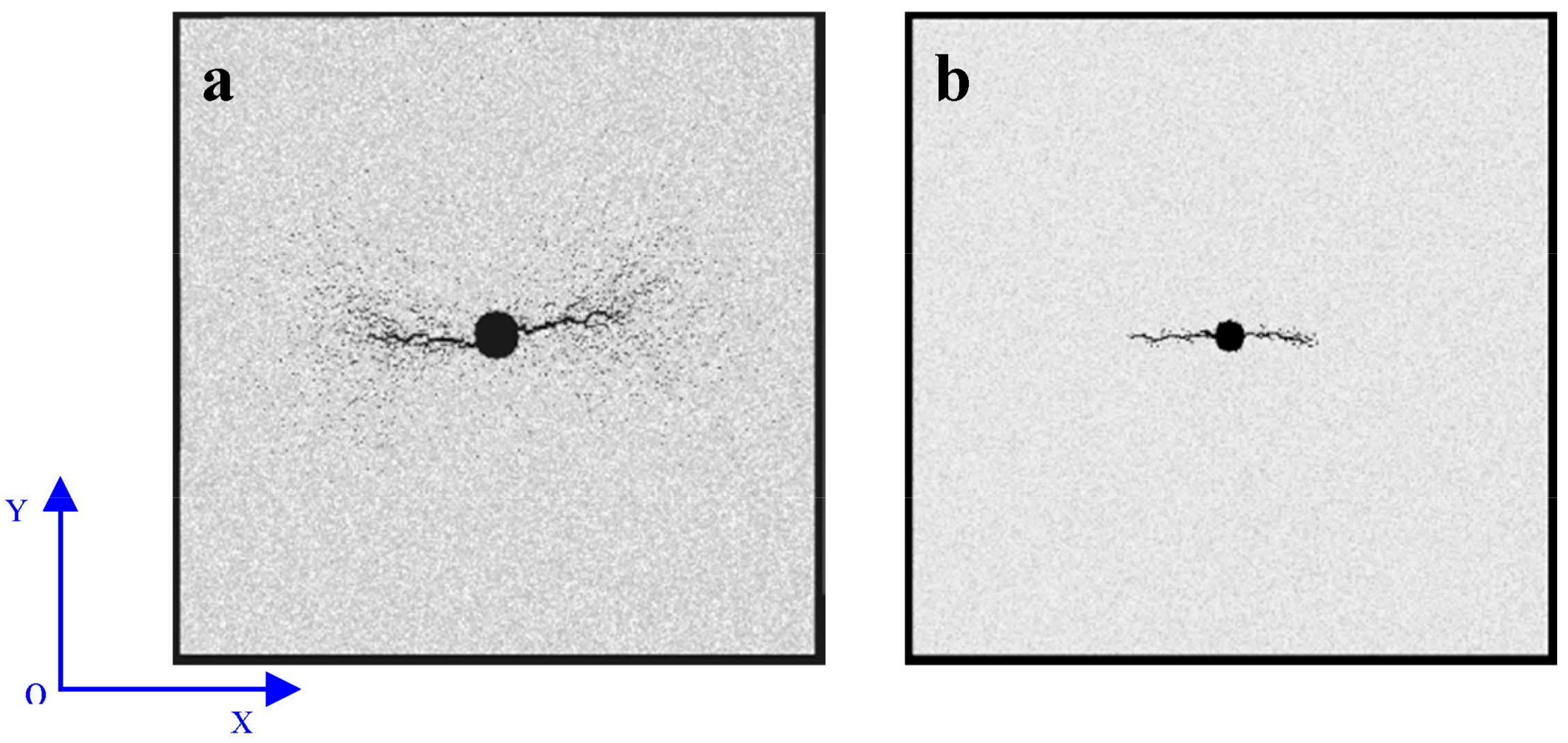
HFs generated in Case I and Case II are shown in Figure 8 (in which pure black elements represent those preset as cavity or have failed in the numerical calculation). Figure 8a reveals HFs in Case I do not rigorously initiate at the hole wall in the maximum principle stress direction, i.e., x axis direction. The right branch deviates slightly from the x axis direction and makes the HFs looks asymmetric. In Case II, as shown in Figure 8b, HFs initiate exactly at the hole wall along the x axis direction and propagate straight to form a typical symmetrical fracture. In Case I, some scattered failed elements are observed to appear on both sides of the HFs while few can be found in Case II. The comparison of the two cases demonstrates rock heterogeneity really influences the rock failure.
In addition to intrarock heterogeneity, problems still exist in formations with variational lithologies such as the glutenite reservoirs. In these formations, multi-types of rock compose the formation and this interrock heterogeneity could also affect significantly rock failure. This is not difficult to understand but how to consider this heterogeneity appropriately is not easy to answer. Fortunately, the DIP technique could help to deal with this task as long as suitable images are available.
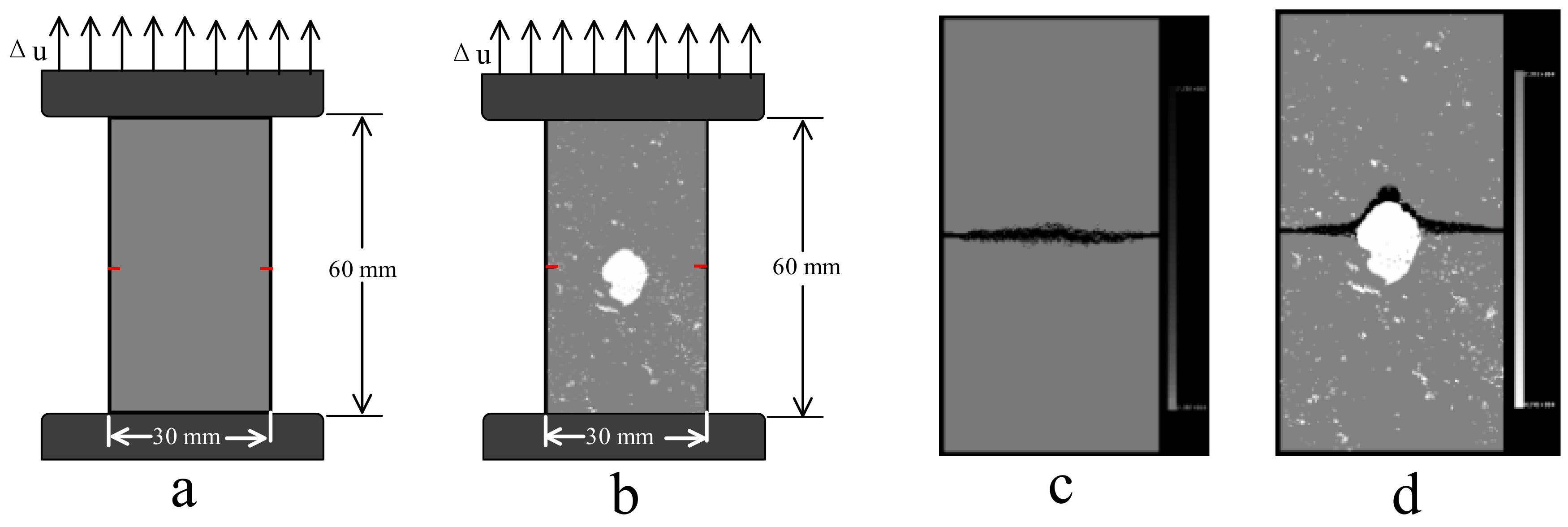
For example, uniaxial tensile numerical tests are conducted in RFPA on a pure sandstone specimen and a glutenite specimen and they are named as Case III and Case IV, respectively. The geometric size and boundary conditions are shown in Figure 9a,b. Each specimen is discretized into 250 × 500 finite elements. The glutenite specimen in Case IV is established in RFPA with the DIP technique from a sub-image from Figure 3a, in which bright regions represent gravel and dark regions represent sandstone. To exclude the influence of intrarock heterogeneity, the homogeneity indices m of both the sandstone and gravel in the two tests are set at 100.0 that is large enough to create a homogeneous material. The rock physico-mechanical parameters are listed in Table 2. Side notches are precut in the specimens as shown in Figure 9a,b so as to preferably catch the gravel effect. An external displacement Δu, at a constant rate of 0.0002 mm/step, is applied on the specimens in the axial direction.
The test results are shown in Figure 9c,d. A common tensile fracture forms in the homogeneous sandstone specimen along the preset notches (Figure 9c). In the glutenite specimen, however, when intersecting the gravel, the tensile fracture tends to deflect and propagate along the sandstone–gravel interface, forming a bending fracture. It can be seen that the glutenite specimen, although composed of homogeneous rocks, exhibits peculiar behavior under tension due to composition of two types of rock. Therefore, the interrock heterogeneity in formations with variational lithologies should be seriously considered and the DIP technique in RFPA can be useful for dealing with similar problems.
In this study, both the glutenite intrarock and interrock heterogeneities are considered in the numerical simulations. The Weibull statistical model is applied to consider the intrarock heterogeneity and each homogeneous index represents a heterogeneity level. The interrock heterogeneity is considered through the application of the DIP technique, which relies mainly on the micro-structures in the digital images. After assigning physico-mechanical parameters and boundary conditions, the heterogeneous glutenite model can be set for calculation.
3. 2D Numerical Investigation
Based on the 2D sketch shown in Figure 5, numerical simulations are conducted in this section to investigate the fracturing behavior in tight glutenites with consideration of the stress anisotropy and rock strength.
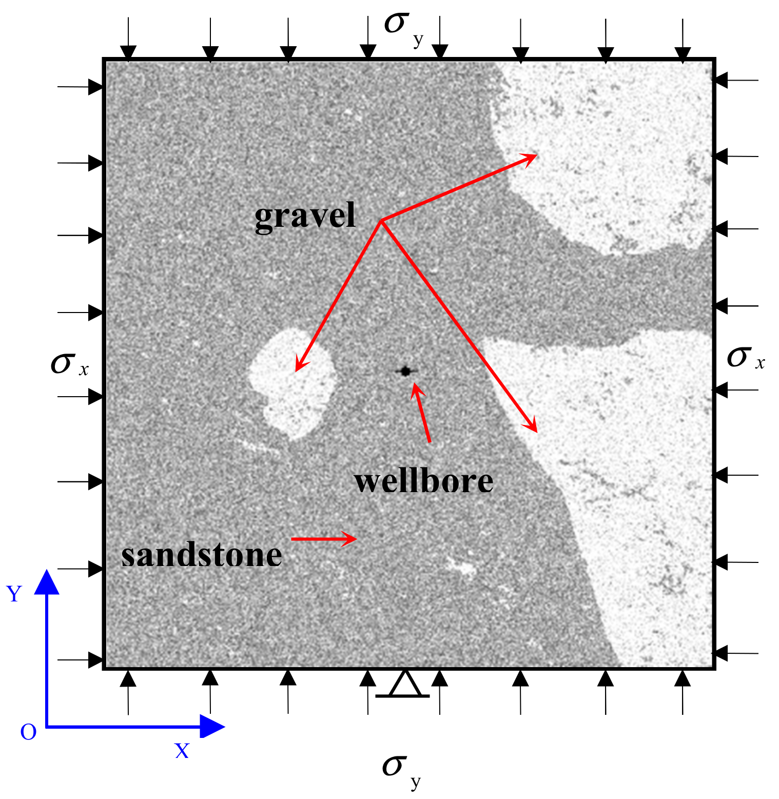
The numerical model is shown in Figure 10, in which a wellbore is preset at the model center with a horizontal perforation. Constant confining stresses, σx and σy, are applied to the model boundaries. The homogeneity indices m of sandstone and gravel are set at 3.0 and 6.0, respectively. Other physico-mechanical parameters are also shown in Table 2. A hydraulic pressure with an increment of 0.1 MPa per loading step is imposed into the wellbore until the specimen breaks down. The model is simplified as a plane strain case during simulation.
3.1. Impact of Stress Anisotropy
Geostress has been confirmed by numerous studies to be a key factor dominating HF propagation [32,33,34,35,36]. Stress anisotropy is crucial for fracturing treatment optimization because HFs always prefer to propagate in the maximum principal stress direction. Therefore, the stress anisotropy should be seriously considered during hydraulic fracturing. In this study, the horizontal stress difference Δσ, defined as Δσ = σx − σy, is applied to quantify the magnitude of stress anisotropy in the numerical model. Base on the stress difference, three numerical cases (A, B and C) as shown in Table 3 are set for simulation.
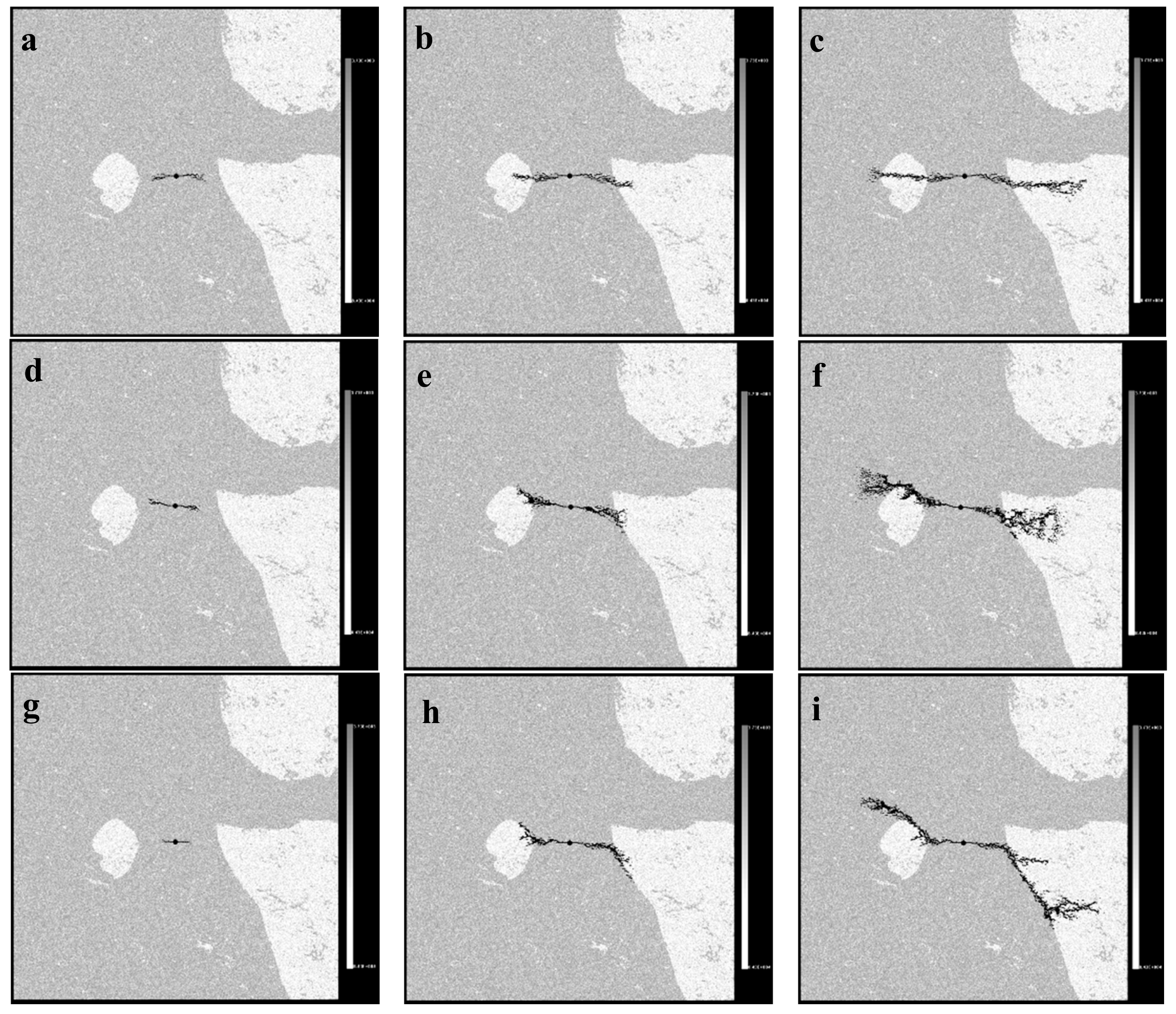
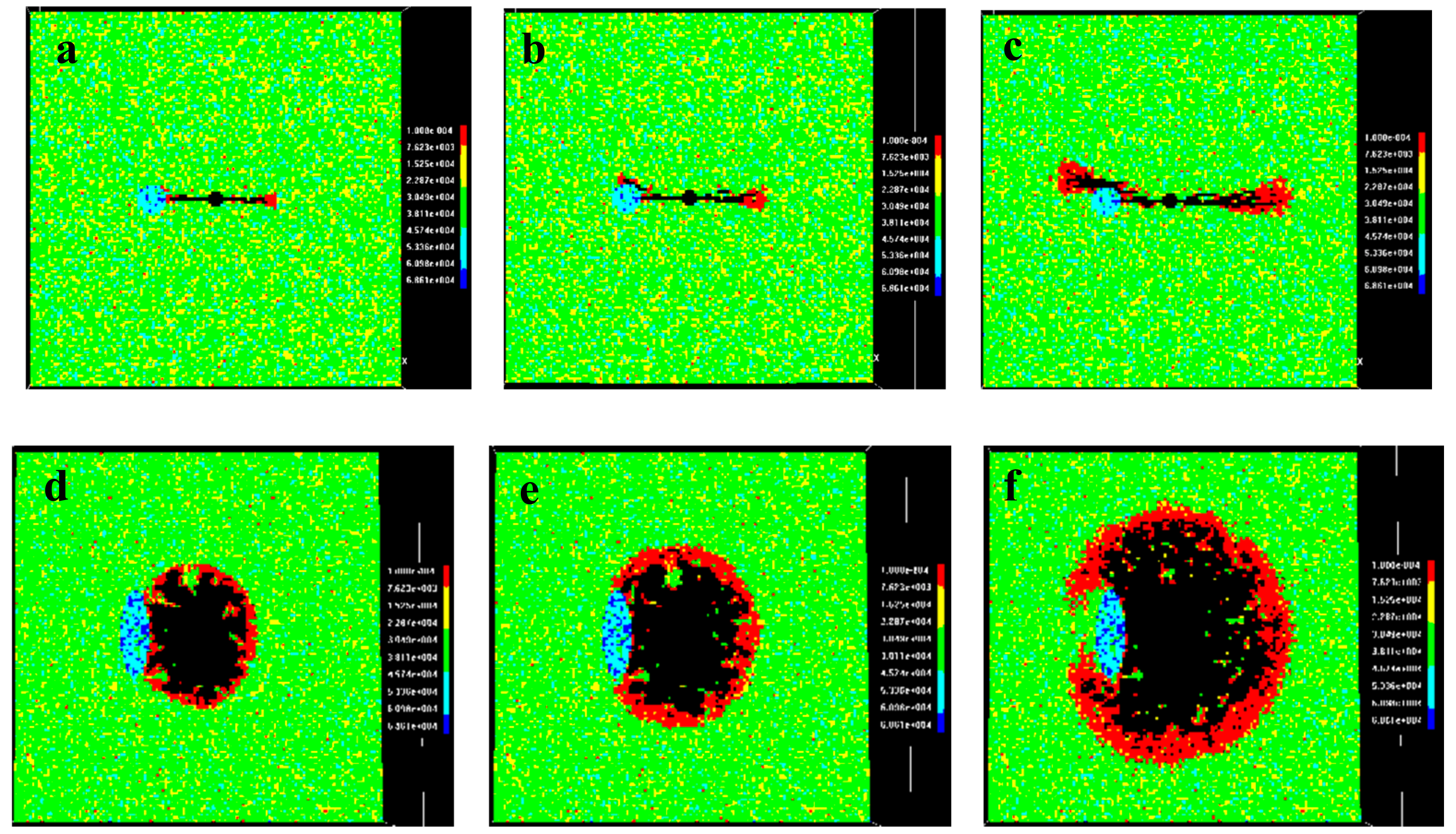
To display the fracturing process and HF geometries in detail, three pictures in each case are selected and shown in sequence in Figure 11a–c corresponding to those in Case A. Figure 11 d–f correspond to those in Case B. Figure 11g–i correspond to those in Case C.
In Case A, HFs initiate from the perforations in both sides and then propagate in the maximum horizontal stress direction, i.e., the x axis direction (Figure 11a). When intersecting the gravels, the HFs exhibit no obvious change in the path and continue to propagate into the gravels or penetrate the gravels (Figure 11b,c). During the entire process, the HFs propagate with no deflection and the gravels exert little influence on the propagation path.
Compared with that in Case A, the stress difference Δσ decreases in Case B, and its control on the HFs propagation attenuates. On this occasion, the effect of rock heterogeneity is enhanced. That is why the initial HFs propagate in not as straight a way as that in Case A (Figure 11d). When intersecting the gravels, the left HF is observed to be deflected from its previous direction and propagates along the gravel until reorientating into its previous direction once again for propagation (Figure 11e,f). In this situation, the gravels act as obstacles for HF propagation. The right HF propagates into the gravel after a small deflection along the gravel (Figure 11f) and then bifurcates into multi-fractures. It should be specially explained that the gravels in the model are not totally monolithologic due to existence of interior defects that exhibit darker color than surrounding gravel elements (Figure 10). In reality, conglomerate gravels generally contain geological defects such as pores, fissures and fillings [37,38]. These defects could complicate the HFs path in gravels.
In Case C, the horizontal stress difference Δσ is the lowest and its control is the weakest. The gravel still acts as obstacle for the left HF (Figure 11g,h). The difference is that, after deflection along the gravel, the left HF reorientates more slowly to the previous direction (Figure 11i), leading to a larger reorientation distance than that in Case B. In addition, the right HF deflects to propagate along the gravel, with new branches extending into the gravel and propagating along the preexisting defects, forming complex multi-fractures.
Therefore, the fracturing operation in tight glutenite could generate HFs with different degrees of complexity, from a single HF as in case A to complex multi-fracture as in Case C, relying on the stress anisotropy. A higher stress difference Δσ facilitates the HFs to penetrate through the gravels and induces simplex HFs. A lower Δσ usually leads to fracture deflections and bifurcations, resulting in multi-fractures or fracture networks that create higher connectivity among pores and offer easier pathways for the hydrocarbon to move towards the wellbore.
3.2. Impact of Gravel Strength
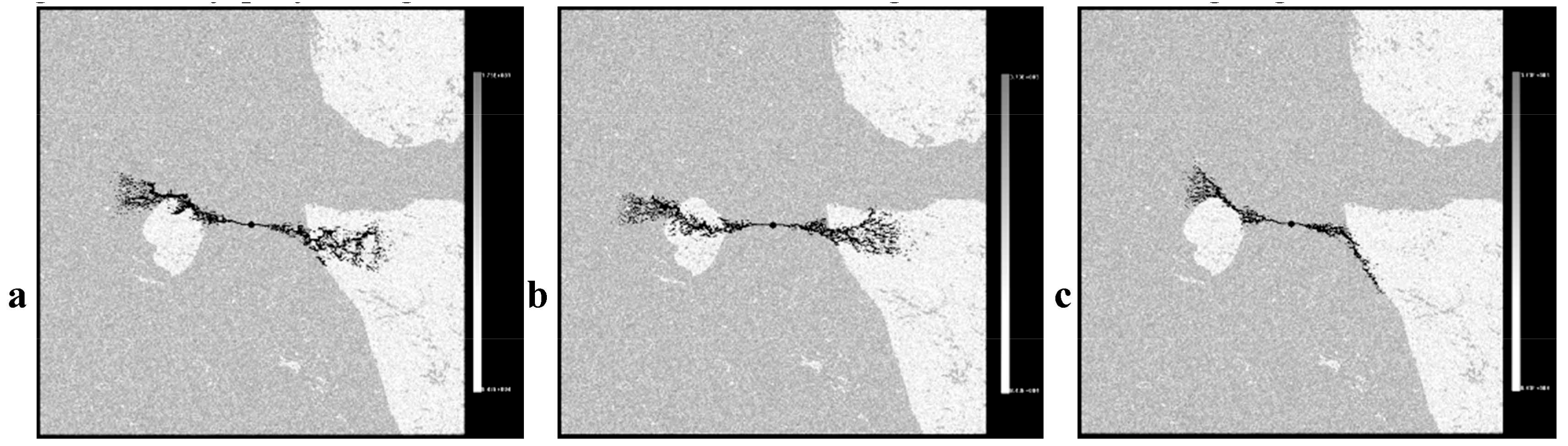
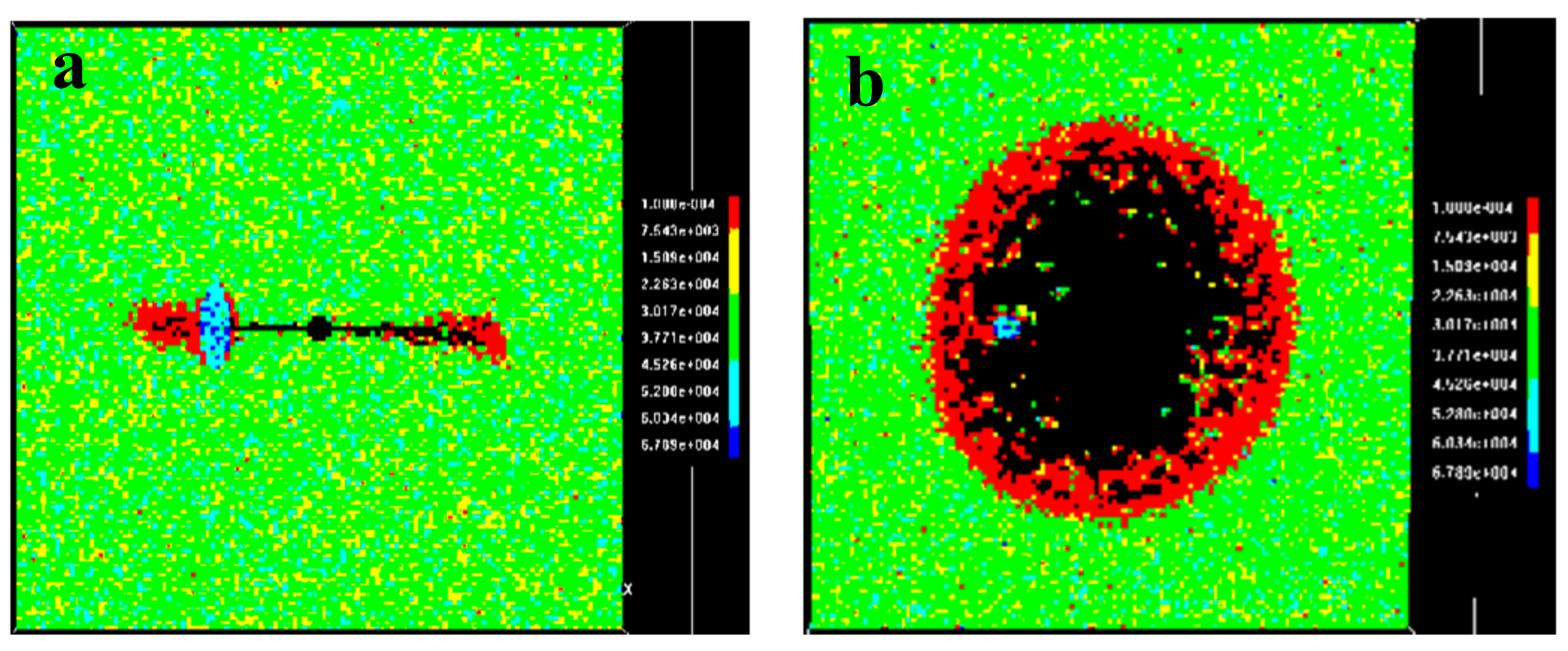
Due to differences in mineral composition, gravels even in the same glutenite reservoir can exhibit distinct strengths. For example, Ma et al. [8] observed two types of gravels in the glutenite specimens marked by gravel (A) and gravel (B). The brown-red gravel (B) containing a high amount of quartz has more than three times the tensile strength of the caesious gravel (A) containing a high amount of feldspar. To consider this gravel strength in this study, Case D and Case E are set for simulation by merely changing the gravel strength to compare with Case B. The gravel uniaxial compressive strength (fc0) decreases to 60.0 MPa in Case D and increases to 200.0 Mpa in Case E compared with the 130.0 MPa in Case B, while keeping the ratio of compressive and tensile strength constant. The obtained HFs geometries in the three cases are shown in Figure 12. Obviously, the HFs are observed to penetrate the gravels with low strength (Figure 12b, Case D) but entirely deflect to propagate along the gravels with high strength (Figure 12c, Case E). The gravel strength actually plays a significant role in the fracturing behavior of the tight glutenite reservoirs.
4. 3D Numerical Investigation
The propagation of HFs in tight glutenites can be simplified as a 2D model in some cases, but in some other cases a 3D model is essential because of the unique gravel characteristic such as gravel shape. This section focuses on the fracturing behavior in tight glutenites through 3D simulation. Numerous studies indicate conglomerate gravels are of various shapes and sizes. The gravels generally develop in quasi-spheroidal, ellipsoidal or irregular shapes. The gravel size, taking the Daxing conglomerate, for example [37], can range from 2 cm to 20 cm, and some big gravels can reach several dozen centimeters or even a few meters. Both the gravel shape and size can affect the HF propagation and geometry. In addition, the gravel distribution, which determines the positional relation of the gravel and the HF, is also considered in the numerical model.
4.1. The 3D Numerical Model
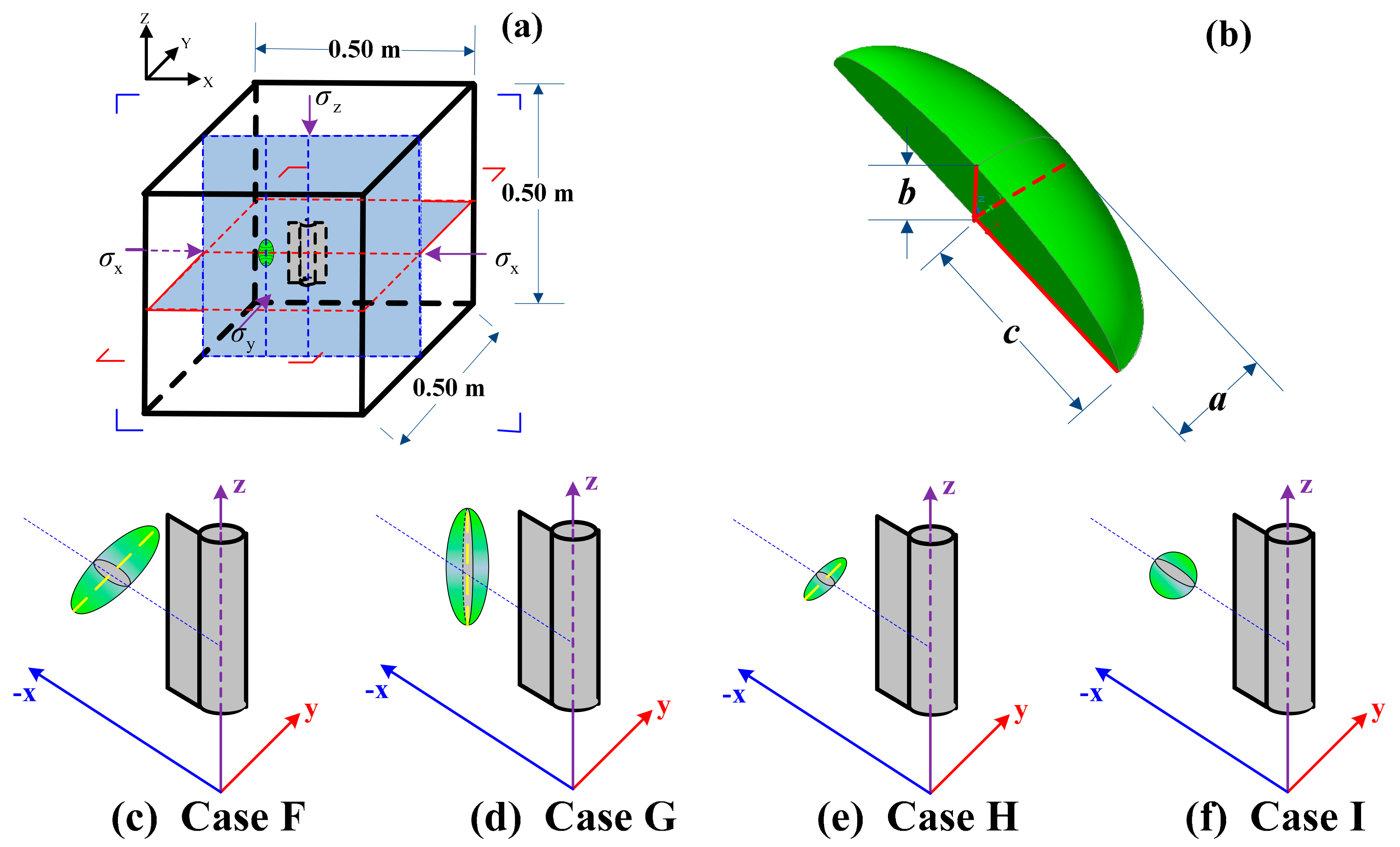
A 3D numerical model is established in RFPA with the sketch illustrated in Figure 13a. A cubic glutenite specimen, whose side length is 0.50 m, is discretized into 1,953,125 (125 × 125 × 125) finite elements. A wellbore, 0.024 m in diameter and 0.10 m in depth, into which an initial hydraulic pressure (20.0 MPa) with an increment (0.1 MPa per loading step) is imposed, is preset vertically (the wellbore axis is parallel to the z axis in the Cartesian coordinate system) at the cube center. Notches are precut on both sides of the borehole along the x axis as perforations. σx (30.0 MPa), σy (20.0 MPa) and σz (32.0 MPa), which represent the three principal stresses, are applied to the model boundaries. An ellipsoidal gravel locates in the cubic and its axial size is expressed by a, b and c (Figure 13b). The gravel shape and size change as the three variables change. For simplification, a and b are set equal in the model. Therefore, a (or b) and c are independent variables to control the gravel shape and size. Four numerical cases (Case F, G, H and I) are established according to the gravel characteristic with detailed description illustrated in Figure 13c–f and Table 4. The homogeneity indices m of sandstone and gravel are still set at 3.0 and 6.0, respectively. The gravels are all assigned with high strength (fc0 = 200.0 MPa, the same as in Case E) that are not easily destroyed under hydraulic pressure compared with sandstone. All the other physico-mechanical parameters are also shown in Table 2.
4.2. Results and Discussion
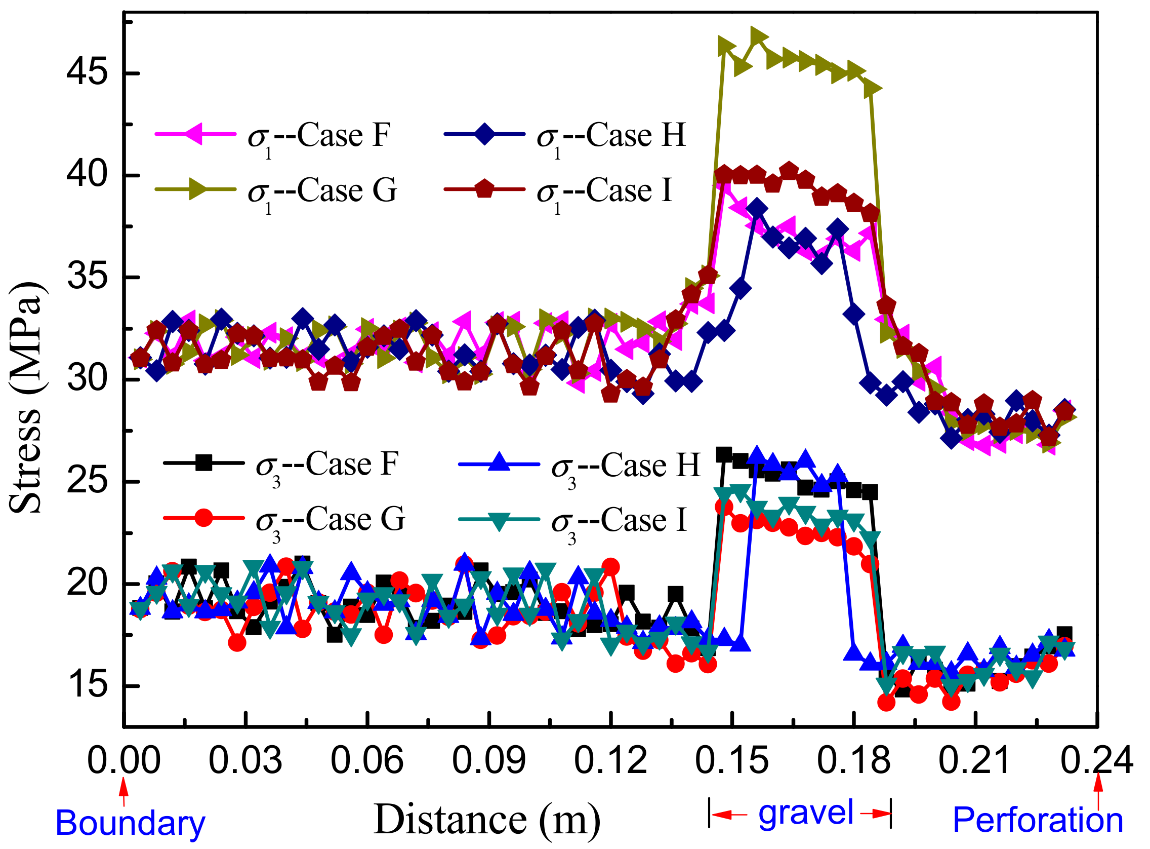
As the initial hydraulic pressure 20.0 MPa is imposed on the wellbore, the maximum principal stress σ1 and the minimum principal stress σ3 of model elements in Case F, G, H and I along the blue dashed lines in Figure 13c–f, respectively, are shown in Figure 14 in which the model boundary element is set as the abscissa origin and the perforation locates in the positive horizontal direction. This demonstrates that the principal stresses of sandstone elements in the four cases are nearly equal to each other and they exhibit some fluctuations. However, both the two principal stresses of gravel elements are found to be much higher than those of sandstone elements and they exhibit smaller fluctuations. The gravel differences in the four cases lead to stress differences in gravel elements and the cases (G and I) with higher values of σ1 are observed to have lower values of σ3.
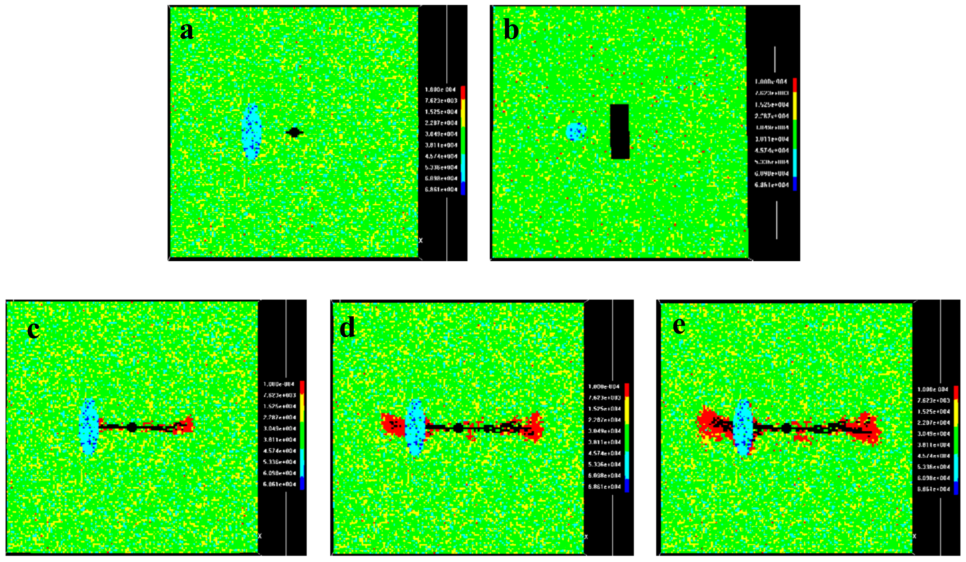
To inspect the fracturing behavior carefully, a cross section and a longitudinal section both passing the cube center are selected for description (Figure 13a). Figure 15a,b, respectively, shows the cross section and the longitudinal section in Case F before fracturing. Elements in the figures exhibiting cool colors like blue or green represent materials with high Young’s modulus while those exhibiting warm colors like red or orange represent materials with low Young’s modulus. The gravel exhibits the coolest colors and can be easily distinguished from the sandstone. The HF propagation process in Case F is shown in Figure 15c–h, in which c, d and e correspond to the cross sections and f, g and h correspond to the longitudinal sections in the same loading steps as in the cross sections.
The HFs initiate from the perforations and extend in both length and height. Once intersecting the gravel, the fracture section right ahead the gravel stops but the sections above and below the gravel continue to propagate, as revealed in Figure 15c,f. Afterwards, the upper section radiates downwards and the lower section radiates upwards, leading to the coalescence behind the gravel (Figure 15d,g). In this manner, a bypass HF forms with the final geometry shown in Figure 15e,h.
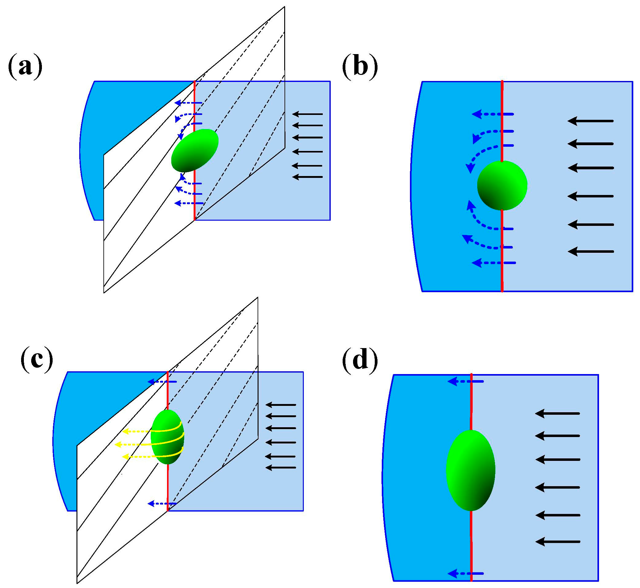
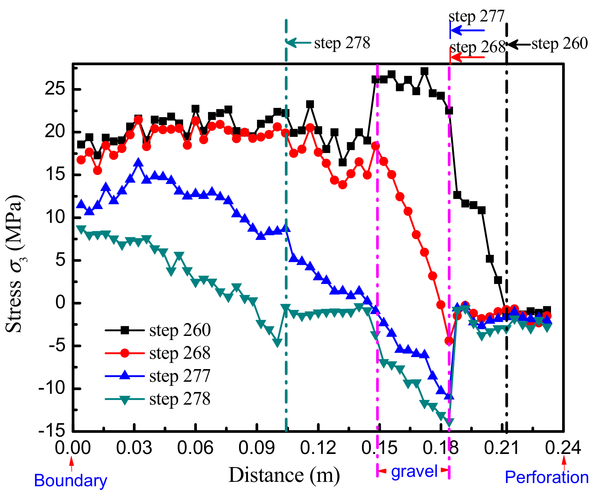
The diagrams in Figure 16a,b illustrate the formation of the bypass HF in Case F. Light and dark blue regions represent the fracture plane in front of the gravel and its extended plane behind the gravel, respectively. The white region shows the plane orthogonal to the blue region. Their intersecting line is highlighted in red. The black and blue arrows show the directions of the HF extending out from the wellbore and near the gravel, respectively. The 3D view and front view describe the HF path when intersecting the gravel. The gravel prevents the propagation of the HF right ahead but the upper and lower sections continue to propagate past the gravel. Then the upper and the lower sections radiate to coalesce and attain a full fracture height behind the gravel. This process can also be reflected through the stress evolution in Figure 17, in which the minimum principal stresses σ3 of elements along the blue dashed line in Figure 13c in four loading steps are recorded. In step 260, the HF propagates to the location 0.212 m away from the boundary, before intersecting the gravel. Elements stress σ3 before the HF are large enough to reach the tensile failure threshold (sandstone: −ft0 = −4.5 MPa; gravel: −ft0 = −20.0 MPa). In step 268, the HF propagates to exactly intersect the gravel. The stress σ3 of elements just before the HF, i.e., the gravel elements stress σ3, decrease dramatically from that in step 260. Afterwards, in step 277, both sandstone and gravel elements stress σ3 before the HF continues to decrease but there are still no more failure elements in the figure because no more elements’ stress σ3 reach the threshold. In reality, this step is the time when the upper and lower HFs propagate past the gravel and radiate before coalescence. In step 278, the HF has bypassed the gravel and propagated to the location 0.104 m away from the boundary, with the stress σ3 of sandstone elements before the HF building up, reaching the failure threshold and transferring to surrounding elements. This cyclic process of stress buildup and transfer signifies the continuous HF propagation. It is important to note that the gravel elements stress σ3 keep above the gravel tensile failure threshold during the simulation. That is why the gravel in Case F remains unbroken in the whole fracturing process, as shown in Figure 15.
This bypass HF exhibits unique characteristic and its formation is quite different from those in conventional reservoirs. Firstly, this fracturing process contains not only the common process of outward fracture propagation in fracture length and height but also the regional process of fracture stop, inward radiation and coalescence. This behavior must be interpreted with caution through 3D simulations since this bypass facture is formed through complex 3D growth and cannot be captured in a 2D simulation. Secondly, the final HF is observed to be cut off at the gravel and it is discontinuous (Figure 15e). From the 2D view, the HF can actually propagate regularly with no deflection after bypassing the gravel in the 3D model. After the bypass, the gravel appears be embedded into the sandstone at two sides of the HF, with only the circle edge the HF bypasses are exposing in the fracturing fluid. On this occasion, even though at the time when the HF has completely penetrated the cube boundaries, it is still difficult to separate the cube specimen along the HF because the gravel embedded into the sandstone has not broken. However, in most laboratory experiments, the fractured specimens are often separated along the main HF by manual operation to observe the inner HF geometry. This operation, unfortunately, may break the gravel along the HF section or strip the gravel at the sandstone-gravel interface, which may be mistaken as evidences for the HF directly penetrating the gravel or deflecting to propagate along the interface, respectively. In reality, this operation has disturbed the observer’s decision on the mode the HFs form in when they intersect gravels. This might partly be the reason why this mode of HF propagation is rarely stated during previous experiments.
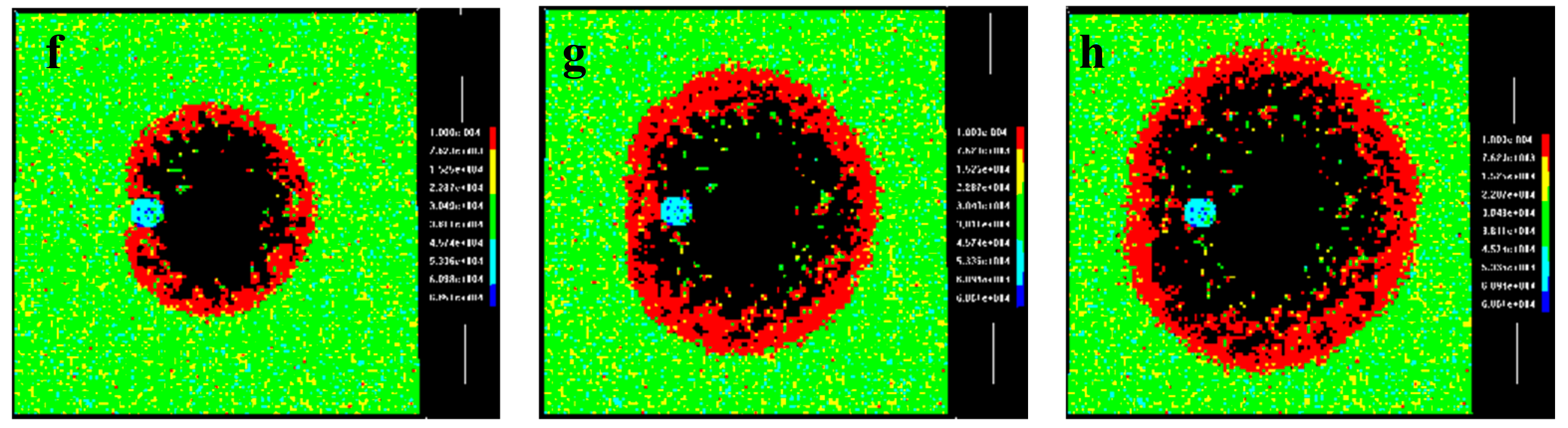
The gravel in Case G changes only the distribution orientation with the long axis parallel to the z axis, compared with that in Case F. However, just such a small change leads to totally different simulation results as shown in Figure 18. When intersecting the gravel, the HF section right ahead of the gravel deflects to propagate (Figure 18a–c) while the upper and lower sections maintain their previous direction to propagate over the gravel with no deflection (Figure 18d–f). This process is illustrated in the diagrams in Figure 16c,d where the yellow arrows show the directions of HF deflections. The gravel merely deflects the HF section right ahead, ultimately resulting in a distorted HF.
Compared with Case F, the gravel in Case H simply develops with a smaller size. The final HF geometries in Case H are shown in Figure 19a,b. It is easy to see that the HF propagates past the gravel with no deflection and it is a bypass fracture which is similar to that in Case F.
In Case I, the axial ratio decreases to 1 and the gravel is actually a sphere. The final HF geometries in Case I are shown in Figure 19c,d. When intersecting the gravel, the HF right ahead the gravel bifurcates into two branches which deflect to propagate along the gravel. In this manner a distorted HF forms. The propagation mode is similar to that in Case G.
Some findings can be obtained from the comparison of the four numerical cases above. By comparing Cases F and H, in which the gravels share the same distribution orientation and axial ratio but different sizes, it can be seen that pure gravel size within certain limits has little impact on the propagation mode of HFs when intersecting gravels, since the HFs in the two cases show similar behavior under considered conditions. Similarly, by comparing Cases F and G, and Cases F and I, where HFs exhibit different behavior, the impacts of gravel distribution orientation and axial ratio are verified. When the gravel’s long axis locates in agreement with the HF width, HF is preferential to bypass the gravel with no deflection, or penetrate the gravel directly in situations such as in Case A where the gravel strength is not as high as in the 3D simulations. When the gravel axial ratio decreases, for example, from 3 in Case F to 1 in Case I, the HFs deflect to propagate when intersecting the gravel. This phenomenon indicates a rounder gravel, i.e., a lower axial ratio, creating better opportunities for HFs deflection.
Through further analysis, the authors attribute the impacts of factors such as gravel distribution orientation and axial ratio to the competition of the gravel size in the HF height direction with that in the width direction. When the gravel size in the HF width direction prevails, it is easier for HFs to penetrate or bypass the gravel than to deflect to propagate for a long distance, because the vast majority of the fracturing fluid will still flow into the main fracture after passing the gravel, rather than flow into the tortuous path of the deflected fracture. Otherwise, HFs will deflect for some distance to propagate along the gravels, especially in situations when the gravels develop weak interfaces.
In summary, the propagation modes of HFs intersecting gravels in glutenite reservoirs are as follows:
- (1)
- Penetrating directly.
- (2)
- Deflecting to propagate along the gravels to form distorted HFs.
- (3)
- Propagating to bypass the gravels.
- (4)
- Combination of (1) and (2), or (2) and (3).
in which mode (1) prefers to occur in situations when the horizontal stress difference is high, the gravel strength is not large, and the gravel size along the HF width direction is not small; mode (2) prefers to occur when the horizontal stress difference is low, the gravel strength is large, and the gravel size along the HF width direction is not large; mode (3) prefers to occur when the horizontal stress difference is high, the gravel strength is large, and the gravel size along the HF width direction is not small; mode (4) occurs in situations at the intermediate levels correspond to (1) and (2), or (2) and (3), or when the gravels develop interior weaknesses.
5. Conclusions
This paper provides a numerical method to investigate fracturing behavior in tight glutenites. The DIP technique and its integration into RFPA are briefly introduced. Glutenite heterogeneities, including intrarock heterogeneity and interrock heterogeneity, are considered to affect HF propagation. RFPA is capable of considering the intrarock heterogeneity by applying the Weibull model and the interrock heterogeneity with the import of suitable images when integrated with the DIP technique. Its practicability is verified through numerical simulations of hole hydraulic fracturing tests and uniaxial tension tests that have simultaneously confirmed the significant influence of intrarock and interrock heterogeneities on rock stress and failure.
A section image of a glutenite sample was imported into RFPA for a 2D fracturing simulation. Results show that when intersecting the gravel, the HFs can penetrate or deflect, depending on the magnitude of stress anisotropy and gravel strength. A higher horizontal stress difference drives the HFs to directly penetrate the gravel, forming simplex fractures. While a lower horizontal stress difference encourages the HF to deflect along gravels, forming complex fractures. Gravels with interior defects provide opportunities to form complex multi-fractures. Gravels with high strength will behave as obstacles for HFs to penetrate and vice versa.
3D simulations are conducted with the consideration of gravel distribution, gravel size and axial ratio. HFs could propagate past the gravel with no deflection, forming a bypass fracture, which is not easy to observe in common laboratory experiments. They can also deflect to propagate along the gravels like in the 2D simulations. The impact of the gravel distribution orientation and the axial ratio are attributed to the competion of gravel size in the HF height direction with that in the width direction, through which the propagation behaviors of HFs intersecting the gravels can be clarified.
The propagation modes of HFs intersecting gravels in tight glutenite are summarized as: (1) penetrating directly; (2) deflecting to propagate along the gravels to form distorted HFs; (3) propagating to bypass the gravels; (4) a combination of (1) and (2), or (2) and (3). The corresponding conditions for each mode to occur are provided. This study is expected to shed light on the fracturing behavior of tight glutenites during hydraulic stimulations.
Author Contributions
Conceptualization, Z.L.; Methodology, L.L. and Z.Z.; Investigation, M.L.; Formal analysis, L.Z.; Validation, B.H.; Software, C.T.; Writing—Original Draft, Z.L.; Writing—Review and Editing, L.L.
Funding
The authors acknowledge support from the grants from National Science and Technology Major Project (Grant No. 2017ZX05072), National Natural Science Foundation of China (Grant Nos. 51761135102 and 51479024) and Anhui Province Science and Technology Project of China (Grant 17030901023).
Conflicts of Interest
The authors declare no conflict of interest.
References
- Weng, X.; Kresse, O.; Chuprakov, D.; Cohen, C.-E.; Prioul, R.; Ganguly, U. Applying complex fracture model and integrated workflow in unconventional reservoirs. J. Petroleum Sci. Eng. 2014, 124, 468–483. [Google Scholar] [CrossRef]
- Zou, Y.; Zhang, S.; Zhou, T.; Zhou, X.; Guo, T. Experimental Investigation into Hydraulic Fracture Network Propagation in Gas Shales Using CT Scanning Technology. Rock Mech. Rock Eng. 2015, 49, 1–13. [Google Scholar]
- Dehghan, A.N.; Goshtasbi, K.; Ahangari, K.; Jin, Y.; Bahmani, A. 3D Numerical Modeling of the Propagation of Hydraulic Fracture at Its Intersection with Natural (Pre-existing) Fracture. Rock Mech. Rock Eng. 2016, 50, 1–20. [Google Scholar] [CrossRef]
- Fu, W.; Ames, B.C.; Bunger, A.P.; Savitski, A.A. Impact of Partially Cemented and Non-persistent Natural Fractures on Hydraulic Fracture Propagation. Rock Mech. Rock Eng. 2016, 49, 4519–4526. [Google Scholar] [CrossRef]
- Huang, B.; Liu, J. Experimental Investigation of the Effect of Bedding Planes on Hydraulic Fracturing under True Triaxial Stress. Rock Mech. Rock Eng. 2017, 50, 2627–2643. [Google Scholar] [CrossRef]
- Liu, Z.; Wang, S.; Zhao, H.; Wang, L.; Li, W.; Geng, Y.; Tao, S.; Zhang, G.; Chen, M. Effect of Random Natural Fractures on Hydraulic Fracture Propagation Geometry in Fractured Carbonate Rocks. Rock Mech. Rock Eng. 2017, 51, 491–511. [Google Scholar] [CrossRef]
- Llanos, E.M.; Jeffrey, R.G.; Hillis, R.; Zhang, X. Hydraulic Fracture Propagation through an Orthogonal Discontinuity: A Laboratory, Analytical and Numerical Study. Rock Mech. Rock Eng. 2017, 50, 2101–2118. [Google Scholar] [CrossRef]
- Ma, X.; Zou, Y.; Li, N.; Chen, M.; Zhang, Y.; Liu, Z. Experimental study on the mechanism of hydraulic fracture growth in a glutenite reservoir. J. Struct. Geol. 2017, 97, 37–47. [Google Scholar] [CrossRef]
- Zhu, W.; Wang, Z.; Li, A.; Gao, Y.; Yue, M. The Seepage Theory and Exploitation Technology of Hydraulic Fracturing in Thin Interbed Tight Reservoirs; Science Press: Beijing, China, 2016. [Google Scholar]
- Li, L. Size Effect Tests and Mechanical Properties of Low-Permeability Sandstone under Static and Dynamic Loadings; Shengli Oilfield Branch Company: Dongying, China, 2017. [Google Scholar]
- Meng, Q.M.; Zhang, S.C.; Guo, X.M.; Chen, X.H.; Zhang, Y. Aprimary investigation on propagation mechanism for hydraulic fractures in Glutenite formation. J. Oil Gas Technol. 2010, 32, 119–123. [Google Scholar]
- Li, L.; Meng, Q.; Wang, S.; Li, G.; Tang, C. A numerical investigation of the hydraulic fracturing behaviour of conglomerate in Glutenite formation. Acta Geotech. 2013, 8, 597–618. [Google Scholar] [CrossRef]
- Warpinski, N.R.; Mayerhofer, M.J.; Agarwal, K.; Du, J. Hydraulic fracture geomechanics and microseismic source mechanisms. In Proceedings of the SPE Annual Technical Conference and Exhibition (ATCE2012), San Antonio, TX, USA, 8–10 October 2012. [Google Scholar]
- Haddad, M.; Sepehrnoori, K. XFEM-Based CZM for the Simulation of 3D Multiple-Cluster Hydraulic Fracturing in Quasi-Brittle Shale Formations. Rock Mech. Rock Eng. 2016, 49, 4731–4748. [Google Scholar] [CrossRef]
- Ziarani, A.S.; Chen, C.; Cui, A.; Quirk, D.J.; Roney, D. Fracture and wellbore spacing optimization in multistage fractured horizontal wellbores: Learnings from our experience on Canadian unconventional resources. In Proceedings of the International Petroleum Technology Conference (IPTC2014), Kuala Lumpur, Malaysia, 10–12 December 2014. [Google Scholar]
- Cipolla, C.; Weng, X.; Mack, M.; Ganguly, U.; Gu, H.; Kresse, O.; Cohen, C.E. Integrating microseismic mapping and complex fracture modeling to characterize fracture complexity. In Proceedings of the SPE Hydraulic Fracturing Technology Conference and Exhibition (HFTC2011), The Woodlands, TX, USA, 24–26 January 2011. [Google Scholar]
- Zhao, Z.; Guo, J.; Ma, S. The Experimental Investigation of Hydraulic Fracture Propagation Characteristics in Glutenite Formation. Adv. Mater. Sci. Eng. 2015, 2015, 1–5. [Google Scholar] [CrossRef]
- Ju, Y.; Liu, P.; Chen, J.; Yang, Y.; Ranjithd, P.G. CDEM-based analysis of the 3D initiation and propagation of hydrofracturing cracks in heterogeneous glutenites. J. Nat. Gas Sci. Eng. 2016, 35, 614–623. [Google Scholar] [CrossRef]
- Li, N.; Zhang, S.; Ma, X.; Zou, Y.; Chen, M.; Li, S.; Zhang, Y. Experimental study on the propagation mechanism of hydraulic fracture in glutenite formations. Chin. J. Rock Mech. Eng. 2017, 36, 2383–2392. (In Chinese) [Google Scholar]
- Wang, R.Q.; Kemeny, J.M. A study of the coupling between mechanical loading and flow properties in tuffaceous rock. In Proceedings of the 1st North American Rock Mechanics Symposium, Austin, TX, USA, 1–3 June 1994. [Google Scholar]
- Mahrer, K.D. A review and perspective on far-field hydraulic fracture geometry studies. J. Pet. Sci. Eng. 1999, 24, 13–28. [Google Scholar] [CrossRef]
- Beugelsdijk, L.J.L.; De Pater, C.J.; Sato, K. Experimental hydraulic fracture propagation in a multi-fractured medium. In SPE Asia Pacific Conference on Integrated Modelling for Asset Management; SPE 59419; Society of Petroleum Engineers: Richardson, TX, USA, 2000. [Google Scholar]
- Jeffrey, R.G.; Bunger, A.; LeCampion, B.; Zhang, X.; Chen, Z.; van As, A.; Allison, D.P.; de Beer, W.; Dudley, J.W.; Thiercelin, E.S.M.J.; et al. Measuring hydraulic fracture growth in naturally fractured rock. In SPE Annual Technical Conference and Exhibition; SPE124919; Society of Petroleum Engineers: Richardson, TX, USA, 2009. [Google Scholar]
- Liu, P.; Ju, Y.; Ranjith, P.G.; Zheng, Z.; Chen, J. Experimental investigation of the effects of heterogeneity and geostress difference on the 3D growth and distribution of hydrofracturing cracks in unconventional reservoir rocks. J. Nat. Gas Sci. Eng. 2016, 35, 541–554. [Google Scholar] [CrossRef]
- Tang, C.A.; Tham, L.G.; Lee, P.K.K.; Yang, T.H.; Li, L.C. Coupled analysis of flow, stress and damage (FSD) in rock failure. Int. J. Rock Mech. Min. Sci. 2002, 39, 477–489. [Google Scholar] [CrossRef]
- Tan, X.; Konietzky, H.; Chen, W. Numerical Simulation of Heterogeneous Rock Using Discrete Element Model Based on Digital Image Processing. Rock Mech. Rock Eng. 2016, 49, 1–8. [Google Scholar] [CrossRef]
- Zhu, W.C.; Liu, J.; Yang, T.H.; Sheng, J.C.; Elsworth, D. Effects of local rock heterogeneities on the hydromechanics of fractured rocks using a digital-image-based technique. Int. J. Rock Mech. Min. Sci. 2006, 43, 1182–1199. [Google Scholar] [CrossRef]
- Tang, C.A.; Liu, H.; Lee, P.K.K.; Tsui, Y.; Tham, L.G. Numerical studies of the influence of microstructure on rock failure in uniaxial compression—Part I: Effect of heterogeneity. Int. J. Rock Mech. Min. Sci. 2000, 37, 555–569. [Google Scholar] [CrossRef]
- Yuan, S.C.; Harrison, J.P. Development of a hydro-mechanical local degradation approach and its application to modelling fluid flow during progressive fracturing of heterogeneous rocks. Int. J. Rock Mech. Min. Sci. 2005, 42, 961–984. [Google Scholar] [CrossRef]
- Tang, C.A. Numerical simulation of progressive rock failure and associated seismicity. Int. J. Rock Mech. Min. Sci. 1997, 34, 249–261. [Google Scholar] [CrossRef]
- Charlez, P.A. Rock Mechanics (II:Petroleum Applications); Technical Publisher: Paris, France, 1991. [Google Scholar]
- Blanton, T.L. An Experimental Study of Interaction between Hydraulically Induced and Pre-Existing Fractures; SPE10847; Society of Petroleum Engineers: Richardson, TX, USA, 1982. [Google Scholar]
- Blanton, T.L. Propagation of Hydraulically and Dynamically Induced Fractures in Naturally Fractured Reservoirs; SPE 15261; Society of Petroleum Engineers: Richardson, TX, USA, 1986. [Google Scholar]
- Abass, H.H. Experimental Observations of Hydraulic Fracture Propagation through Coal Blocks; SPE 21289; Society of Petroleum Engineers: Richardson, TX, USA, 1990. [Google Scholar]
- Chuprakov, D.A.; Akulich, A.V.; Siebrits, E.; Thiercelin, M.J. Hydraulic-Fracture Propagation in a Naturally Fractured Reservoir; SPE 128715; Society of Petroleum Engineers: Richardson, TX, USA, 2010. [Google Scholar]
- Lin, C.; He, J.; Li, X.; Wan, X.; Zheng, B. An Experimental Investigation into the Effects of the Anisotropy of Shale on Hydraulic Fracture Propagation. Rock Mech. Rock Eng. 2017, 50, 543–554. [Google Scholar] [CrossRef]
- Liu, H.; Jiang, Z.; Zhang, R.; Zhou, H. Gravels in the Daxing conglomerate and their effect on reservoirs in the Oligocene Langgu Depression of the Bohai Bay Basin, North China. Mar. Petroleum Geol. 2012, 29, 192–203. [Google Scholar] [CrossRef]
- Zhao, Z.; Xu, S.; Jiang, X.; Lin, C.; Cheng, H.; Cui, J.; Jia, L. Deep strata geologic structure and tight sandy conglomerate gas exploration in Songliao Basin, East China. Petroleum Exp. Dev. 2016, 43, 13–25. [Google Scholar] [CrossRef]
Figure 1.
(a) The Formation MicroScanner Image (FMI) result in the Ken761 block in Dongying, Shandong province, China; (b) the drill cores obtained [10].
Figure 1.
(a) The Formation MicroScanner Image (FMI) result in the Ken761 block in Dongying, Shandong province, China; (b) the drill cores obtained [10].

Figure 2.
(a,b) drill cores from Figure 1b showing closer morphology of tight glutenite. The conglomerate gravels are shown inside the yellow circles [10].

Figure 3.
(a) shows a tight glutenite core from Ken761 block in Dongying, Shandong province, China [10]; (b) is a block cut from (a).
Figure 3.
(a) shows a tight glutenite core from Ken761 block in Dongying, Shandong province, China [10]; (b) is a block cut from (a).

Figure 4.
Elements color information provided by rock failure process analysis (RFPA). (a) Statistical element counts with different I values; (b) I values of elements along A–B.
Figure 4.
Elements color information provided by rock failure process analysis (RFPA). (a) Statistical element counts with different I values; (b) I values of elements along A–B.

Figure 5.
Sketch of the numerical model.

Figure 6.
The numerical model.

Figure 7.
Stress distribution along the horizontal radius.

Figure 8.
Hydraulic fracture (HF) geometries. (a) Corresponds to Case I (m = 2.0); (b) corresponds to Case II (m = 20.0).
Figure 8.
Hydraulic fracture (HF) geometries. (a) Corresponds to Case I (m = 2.0); (b) corresponds to Case II (m = 20.0).

Figure 9.
(a) The uniaxial tensile test on sandstone specimen in Case III; (b) the uniaxial tensile test on glutenite specimen in Case IV; (c,d) tests results of Case III, IV, respectively.
Figure 9.
(a) The uniaxial tensile test on sandstone specimen in Case III; (b) the uniaxial tensile test on glutenite specimen in Case IV; (c,d) tests results of Case III, IV, respectively.

Figure 10.
The 2D numerical model.

Figure 11.
Numerically obtained fracturing process in Case A, B and C. (a–c) correspond to those in Case A, (d–f) in Case B, and (g–i) in Case C.
Figure 11.
Numerically obtained fracturing process in Case A, B and C. (a–c) correspond to those in Case A, (d–f) in Case B, and (g–i) in Case C.

Figure 12.
HF geometries in the numerical simulations. (a) Case B, fc0 = 130.0 MPa; (b) Case D, fc0 = 60.0 MPa; (c) Case E, fc0 = 200.0 MPa.
Figure 12.
HF geometries in the numerical simulations. (a) Case B, fc0 = 130.0 MPa; (b) Case D, fc0 = 60.0 MPa; (c) Case E, fc0 = 200.0 MPa.

Figure 13.
3D numerical model and the four cases. (a) is the 3D model sketch. (b) is a quarter of the ellipsoidal gravel showing axial sizes. (c–f) are diagrams corresponding to Cases F, G, H and I, showing gravels in different sizes, axial ratios and distributions. The yellow dashed line shows the gravel’s long axis. The right endpoint of the blue dashed line overlaps the cube center.

Figure 14.
Principal stresses of elements along the blue dashed lines in Figure 13c–f. The boundary element is set as ordinate origin and the models are under initial hydraulic pressure 20.0 MPa.
Figure 14.
Principal stresses of elements along the blue dashed lines in Figure 13c–f. The boundary element is set as ordinate origin and the models are under initial hydraulic pressure 20.0 MPa.

Figure 15.
HF geometries during the fracturing process in Case F. (a,b) respectively show the cross section and longitudinal before fracturing; (c–e) correspond to those in the cross section; (f–h) correspond to those in the longitudinal section.
Figure 15.
HF geometries during the fracturing process in Case F. (a,b) respectively show the cross section and longitudinal before fracturing; (c–e) correspond to those in the cross section; (f–h) correspond to those in the longitudinal section.


Figure 16.
3D view and front view of HF intersecting the gravel. (a,b) correspond to Case F; (c,d) correspond to Case G; (a,c) show the 3D view; (b,d) show the front view.
Figure 16.
3D view and front view of HF intersecting the gravel. (a,b) correspond to Case F; (c,d) correspond to Case G; (a,c) show the 3D view; (b,d) show the front view.

Figure 17.
The minimum principal stress of elements in Case F along the blue dashed line in Figure 13c in four loading steps.
Figure 17.
The minimum principal stress of elements in Case F along the blue dashed line in Figure 13c in four loading steps.

Figure 18.
HF geometries during the fracturing process in Case G. (a–c) show the HF geometries during fracturing in the horizontal cross-section; (d–f) show the corresponding HF geometries in the vertical cross-section.
Figure 18.
HF geometries during the fracturing process in Case G. (a–c) show the HF geometries during fracturing in the horizontal cross-section; (d–f) show the corresponding HF geometries in the vertical cross-section.

Figure 19.
The final HF geometries in Case H and Case I. (a,b) correspond to Case H that show the cross section and longitudinal section respectively; (c,d) correspond to those of Case I.
Figure 19.
The final HF geometries in Case H and Case I. (a,b) correspond to Case H that show the cross section and longitudinal section respectively; (c,d) correspond to those of Case I.


Table 1.
Physico-mechanical parameters.
| Physico-Mechanical Parameters | Value |
|---|---|
| Young’s modulus (E0), GPa | 30.0 |
| uniaxial compressive strength (fc0), MPa | 45.0 |
| Ratio of compressive and tensile strength (fc0/ft0) | 10 |
| Poisson’s ratio (ν) | 0.22 |
| Internal friction angle (ϕ), | 31 |
| Coefficient of the pore water pressure (α) | 0.7 |
| Permeability coefficient (k0), m/s | 1 × 10⁻¹⁰ |
Table 2.
Physico-mechanical parameters of sandstone and gravel.
| Physico-Mechanical Parameters | Sandstone | Gravel |
|---|---|---|
| Young’s modulus (E0), GPa | 30.0 | 55.0 |
| uniaxial compressive strength (fc0), MPa | 45.0 | 130.0 |
| Ratio of compressive and tensile strength (fc0/ft0) | 10 | 10 |
| Poisson’s ratio (ν) | 0.22 | 0.25 |
| Internal friction angle (ϕ), | 31 | 33 |
| Coefficient of the pore water pressure (α) | 0.7 | 0.7 |
| Permeability coefficient (k0), m/s | 1 × 10⁻¹⁰ | 1 × 10⁻¹¹ |
Table 3.
Stress magnitude in cases A, B and C.
| Case | σx (MPa) | σy (MPa) | Δσ (MPa) |
|---|---|---|---|
| A | 30.0 | 15.0 | 15.0 |
| B | 30.0 | 20.0 | 10.0 |
| C | 30.0 | 28.0 | 2.0 |
Table 4.
Gravel size and distribution parameters in each case.
| Gravel Parameters | Long Axis Direction | a (mm) | c/a Ratio |
|---|---|---|---|
| Case F | parallel to y | 20 | 3 |
| Case G | parallel to z | 20 | 3 |
| Case H | parallel to y | 12 | 3 |
| Case I | — | 20 | 1 |
© 2018 by the authors. Licensee MDPI, Basel, Switzerland. This article is an open access article distributed under the terms and conditions of the Creative Commons Attribution (CC BY) license (http://creativecommons.org/licenses/by/4.0/).
Share and Cite
MDPI and ACS Style
Li, Z.; Li, L.; Zhang, Z.; Li, M.; Zhang, L.; Huang, B.; Tang, C. The Fracturing Behavior of Tight Glutenites Subjected to Hydraulic Pressure. Processes 2018, 6, 96. https://doi.org/10.3390/pr6070096
AMA Style
Li Z, Li L, Zhang Z, Li M, Zhang L, Huang B, Tang C. The Fracturing Behavior of Tight Glutenites Subjected to Hydraulic Pressure. Processes. 2018; 6(7):96. https://doi.org/10.3390/pr6070096
Chicago/Turabian StyleLi, Zhichao, Lianchong Li, Zilin Zhang, Ming Li, Liaoyuan Zhang, Bo Huang, and Chun’an Tang. 2018. "The Fracturing Behavior of Tight Glutenites Subjected to Hydraulic Pressure" Processes 6, no. 7: 96. https://doi.org/10.3390/pr6070096
Note that from the first issue of 2016, this journal uses article numbers instead of page numbers. See further details here.