A Five-Point Subdivision Scheme with Two Parameters and a Four-Point Shape-Preserving Scheme

Abstract

In order to improve the flexibility of curves, a new five-point binary approximating subdivision scheme with two parameters is presented. The generating polynomial method is used to investigate the uniform convergence and $C^k$-continuity of this scheme. In a special case, the five-point scheme changes into a four-point scheme, which can generate $C^3$ limit curves. The shape-preserving properties of the four-point scheme are analyzed, and a few examples are given to illustrate the efficiency and the shape-preserving effect of this special case.

1. Introduction

Subdivision schemes are widely used in the design of curves or surfaces because of their high efficiency. Dyn et al. [1] introduced a four-point binary interpolating subdivision scheme, which can generate $C^1$ continuous limit curves, and they analyzed the smoothness of the limit curves theoretically in [2]. The work in [3] analyzed the relationship between the smoothness of the subdivision scheme and the tension parameter. Dyn et al. [4] gave the convexity condition of the classic scheme, which was presented in [1], and analyzed how to select the tension parameters to generate the convexity preserving limit curves when the initial control polygons are convex. Kuijt and van Damme [5] constructed a series of local nonlinear stationary interpolatory subdivision schemes that can preserve monotonicity, and they were also concerned with a class of shape-preserving schemes that interpolate the nonuniform data in [6]. Dyn et al. [7] proposed a binary four-point approximating scheme based on Lagrange interpolation, and it can generate $C^2$ limit curves. Zheng et al. [8] introduced a class of four-point subdivision schemes with two parameters, which includes cubic and quintic uniform B-spline curves. Cai [9] presented a new four-point scheme when the control vertices are non-uniform, and analyzed the convergence and derived the monotonicity-preserving condition. The work in [10] researched the necessary and sufficient condition when the classic four-point scheme generates $C^2$ limit curves. Siddiqi and Ahmad [11] introduced a binary five-point subdivision scheme by using the basis function of B-spline. Hao et al. [12] constructed a six-point scheme, which can generate a series of different smooth limit curves, and gave the monotonicity-preserving condition. Cao and Tan [13] proposed a five-point binary relaxation subdivision scheme and pointed out that when the tension parameter takes some specific values, the limit curves will become fractal. Tan et al. [14] studied the monotonicity preserving of a binary scheme based on [13]. Tan et al. [15] presented a more practical algorithm to generate curves, which can interpolate some initial vertices and approximate the other vertices. Rehan and Siddiqi [16] introduced a combined six-point subdivision scheme with tension parameters that can generate $C^1,C^2$ continuous interpolating limit curves and $C^1,C^2,C^3$ continuous approximating limit curves. Conti and Hormann studied the ability of convergent subdivision schemes to reproduce polynomials in [17]. In order to improve the flexibility of curves, we propose a new five-point binary approximation subdivision scheme with two parameters based on [1] and [13] and investigate its uniform convergence and $C^k$-continuity. We are also concerned with one special case of this scheme when it becomes a four-point scheme. The shape-preserving properties of the four-point one are analyzed. Finally, a few examples are given to illustrate the efficiency and the shape-preserving effect of the four-point scheme. Compared with [7] and the cubic uniform B-spline curves, the curves generated by our four-point scheme have higher continuity and are closer to the control polygons.

2. Preliminaries

In this section, we recall some definitions and present some results which will be used in the next section. The following Theorems 1–3 are shown according to Dyn [2].

Suppose $p^0={\{p_j^0\in R^d\}}_{j\in Z}$ is a set of initial control points; let $p^k={\{p_j^k\in R^d\}}_{j\in Z}$ be the set of control points at level $k(k\ge 0,k\in Z)$. The binary subdivision scheme is defined as:

$$\begin{array}{c}\hfill p_i^{k+1}=\sum _{j\in Z}{a}_{i-2j}{p}_j^k,i\in Z,\end{array}$$

(1)

where $a={\left\{a_i\right\}}_{i\in Z}$ is called the mask of this scheme. Denote by S the subdivision scheme defined in (1), then the generating polynomial for S is defined as $a\left(z\right)={\displaystyle \sum _{i\in Z}}{a}_i{z}^i$, where only a finite number of the coefficients $a_i$ is non-zero.

Theorem 1.

Let S be a convergent binary subdivision scheme with the mask $a={\left\{a_i\right\}}_{i\in Z}$. Then, the mask a must satisfy:

$$\begin{array}{c}\hfill \sum _{i\in Z}{a}_{2i}=\sum _{i\in Z}{a}_{2i+1}=1.\end{array}$$

(2)

Theorem 2.

Let S denote a binary subdivision scheme with mask a satisfying (2). Then, there exists a subdivision scheme $S_1$ with the property $d{p}^k=S_{1}d{p}^{k-1}$, where $S_1$ is called the first order divided difference, $p^k=S^k{p}^0,d{p}^k=\{{\left(d{p}^k\right)}_i=2^k\left(p_{i+1}^k-p_i^k\right)|i\in Z\}$. In general, $S_n$ denotes the n-th order divided difference, and the generating polynomial of $S_n$ is:

$$a^{\left(n\right)}\left(z\right)=\sum _{i\in Z}{a}_i^{\left(n\right)}{z}^i={\left(\frac{2z}{1+z}\right)}^{n}a\left(z\right).$$

Theorem 3.

Let S denote a binary subdivision scheme with mask $a={\left\{a_i\right\}}_{i\in Z}$, and the j-th order divided difference $S_j\left(j=1,2,\dots ,n+1\right)$ with mask $a^{\left(j\right)}={\{a_i^{\left(j\right)}\}}_{i\in Z}$ satisfies:

$$\begin{array}{c}\hfill \left\{\begin{array}{c}{\displaystyle \sum _{i\in Z}}{a}_{2i}={\displaystyle \sum _{i\in Z}}{a}_{2i+1}=1,\\ {\displaystyle \sum _{i\in Z}}{a}_{2i}^{\left(j\right)}={\displaystyle \sum _{i\in Z}}{a}_{2i+1}^{\left(j\right)}=1,\end{array}\right.j=1,2,\dots ,n+1.\end{array}$$

(3)

If there exists a smallest positive integer L satisfying ${∥{\left(\frac{1}{2}{S}_{n+1}\right)}^L∥}_{\infty }<1,$ then the binary subdivision scheme S is $C^n$ continuous. In particular, when:

$$L=1,{∥\frac{1}{2}{S}_{n+1}∥}_{\infty }=\frac{1}{2}max\{\sum _{i\in Z}\left|a_{2i}^{(n+1)}\right|,\sum _{i\in Z}\left|a_{2i+1}^{(n+1)}\right|\}.$$

3. A Five-Point Binary Subdivision Scheme with Two Parameters

In this section, we propose a five-point subdivision scheme with two parameters u and v based on [1] and [13], and analyze the uniform convergence and $C^k$-continuity.

$$\begin{array}{c}\hfill \left\{\begin{array}{c}{p}_{2i}^{k+1}=\frac{9}{256}v{p}_{i-2}^k+(\frac{21}{64}v-\frac{7}{608}u)p_{i-1}^k+(1-\frac{153}{608}u-\frac{65}{128}v)p_i^k+(\frac{175}{608}u+\frac{9}{64}v)p_{i+1}^k\hfill \\ +(\frac{1}{256}v-\frac{15}{608}u)p_{i+2}^k,\hfill \\ p_{2i+1}^{k+1}=\frac{1}{256}v{p}_{i-2}^k+(-\frac{1}{16}+\frac{23}{608}u+\frac{13}{64}v)p_{i-1}^k+(\frac{9}{16}-\frac{167}{608}u-\frac{9}{128}v)p_i^k\hfill \\ +(\frac{9}{16}+\frac{113}{608}u-\frac{15}{64}v)p_{i+1}^k+(-\frac{1}{16}+\frac{31}{608}u+\frac{25}{256}v)p_{i+2}^k.\hfill \end{array}\right.\end{array}$$

(4)

Remark 1.

If $u=0$, $v=0$, our scheme (4) is the special case of [1], which can generate $C^1$ interpolation limit curves. If $u=0$, $v=1$, our scheme (4) is the special case [13], which can generate $C^7$ limit curves.

Theorem 4.

The five-point binary subdivision scheme (4) generates the limit curves of continuity up to $C^7$.

Proof of Theorem 4.

The generating polynomial $a\left(z\right)$ for the mask of the subdivision scheme can be written as:

$$\begin{array}{cc}\hfill a\left(z\right)& =(-\frac{15}{608}u+\frac{1}{256}v)z^{-4}+(-\frac{1}{16}+\frac{31}{608}u+\frac{25}{256}v)z^{-3}+(\frac{175}{608}u+\frac{9}{64}v)z^{-2}+(\frac{9}{16}+\frac{113}{608}u-\frac{15}{64}v)z^{-1}\hfill \\ & +(1-\frac{153}{608}u-\frac{65}{128}v)+(\frac{9}{16}-\frac{167}{608}u-\frac{9}{128}v)z+(\frac{21}{64}v-\frac{7}{608}u)z^2+(-\frac{1}{16}+\frac{23}{608}u+\frac{13}{64}v)z^3\hfill \\ & +\frac{9}{256}v{z}^4+\frac{1}{256}v{z}^5.\hfill \end{array}$$

Then, according to Theorem 2, we have the following generating polynomials for $S_j(j=1,2,3)$:

$$\begin{array}{cc}\hfill a^{\left(1\right)}\left(z\right)& =(-\frac{15}{304}u+\frac{1}{128}v)z^{-3}+(-\frac{1}{8}+\frac{46}{304}u+\frac{24}{128}v)z^{-2}+(\frac{1}{8}+\frac{129}{304}u+\frac{12}{128}v)z^{-1}+(1-\frac{16}{304}u-\frac{72}{128}v)\hfill \\ & +(1-\frac{137}{304}u-\frac{58}{128}v)z+(\frac{1}{8}-\frac{30}{304}u+\frac{40}{128}v)z^2+(-\frac{1}{8}+\frac{23}{304}u+\frac{44}{128}v)z^3+\frac{8}{128}v{z}^4+\frac{1}{128}v{z}^5,\hfill \\ \hfill a^{\left(2\right)}\left(z\right)& =(-\frac{15}{152}u+\frac{1}{64}v)z^{-2}+(-\frac{1}{4}+\frac{61}{152}u+\frac{23}{64}v)z^{-1}+(\frac{1}{2}+\frac{68}{152}u-\frac{11}{64}v)+(\frac{3}{2}-\frac{84}{152}u-\frac{61}{64}v)z\hfill \\ & +(\frac{1}{2}-\frac{53}{152}u+\frac{3}{64}v)z^2+(-\frac{1}{4}+\frac{23}{152}u+\frac{37}{64}v)z^3+\frac{7}{64}v{z}^4+\frac{1}{64}v{z}^5,\hfill \\ \hfill a^{\left(3\right)}\left(z\right)& =(-\frac{15}{76}u+\frac{1}{32}v)z^{-1}+(-\frac{1}{2}+u+\frac{22}{32}v)+(\frac{3}{2}-\frac{8}{76}u-\frac{33}{32}v)z+(\frac{3}{2}-u-\frac{28}{32}v)z^2\hfill \\ & +(-\frac{1}{2}+\frac{23}{76}u+\frac{31}{32}v)z^3+\frac{6}{32}v{z}^4+\frac{1}{32}v{z}^5,\hfill \end{array}$$

it is easy to confirm that ${\displaystyle \sum _{i\in z}}{a}_{2i}^{\left(j\right)}={\displaystyle \sum _{i\in z}}{a}_{2i+1}^{\left(j\right)}=1,(j=1,2,3).$ Additionally, it is not difficult to show that:

1. When

$$\begin{array}{cc}\hfill {∥\frac{1}{2}{S}_1∥}_{\infty }& =\frac{1}{2}max\{\left|-\frac{15}{304}u+\frac{1}{128}v\right|+\left|\frac{1}{8}+\frac{129}{304}u+\frac{12}{128}v\right|+\left|1-\frac{137}{304}u-\frac{58}{128}v\right|+\left|-\frac{1}{8}+\frac{23}{304}u+\frac{44}{128}v\right|\hfill \\ & +\left|\frac{1}{128}v\right|,\left|-\frac{1}{8}+\frac{46}{304}u+\frac{24}{128}v\right|+\left|1-\frac{16}{304}u-\frac{72}{128}v\right|+\left|\frac{1}{8}-\frac{30}{304}u+\frac{40}{128}v\right|+\left|\frac{8}{128}v\right|\}<1,\hfill \end{array}$$

the subdivision scheme (4) is uniformly convergent.

2. When

$$\begin{array}{cc}\hfill {∥\frac{1}{2}{S}_2∥}_{\infty }& =\frac{1}{2}\{\left|-\frac{15}{152}u+\frac{1}{64}v\right|+\left|\frac{1}{2}+\frac{68}{152}u-\frac{11}{64}v\right|+\left|\frac{1}{2}-\frac{53}{152}u+\frac{3}{64}v\right|+\left|\frac{7}{64}v\right|,\left|-\frac{1}{4}+\frac{61}{152}u+\frac{23}{64}v\right|\hfill \\ & +\left|\frac{3}{2}-\frac{84}{152}u-\frac{61}{64}v\right|+\left|-\frac{1}{4}+\frac{23}{152}u+\frac{37}{64}v\right|+\left|\frac{1}{64}v\right|\}<1,\hfill \end{array}$$

the subdivision scheme (4) generates $C^1$ limit curves.

3. When

$$\begin{array}{cc}\hfill {∥\frac{1}{2}{S}_3∥}_{\infty }& =\frac{1}{2}max\{\left|-\frac{15}{76}u+\frac{1}{32}v\right|+\left|\frac{3}{2}-\frac{8}{76}u-\frac{33}{32}v\right|+\left|-\frac{1}{2}+\frac{23}{76}u+\frac{31}{32}v\right|+\left|\frac{1}{32}v\right|,\hfill \\ & \left|-\frac{1}{2}+u+\frac{22}{32}v\right|+\left|\frac{3}{2}-u-\frac{28}{32}v\right|+\left|\frac{6}{32}v\right|\}<1,\hfill & \end{array}$$

the subdivision scheme (4) generates $C^2$ limit curves.

4. When $u+v=1$,

$$a^{\left(4\right)}\left(z\right)=(-\frac{15}{38}+\frac{139}{304}v)+(\frac{53}{38}-\frac{329}{304}v)z+(\frac{53}{38}-\frac{234}{304}v)z^2+(-\frac{15}{38}+\frac{310}{304}v)z^3+\frac{5}{16}v{z}^4+\frac{1}{16}v{z}^5,$$

and when $-\frac{32}{329}<v<\frac{576}{329},$ we have

$${∥\frac{1}{2}{S}_4∥}_{\infty }=\frac{1}{2}\{\left|-\frac{15}{38}+\frac{139}{304}v\right|+\left|\frac{53}{38}-\frac{234}{304}v\right|+\left|\frac{5}{16}v\right|,\left|\frac{53}{38}-\frac{329}{304}v\right|+\left|-\frac{15}{38}+\frac{310}{304}v\right|+\left|\frac{1}{16}v\right|\}<1,$$

and the subdivision scheme (4) generates $C^3$ limit curves.

5. When $v=1,u=0$,

$$a^{\left(5\right)}\left(z\right)=\frac{1}{8}z+\frac{1}{2}{z}^2+\frac{3}{4}{z}^3+\frac{1}{2}{z}^4+\frac{1}{8}{z}^5,$$

we have

$${∥\frac{1}{2}{S}_5∥}_{\infty }=\frac{1}{2}max\{\left|\frac{1}{8}\right|+\left|\frac{3}{4}\right|+\left|\frac{1}{8}\right|,\left|\frac{1}{2}\right|+\left|\frac{1}{2}\right|\}=\frac{1}{2}<1,$$

the subdivision scheme (4) generates $C^4$ limit curves. Similarly, we can prove that the subdivision scheme (4) generates $C^7$ limit curves when parameter $u=0$ and $v=1$. ☐

4. A Four-Point Shape-Preserving Subdivision Scheme

If $u=1,v=0$, the scheme (4) reduces to a four-point scheme.

$$\begin{array}{c}\hfill \left\{\begin{array}{c}\hfill p_{2i}^{k+1}=-\frac{7}{608}{p}_{i-1}^k+\frac{455}{608}{p}_i^k+\frac{175}{608}{p}_{i+1}^k-\frac{15}{608}{p}_{i+2}^k,\\ \hfill p_{2i+1}^{k+1}=-\frac{15}{608}{p}_{i-1}^k+\frac{175}{608}{p}_i^k+\frac{455}{608}{p}_{i+1}^k-\frac{7}{608}{p}_{i+2}^k.\end{array}\right.\end{array}$$

(5)

According to the above analysis, the subdivision scheme (5) can generate $C^3$ limit curves. In the similar way to the argument in [17], we can prove that the polynomials of degree one can be reproduced by means of the proposed scheme (5). Now, we will discuss what conditions should be imposed on the initial points so that the limit curve generated by the scheme (5) is both monotonicity preserving and convexity preserving.

4.1. Monotonicity Preservation

Proposition 1.

Given a set of initial control points $\{f_i^0{\}}_{i\in Z}^{}$, satisfying $\cdots f_{-1}^0<f_0^0<f_1^0<\cdots <f_{n-1}^0<f_n^0<\cdots$, denote $D_i^k=f_{i+1}^k-f_i^k,q_i^k=\frac{D_{i+1}^k}{D_i^k},$ $Q^k=max\{q_i^k,\frac{1}{q_i^k}\},\forall k\ge 0,k\in Z,i\in Z.$ Furthermore, let $1\le u\le \frac{129+\sqrt{17121}}{30},u\in R$. If $\frac{1}{u}\le Q^0\le u$,$\left\{f_i^k\right\}$ is defined by the subdivision scheme (5), then:

$$\begin{array}{c}\hfill D_i^k>0,\frac{1}{u}\le Q^k\le u,\forall k\ge 0,k\in Z,i\in Z.\end{array}$$

(6)

Proof of Proposition 1.

We use induction to verify Proposition 1.

With the given conditions in Proposition 1, clearly $D_i^0=f_{i+1}^0-f_i^0>0,\frac{1}{u}\le Q^0\le u$; therefore, (6) is satisfied for $k=0$. Suppose that (6) holds for some $k\ge 1$. In what follows, we will verify it also holds for $k+1$. We first prove $D_i^k>0,\forall k\ge 0,k\in Z,i\in Z.$

By assumption, $D_i^k>0,\forall i\in Z,$ holds for some $k\ge 1$. Then, it follows for $\forall i\in Z,$

$$\begin{array}{c}\hfill \begin{array}{cc}{D}_{2i}^{k+1}\hfill & =f_{2i+1}^{k+1}-f_{2i}^{k+1}=\frac{8}{608}(f_i^k-f_{i-1}^k)+\frac{288}{608}(f_{i+1}^k-f_i^k)+\frac{8}{608}(f_{i+2}^k-f_{i+1}^k)\hfill \\ & =\frac{8}{608}{D}_{i-1}^k+\frac{288}{608}{D}_i^k+\frac{8}{608}{D}_{i+1}^k=\frac{D_i^k}{608}(\frac{8}{q_{i-1}^k}+288+8q_i^k)>0,\hfill \end{array}\end{array}$$

(7)

and:

$$\begin{array}{c}\hfill \begin{array}{cc}{D}_{2i+1}^{k+1}\hfill & =f_{2i+2}^{k+1}-f_{2i+1}^{k+1}=-\frac{15}{608}(f_i^k-f_{i-1}^k)+\frac{167}{608}(f_{i+1}^k-f_i^k)+\frac{167}{608}(f_{i+2}^k-f_{i+1}^k)-\frac{15}{608}(f_{i+3}^k-f_{i+2}^k)\hfill \\ & =-\frac{15}{608}{D}_{i-1}^k+\frac{167}{608}{D}_i^k+\frac{167}{608}{D}_{i+1}^k-\frac{15}{608}{D}_{i+2}^k=\frac{D_{i+1}^k}{608}(-15\frac{1}{q_{i-1}^k}\frac{1}{q_i^k}+167\frac{1}{q_i^k}+167-15q_{i+1}^k)\hfill \\ & \ge \frac{D_{i+1}^k}{608}[167-15u+(167-15u)\frac{1}{q_i^k}]\ge \frac{D_{i+1}^k}{608}[167-15u+(167-15u)\frac{1}{u}]>0.\hfill \end{array}\end{array}$$

(8)

Therefore, we have $D_i^{k+1}>0,\forall i\in Z.$ Applying induction gives $D_i^k>0,\forall k\ge 0,k\in Z,i\in Z.$

Now, we prove $\frac{1}{u}\le Q^k\le u$, $\forall k\ge 0,k\in Z.$

Since:

$$q_{2i}^{k+1}=\frac{D_{2i+1}^{k+1}}{D_{2i}^{k+1}}=\frac{-15\frac{1}{q_{i-1}^k}+167+167q_i^k-15q_i^k{q}_{i+1}^k}{8\frac{1}{q_{i-1}^k}+288+8q_i^k},$$

we have:

$$q_{2i}^{k+1}-u=\frac{D_{2i+1}^{k+1}}{D_{2i}^{k+1}}-u=\frac{-15\frac{1}{q_{i-1}^k}+167+167q_i^k-15q_i^k{q}_{i+1}^k-8u\frac{1}{q_{i-1}^k}-288u-8u{q}_i^k}{8\frac{1}{q_{i-1}^k}+288+8q_i^k}.$$

By (7), the denominator of the above expression is greater than zero. The numerator satisfies:

$$\begin{array}{cc}numerator\hfill & \le (-15\frac{1}{u}+167-8u)q_i^k+167-15\frac{1}{q_{i-1}^k}-8u\frac{1}{q_{i-1}^k}-288u\hfill \\ & \le (-15\frac{1}{u}+167-8u)u+167-15\frac{1}{u}-8-288u=-8u^2-121u+144-15\frac{1}{u}\hfill \\ & =\frac{1}{u}(u-1)(-8u^2-129u+15)\le 0.\hfill \end{array}$$

Therefore, $q_{2i}^{k+1}\le u.$

In the same way, we can get $q_{2i+1}^{k+1}\le u$,$\frac{1}{q_{2i}^{k+1}}\le u$,$\frac{1}{q_{2i+1}^{k+1}}\le u.$

Therefore, $\frac{1}{u}\le Q^{k+1}\le u$, and by induction, we have $\frac{1}{u}\le Q^k\le u,\forall k\ge 0,k\in Z.$

This completes the proof. ☐

Combining Proposition 1 and the Theorem 2.1 proposed by Cai [9], we get the following Theorem.

Theorem 5.

Assume the initial control points ${\left\{p_i^0\right\}}_{i\in Z}$ with $p_i^0=(x_i^0,f_i^0)$ are strictly monotone increasing (strictly monotone decreasing). Denote:

$$X^0=\underset{i}{max}\{\frac{x_{i+2}^0-x_{i+1}^0}{x_{i+1}^0-x_i^0},\frac{x_{i+1}^0-x_i^0}{x_{i+2}^0-x_{i+1}^0}\},Q^0=\underset{i}{max}\{q_i^0,\frac{1}{q_i^0}\}.$$

Then, for $\frac{1}{u}\le X^0\le u,$ and $\frac{1}{u}\le Q^0\le u,1\le u\le \frac{129+\sqrt{17121}}{30},$ the limit functions generated by the subdivision scheme (5) are strictly monotone increasing (strictly monotone decreasing).

4.2. Convexity Preservation

Given a set of initial control points ${\left\{p_i^0\right\}}_{i\in Z}$ with $p_i^0=(x_i^0,f_i^0)$, which are strictly convex, where ${\left\{x_i^0\right\}}_{i\in Z}$ are equidistant points. For convenience, we make $\Delta x_i^0=x_{i+1}^0-x_i^0=1$. By the subdivision scheme (5), we have $\Delta x_i^{k+1}=x_{i+1}^{k+1}-x_i^{k+1}=\frac{1}{2}\Delta x_i^k=\frac{1}{2^{k+1}}$. Let $d_i^k=f[x_{i-1}^k,x_i^k,x_{i+1}^k]=2^{2k-1}(f_{i-1}^k-2f_i^k+f_{i+1}^k)$ denote the second order divided differences. In the following, we will prove $d_i^k>0,\forall k\ge 0,k\in Z,i\in Z.$

Theorem 6.

Suppose that the initial control points ${\left\{p_i^0\right\}}_{i\in Z},p_i^0=(x_i^0,f_i^0)$ are strictly convex; if $d_i^0>0,$ $\forall i\in Z,$ denote $r_i^k=\frac{d_{i+1}^k}{d_i^k},$ $R^k=\underset{i}{max}\{r_i^k,\frac{1}{r_i^k}\},\forall k\ge 0,k\in Z.$ Furthermore, let $1\le \lambda \le \frac{72+\sqrt{4839}}{23},\lambda \in R$. Then, for $\frac{1}{\lambda }\le R^0\le \lambda ,$

$$\begin{array}{c}\hfill d_i^k>0,\frac{1}{\lambda }\le R^k\le \lambda ,\forall k\ge 0,k\in Z,i\in Z.\end{array}$$

(9)

Namely, the limit functions generated by the subdivision scheme (5) are strictly convex.

Proof of Theorem 6.

We use induction to verify Theorem 6.

When $k=0,d_i^0>0,\frac{1}{\lambda }\le R^0\le \lambda$, (9) holds true. Suppose that (9) holds for some $k\ge 1$. We verify it also holds for $k+1$. We first show that $d_i^k>0,\forall k\ge 0,k\in Z,i\in Z.$ From the assumption that $d_i^k>0,\forall i\in Z,$ it follows for: $\forall i\in Z$

$$\begin{array}{c}\hfill \begin{array}{cc}{d}_{2i}^{k+1}\hfill & =2^{2k+1}(f_{2i-1}^{k+1}-2f_{2i}^{k+1}+f_{2i+1}^{k+1})\hfill \\ & =2^{2k+1}(-\frac{15}{608}{f}_{i-2}^k+\frac{174}{608}{f}_{i-1}^k-\frac{280}{608}{f}_i^k+\frac{98}{608}{f}_{i+1}^k+\frac{23}{608}{f}_{i+2}^k)\hfill \\ & =-\frac{15}{152}{d}_{i-1}^k+\frac{144}{152}{d}_i^k+\frac{23}{152}{d}_{i+1}^k=\frac{d_i^k}{152}(-15\frac{1}{r_{i-1}^k}+144+23r_i^k)\hfill \\ & \ge \frac{d_i^k}{152}(144+23\frac{1}{\lambda }-15\lambda )>0,\hfill \end{array}\end{array}$$

(10)

and:

$$\begin{array}{c}\hfill \begin{array}{cc}{d}_{2i+1}^{k+1}\hfill & =2^{2k+1}(f_{2i}^{k+1}-2f_{2i+1}^{k+1}+f_{2i+2}^{k+1})\hfill \\ & =2^{2k+1}(\frac{23}{608}{f}_{i-1}^k+\frac{98}{608}{f}_i^k-\frac{280}{608}{f}_{i+1}^k+\frac{174}{608}{f}_{i+2}^k-\frac{15}{608}{f}_{i+2}^k)\hfill \\ & =\frac{23}{152}{d}_i^k+\frac{144}{152}{d}_{i+1}^k-\frac{15}{152}{d}_{i+2}^k=\frac{d_{i+1}^k}{152}(23\frac{1}{r_i^k}+144-15r_{i+1}^k)\hfill \\ & \ge \frac{d_{i+1}^k}{152}(144+23\frac{1}{\lambda }-15\lambda )>0,\hfill \end{array}\end{array}$$

(11)

which implies that $d_i^{k+1}>0,\forall i\in Z.$ By induction, we have $d_i^k>0,\forall k\ge 0,k\in Z,i\in Z.$

Next, we will prove $\frac{1}{\lambda }\le R^{k+1}\le \lambda .$

Since:

$$r_{2i}^{k+1}=\frac{d_{2i+1}^{k+1}}{d_{2i}^{k+1}}=\frac{23+144r_i^k-15r_i^k{r}_{i+1}^k}{-15\frac{1}{r_{i-1}^k}+144+23r_i^k},$$

it follows:

$$r_{2i}^{k+1}-\lambda =\frac{d_{2i+1}^{k+1}}{d_{2i}^{k+1}}-\lambda =\frac{23+144r_i^k-15r_i^k{r}_{i+1}^k+15\lambda \frac{1}{r_{i-1}^k}-144\lambda -23\lambda r_i^k}{-15\frac{1}{r_{i-1}^k}+144+23r_i^k}.$$

By (10), the denominator of the above expression is greater than zero. The numerator satisfies:

$$\begin{array}{cc}numerator\hfill & \le (144-15\frac{1}{\lambda }-23\lambda )r_i^k+23+15\lambda \frac{1}{r_{i-1}^k}-144\lambda \hfill \\ & =(144-15\frac{1}{\lambda }-23\lambda )\lambda +23+15{\lambda }^2-144\lambda \hfill \\ & =-8{\lambda }^2+8\le 0.\hfill \end{array}$$

Therefore, $r_{2i}^{k+1}\le \lambda .$

In the same way, we can get $r_{2i+1}^{k+1}\le \lambda$, $\frac{1}{r_{2i}^{k+1}}\le \lambda$, $\frac{1}{r_{2i+1}^{k+1}}\le \lambda$.

Therefore, $\frac{1}{\lambda }\le R^{k+1}\le \lambda$, and by induction, we have $\frac{1}{\lambda }\le R^k\le \lambda ,\forall k\ge 0,k\in Z.$

This completes the proof. ☐

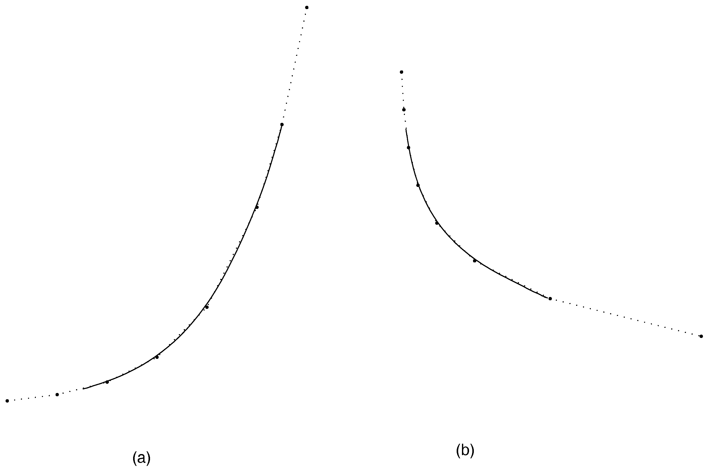
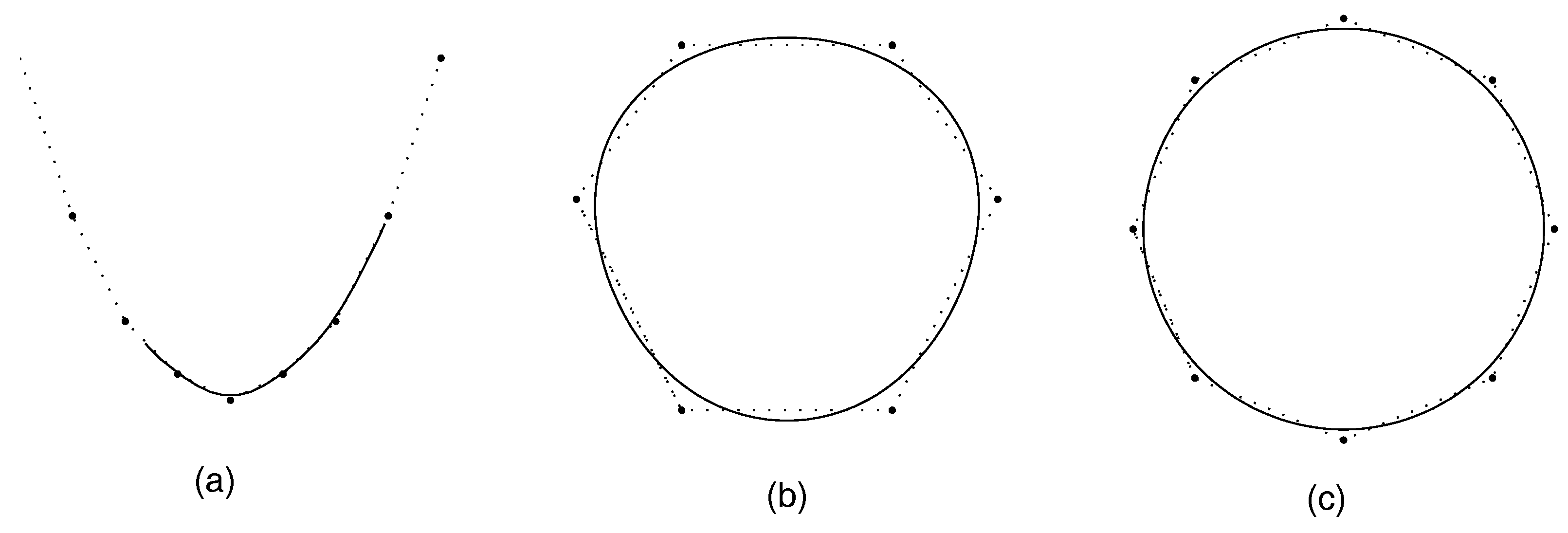
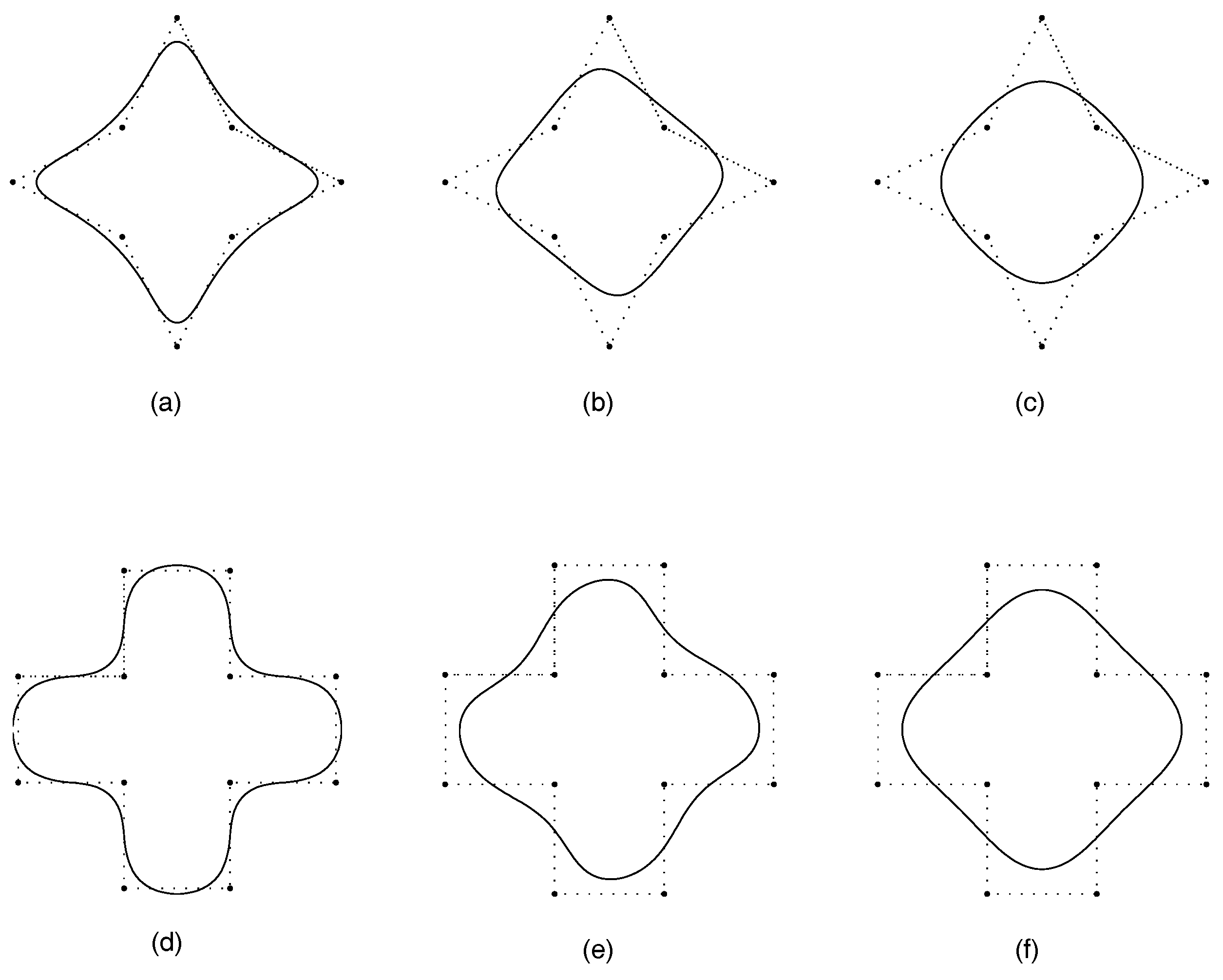
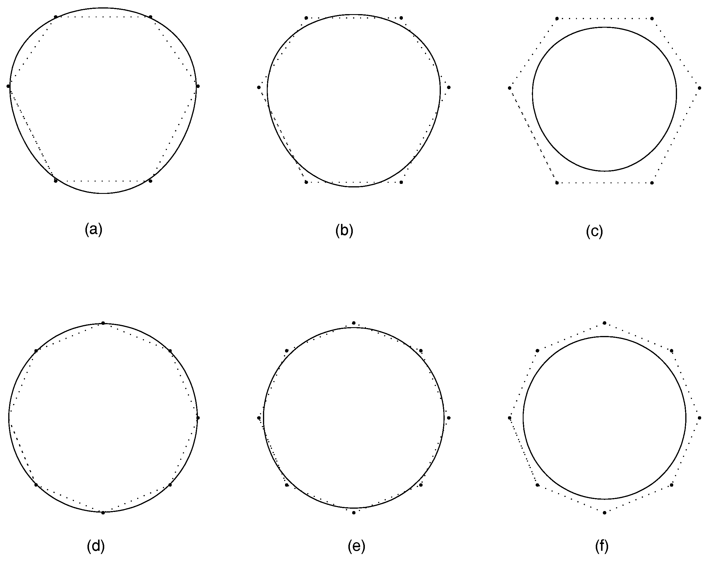
5. Conclusions and Numerical Examples

In this paper, we present a five-point subdivision scheme with two parameters and analyze the uniform convergence and $C^k$, the continuity of this scheme. When parameters u and v take the specific values, the five-point scheme reduces to a four-point scheme, which can generate $C^3$ limit curves. The shape-preserving properties of the four-point scheme are analyzed. In this section, a few examples are given to show the effect of the scheme (4), and to illustrate the efficiency and the shape-preserving effect of the scheme (5). Compared with the four-point scheme in [7] and the cubic uniform B-spline curves in [8], the curves generated by our scheme (5) have higher continuity and are closer to the control polygons.

In Figure 1, for given different initial control polygons, our subdivision scheme (4) generates different approximation effects, $C^3$ limit curves and $C^7$ limit curves.

In Figure 2, for given two initial control polygons which are strictly monotone increasing and strictly monotone decreasing respectively, the limit curves generated by the subdivision scheme (5) are monotone preserving.

In Figure 3, for given different initial control polygons, which are strictly convex, the limit curves generated by the subdivision scheme (5) are strictly convex. We can find that the curves generated by our scheme (5) are very close to the control polygons.

In Figure 4, for given different initial control polygons, compared with the four-point scheme in [7] and the cubic uniform B-spline curves in [8], the curves generated by our scheme (5) have higher continuity and are closer to the control polygons.

References

1. Dyn, N.; Levin, D.; Gregory, J.A. A 4-point interpolatory subdivision scheme for curve design. Comput. Aided Geom. Des. 1987, 4, 257–268. [Google Scholar] [CrossRef]
2. Dyn, N. Subdivision schemes in CAGD. In Advances in Numerical Analysis II: Wavelets, Subdivision Algorithms, and Radial Basis Functions; Light, W., Ed.; Oxford University Press: Oxford, UK, 1992; pp. 36–104. [Google Scholar]
3. Dyn, N.; Levin, D.; Micchelli, C.A. Using parameters to increase smoothness of curves and surfaces generated by subdivision. Comput. Aided Geom. Des. 1990, 7, 129–140. [Google Scholar] [CrossRef]
4. Dyn, N.; Kuijt, F.; Levin, D.; Damme, R.V. Convexity preservation of the four-point interpolatory subdivision scheme. Comput. Aided Geom. Des. 1999, 16, 789–792. [Google Scholar] [CrossRef]
5. Kuijt, F.; van Damme, R. Monotonicity preserving interpolatory subdivision schemes. J. Comput. Appl. Math. 1999, 101, 203–229. [Google Scholar] [CrossRef]
6. Kuijt, F.; van Damme, R. Shape preserving interpolatory subdivision schemes for nonuniform data. J. Approx. Theory 2002, 114, 1–32. [Google Scholar] [CrossRef]
7. Dyn, N.; Floater, M.S.; Hormann, K. A C2 four-point subdivision scheme with fourth order accuracy and its extensions. In Mathematical Methods for Curves and Surfaces: Tromsø 2004; Dahlen, M., Morken, K., Schumaker, L.L., Eds.; Nashboro Press: Brentwood, TN, USA, 2005; pp. 145–156. [Google Scholar]
8. Zheng, H.; Ye, Z.; Zhao, H. A class of four-point subdivision schemes with two parameters and its properties. J. Comput. Aided Des. Comput. Gr. 2004, 16, 1140–1145. (In Chinese) [Google Scholar]
9. Cai, Z. Convergence, error estimation and some properties of four-point interpolation subdivision scheme. Comput. Aided Geom. Des. 1995, 12, 459–468. [Google Scholar]
10. Cao, Y. The sufficient and necessary conditions of C2 continuity of the four-point interpolate subdivision scheme for curve and surface. J. Comput. Aided Des. Comput. Gr. 2003, 15, 961–966. (In Chinese) [Google Scholar]
11. Siddiqi, S.S.; Ahmad, N. A new five-point approximating subdivision scheme. Int. J. Comput. Math. 2008, 85, 65–72. [Google Scholar] [CrossRef]
12. Hao, Y.X.; Wang, R.H.; Li, C.J. Analysis of a 6-point binary subdivision scheme. Appl. Math. Comput. 2011, 218, 3209–3216. [Google Scholar] [CrossRef]
13. Cao, H.; Tan, J. A binary five-point relaxation subdivision scheme. J. Inf. Comput. Sci. 2013, 10, 5903–5910. [Google Scholar] [CrossRef]
14. Tan, J.; Yao, Y.; Cao, H.; Zhang, L. Convexity preservation of five-point binary subdivision scheme with a parameter. Appl. Math. Comput. 2014, 245, 279–288. [Google Scholar] [CrossRef]
15. Tan, J.; Tong, G.; Zhang, L.; Xie, J. Four point interpolatory-corner cutting subdivision. Appl. Math. Comput. 2015, 265, 819–825. [Google Scholar] [CrossRef]
16. Rehan, K.; Siddiqi, S.S. A combined binary 6-point subdivision scheme. Appl. Math. Comput. 2015, 270, 130–135. [Google Scholar] [CrossRef]
17. Conti, C.; Hormann, K. Polynomial reproduction for univariate subdivision schemes of any arity. J. Approx. Theory 2011, 163, 413–437. [Google Scholar] [CrossRef]
Figure 1. Our scheme (4) generates C 3 and C 7 limit curves. The initial control polygon is drawn by a dotted line, and the limit curve obtained by our scheme (4) is marked by a full line. (a,d) v = 0, u = 1, C 3 ; (b,e) v = 1/2, u = 1/2, C 3 ; (c,f) v = 1, u = 0, C 7 .
Mca 22 00022 g001
Figure 2. Our scheme (5) generates some monotone preserving C 3 limit curves; (a) increasing monotone, and (b) decreasing monotone. The initial control polygon is drawn by a dotted line, and the limit curve obtained by our scheme (5) is marked by a full line.
Mca 22 00022 g002
Figure 3. Our scheme (5) generates some strictly convex preserving C 3 limit curves (full line), given different (a–c) initial control polygons (dotted line).
Mca 22 00022 g003
Figure 4. Comparison of our scheme (5) ( C 3 limit curves) (b,e) with those proposed in [7] ( C 2 limit curves) (a,d) and [8] ( C 4 limit curves) (c,f). The initial control polygon is drawn by a dotted line, and the limit curve is marked by a full line.
Mca 22 00022 g004