New Scientific Contribution on the 2-D Subdomain Technique in Polar Coordinates: Taking into Account of Iron Parts


1
Département ENERGIE, FEMTO-ST, CNRS, University Bourgogne Franche-Comté, F90000 Belfort, France
2
Laboratoire de Rcherche en Electrotechnique (LRE-ENP), 16200 Algiers, Algeria
*
Author to whom correspondence should be addressed.
Math. Comput. Appl. 2017, 22(4), 42; https://doi.org/10.3390/mca22040042
Submission received: 22 July 2017
/
Revised: 21 October 2017
/
Accepted: 23 October 2017
/
Published: 25 October 2017
Abstract
:This paper presents a new scientific contribution to the two-dimensional red(2-D) subdomain technique in polar coordinates taking into account the finite relative permeability of the ferromagnetic material. The constant relative permeability corresponds to the linear part of the nonlinear curve. As in the conventional technique, the separation of variables method and the Fourier series are used for the resolution of magnetostatic Maxwell equations in each region. The general solutions of the magnetic field in subdomains, as well as the boundary conditions (BCs) between regions are different from the conventional method. In the proposed method, the magnetic field solution in each subdomain is a superposition of two magnetic quantities in the two directions (i.e., r- and -axis), and the BCs between two regions are also in both directions. For example, the scientific contribution has been applied to an air- or iron-cored coil supplied by a constant current. The distribution of local quantities (i.e., the magnetic vector potential and flux density) has been validated by a corresponding 2-D finite-element analysis (FEA). The obtained semi-analytical results are in very good agreement with those of the numerical method.
1. Introduction
The full calculation of the magnetic field in electrical engineering applications is the first step for their design and optimization. The methods of magnetic field prediction can be classified into various categories [1]:
Currently, the works on design are based on (semi-)analytical models (i.e., equivalent circuit, conformal transformation and Maxwell–Fourier methods). This type of model consists of a (non)linear system of N analytical equations solved analytically or numerically. In comparison with the other methods, under certain geometrical and physical assumptions, these models permit obtaining accurate analytical expressions of the magnetic field and are known as fast for the local/global electromagnetic performances prediction. At present, Maxwell–Fourier methods are one of the most used semi-analytic approaches with very accurate results (i.e., error less than 5%) on the electromagnetic performances calculation. These models are based on the formal resolution of Maxwell’s equations in Cartesian, cylindrical or spherical coordinates by using the separation of variables method and the Fourier’s series. Taking into account iron parts and/or the effect of local/global saturation is still a scientific challenge in Maxwell–Fourier methods, which is rarely explored in the literature [16,17,18]. Recently, Dubas et al. (2017) [1] realized an overview of the existing (semi-)analytical models in Maxwell–Fourier methods with the effect of local/global saturation, which can thus be classified as follows:
The consideration of the effect of local/global saturation appears in hybrid models, where the solution is established analytically in concentric regions of very low permeability (e.g., air-gap and magnets), and other methods (e.g., numerical or magnetic equivalent circuit) are sought in regions where the saturation effect cannot be neglected. The other models (i.e., multi-layers models, TREE method and subdomain technique) are more focused on the global saturation. Some details and (dis)advantages of these techniques can be found in [1]. In most semi-analytical models based on the subdomain technique, the iron parts are considered to be infinite permeable due to the variation of material proprieties in the various directions, so that the saturation effect is neglected [16,17,18]. The first paper introducing the iron parts in the magnetic field calculation by using the subdomain technique is [1], where the authors solve partial differential equations (PDEs) of the magnetic potential vector in Cartesian coordinates in which the subdomains connection is performed directly in both directions (i.e., x- and y-edges). The 2-D magnetostatic model has been applied to an air- or iron-cored coil supplied by a constant current. In [33], the authors propose a 2-D semi-analytical model in spoke-type magnet synchronous machines based on the subdomain technique in polar coordinates with the Taylor polynomial of degree three by focusing on the consideration of iron. The iron magnetic permeability is supposed constant corresponding to the linear zone of the nonlinear B(H) curve. The subdomains’ connection is carried out in both directions (i.e., r- and -edges). The general solution of the magnetic field is obtained by using the traditional boundary condition (BCs), in addition to new radial BCs (e.g., between the magnets and the rotor teeth, between the teeth and the slots of the stator), which are traduced into a system of linear equations according to Taylor series expansion. In [34], this semi-analytical model has been extended taking into account the initial magnetization curve in each soft-magnetic subdomain by an iterative procedure.
In the literature, to the authors’ knowledge, there exists no exact 2-D subdomain technique in polar coordinates taking into account iron parts with(out) the nonlinear curve and not using the Taylor series expansion to satisfy the r-edges BCs. Thus, in this paper, the research work contributes to the continuous improvement of the 2-D subdomain technique. Moreover, it is an extension of [1] in polar coordinates . Section 2 presents this new scientific contribution. By applying the principle of superposition on the magnetic quantities in order to respect the BCs on the various edges, the general solution of the magnetic field is decomposed in Fourier’s series into two general solutions in both directions (i.e., r- and -edges). It allows the evaluation of the local distribution of flux densities in the iron parts with a global saturation, does not have numerical convergence problems contrary to others models and would easily introduce the current penetration effect in the conductive materials. The semi-analytical solution is exact as in [1] and does not use the Taylor polynomial to satisfy the r-edges BCs contrary to [33,34]. For example, it was applied to an air- or iron-cored coil supplied by a constant current. The iron magnetic permeability is constant corresponding to the linear zone of the nonlinear curve [1,33]. Nevertheless, as in [29,30,34], the saturation effect could be taken into account by an iterative calculation considering, at each iteration, a constant relative magnetic permeability according to the nonlinear curve. However, this is beyond the scope of the paper. In Section 3, in order to confirm the effectiveness of the proposed technique, all semi-analytical results are then compared to those found by 2-D finite-element analysis (FEA) [40]. The comparisons are very satisfying in amplitudes and waveforms.
2. A 2-D Subdomain Technique of the Magnetic Field in Polar Coordinates
2.1. Model Description and Assumptions
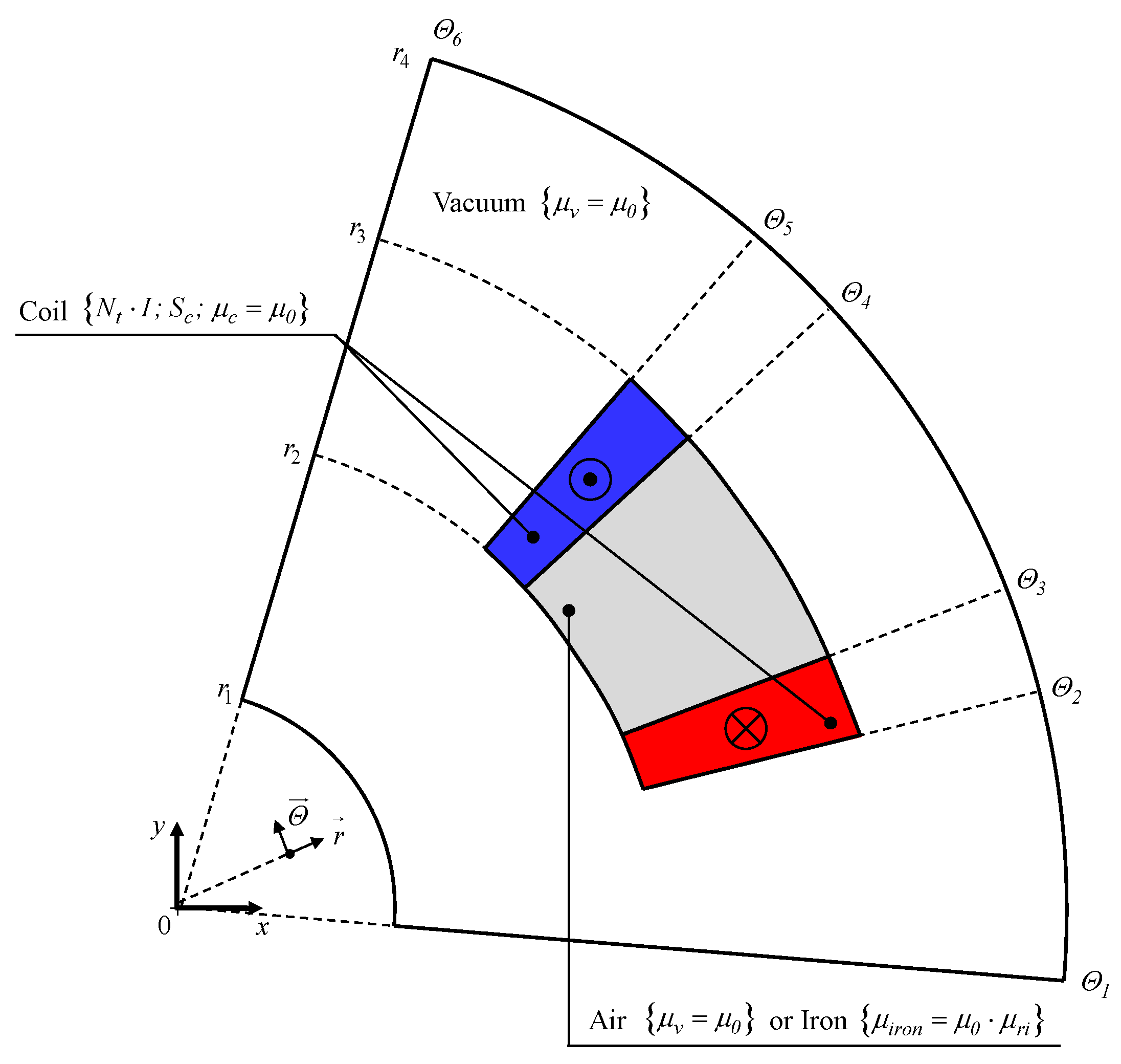
Figure 1 represents the physical and geometrical parameters of an air- or iron-cored coil with turns of copper wire supplied by a constant current I. The electromagnetic device is surrounded by an infinite box with a null value of magnetic vector potential at it boundaries.
The analytical prediction of the magnetic field based on the 2-D subdomain technique is done by solving magnetostatic Maxwell equations in polar coordinates with the following assumptions:
- The magnetic vector potential has only one component along the z-axis (i.e., ), and then, the end-effects are not considered;
- All materials are isotropic, and the permeabilities are supposed as constants in both directions (i.e., r- and -axis);
- All electrical conductivities of materials are supposed as nulls (i.e., the eddy-currents induced in the copper/iron are neglected).
2.2. Problem Discretization in Regions
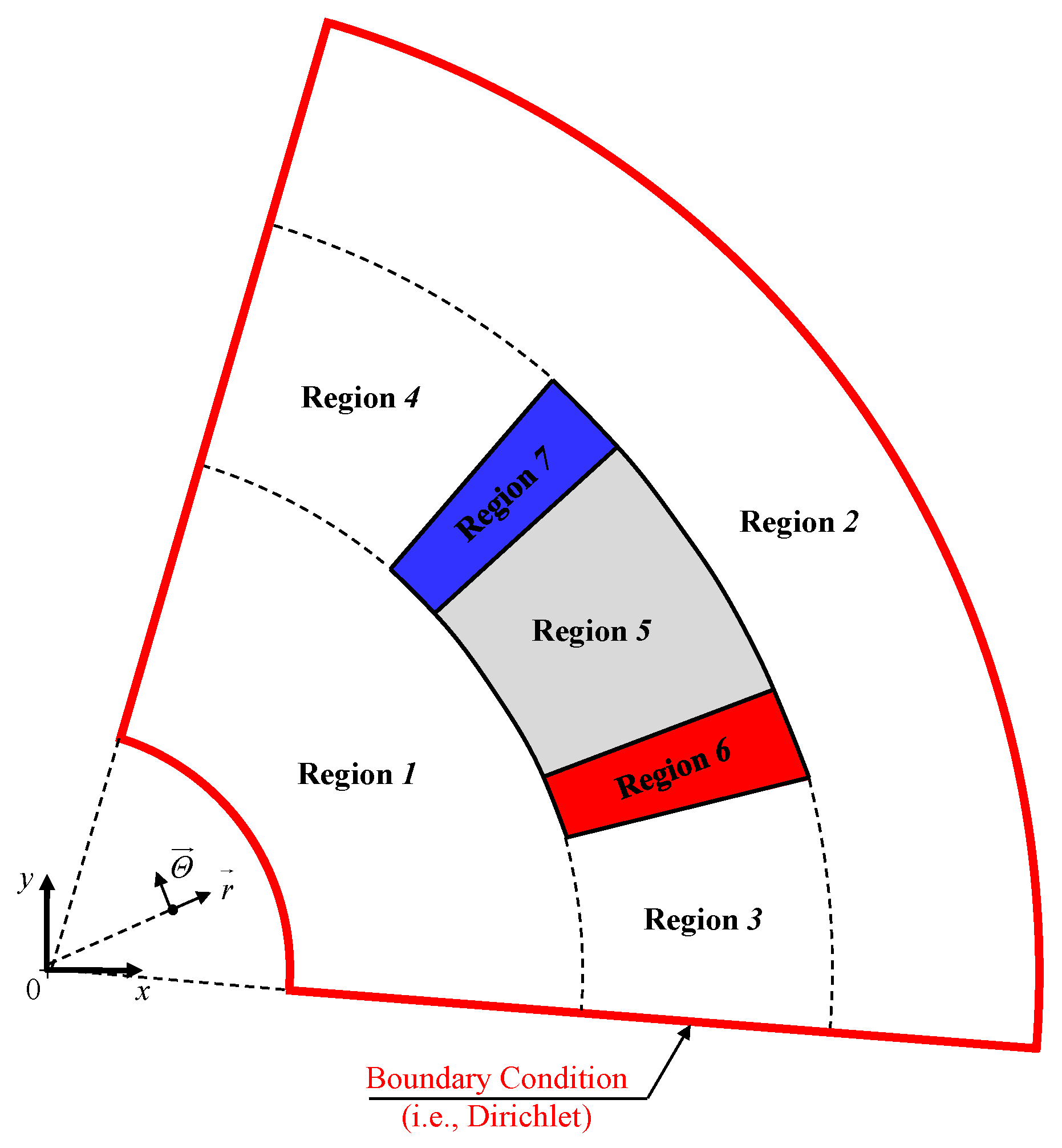
In Figure 2, we present the studied electromagnetic device, which is divided into seven regions with , viz.,
- Region 1 , with ;
- Region 2 , with ;
- Region 3 , with ;
- Region 4 , with ;
- Region 5 (i.e., the air or iron in the middle of the coil) , with for the air or for the iron;
- Region 6 (i.e., the forward conductor) , with ;
- Region 7 (i.e., the return conductor) , with .
2.3. Governing PDEs in Polar Coordinates: Laplace’s and Poisson’s Equations
According to Equation (A1) (see Appendix A), the distribution of the magnetic vector potential in polar coordinates is governed by:
where is the current density of the coil defined by:
in which is the conductor surface and (with and ) is the coefficient that represents the current direction in the conductor.
According to Appendix A, the resolution of Laplace’s and Poisson’s equations by using the separation of variables method and Fourier’s series permit obtaining two potentials in both directions, viz., for the -edges (in Equation (A2b)) and for the r-edges (in Equation (A2c)). The spatial frequency (or periodicity) of and is respectively defined by and with and the spatial harmonic orders.
2.4. Definition of Boundary Conditions
In electromagnetics, the general solutions of various regions depend on the BCs at the interface of two surfaces, which are defined by the continuity of the normal flux density and parallel field intensity [1]. On the outer BCs for and , satisfies the Dirichlet BC (see Figure 2), viz., .
Figure 3 represents the respective BCs at the interface between the various regions in both directions (i.e., r- and -edges).
2.5. General Solutions of Various Regions
2.5.1. Region 1
The solutions of , and are determined by Case-Study No. 1 (i.e., imposed on all edges of a region) in Appendix B. The BCs on the r-edges of the region (see Figure 3a) are met by posing in Equation (A11). Therefore, satisfying the BCs of Figure 3a and the solution of Equation (1a) is given by:
the components of by:
where and are defined in Equation (A9), the spatial harmonic orders in Region 1, the integration constant and with .
Using a Fourier series expansion of (see Figure 3a) over the interval , the integration constant is determined in Appendix C with:
2.5.2. Region 2
The same method as Region 1 is used to define the general solution in Region 2. By posing in Equation (A11) (see Appendix B), satisfying the BCs of Figure 3b and the solution of Equation (1a) is given by:
the components of by:
where is the spatial harmonic orders in Region 2, the integration constant and with .
Using a Fourier series expansion of (see Figure 3b) over the interval , the integration constant is determined in Appendix C with:
2.5.3. Region 3
The solutions of , and are determined by the Case-Study No. 1 (i.e., imposed on all edges of a region) in Appendix B. The BCs on the -edges of the region (see Figure 3c) are met by posing in Equations (A6)–(A8). Therefore, satisfying the BCs of Figure 3c and the solution of Equation (1a) is given by:
the r-component of by:
the -component of by:
where and are the spatial harmonic orders in Region 3; , and the integration constants; with ; and with .
Using Fourier series expansion of and (see Figure 3c) over the interval , the integration constants and are determined in Appendix C with:
With a weighting function and using a Fourier series expansion of (see Figure 3c) over the interval , the integration constant is determined in Appendix C with:
2.5.4. Region 4
The solution in Region 4 is obtained using the same development as Region 3. By posing in Equations (A6)–(A8) (see Appendix B), satisfying the BCs of Figure 3d and the solution of Equation (1a) is given by:
the r-component of by:
the -component of by:
where and are the spatial harmonic orders in Region 4; , and the integration constants; with ; and with .
Using Fourier series expansion of and (see Figure 3d) over the interval , the integration constants and are determined in Appendix B with:
With a weighting function and using a Fourier series expansion of (see Figure 3d) over the interval , the integration constant is determined in Appendix C with:
2.5.5. Region 5
For Region 5, the general solution is given according to the BCs of Case-Study No. 1 (i.e., imposed on all edges of a region) in Appendix B. Therefore, satisfying the BCs of Figure 3e and the solution of Equation (1a) is given by:
the r-component of by:
the -component of by:
where and are the spatial harmonic orders in Region 5; , , and the integration constants; with ; and with .
Using Fourier series expansion of and (see Figure 3e) over the interval , the integration constants and are determined in Appendix C with:
With a weighting function and using a Fourier series expansion of and (see Figure 3e) over the interval , the integration constants and are determined in Appendix C with:
2.5.6. Region 6
For Region 6, the general solution is given according to the BCs of Case-Study No. 2 (i.e., and are respectively imposed on r- and -edges of a region) in Appendix B. Therefore, satisfying the BCs of Figure 3f and the solution of Equation (1b) is given by:
Considering Equations (26b) and (26c), as well as the form of the current density distribution, i.e., Equation (2), a particular solution can be found. The following particular solution is proposed:
The r-component of is defined by:
and the -component of by:
where and are the spatial harmonic orders in Region 6; , , , , and the integration constants; with ; and with .
Using Fourier series expansion of and (see Figure 3f) over the interval , the integration constants and and and are determined in Appendix C with:
Using a Fourier series expansion of and (see Figure 3f) over the interval , the integration constants and are determined in Appendix C with:
2.5.7. Region 7
The solution in Region 7 is using the same development as Region 6. Thus, satisfying the BCs of Figure 3g and the solution of Equation (2) is defined by:
The r-component of is defined by:
and the -component of by:
where and are the spatial harmonic orders in Region 7; , , , , and the integration constants; with ; and with .
Using Fourier series expansion of and (see Figure 3g) over the interval , the integration constants and and and are determined in Appendix C with:
Using a Fourier series expansion of and (see Figure 3g) over the interval , the integration constants and are determined in Appendix C with:
3. Validation of the Semi-Analytic Method with Finite-Element Analysis
3.1. Introduction
The objective of this section is to validate the 2-D subdomain technique in polar coordinates on the magnetic field distribution in relation to the numerical method. The physical and geometrical parameters of studied electromagnetic device are given in Table 1.
For this validation, the air- or iron-cored coil has been modeled using Cedrat’s Flux2D (Version 10.2.1, Altair Engineering, Meylan Cedex, France) software package (i.e., an advanced finite-element method-based numeric field analysis program) [40]. FEA is done with the same assumptions as the semi-analytical model (see Section 2.1). The linear system is given in Appendix C and has been implemented in MATLAB® (R2015a, MathWorks, Natick, MA, USA) by using the sparse matrix/vectors. A discussion of the numerical problems (viz., harmonics and ill-conditioned systems) of such semi-analytical models has been clarified in [1]. The Maxwell–Fourier methods exhibit a similar problem to the numerical methods due to the periodicity of Fourier series and, consequently, to the finite number of harmonics. Hence, and in the various regions (see Section 2.5) have been computed with a finite number of spatial harmonics terms – (for the -edges) and – (for the r-edges). As indicated in [41,42], these spatial harmonics terms, given in Table 1, have been imposed according to an optimal ratio, i.e., for given,
The linear system size depends on the number of: (i) regions; (ii) BCs; and (iii) harmonics of each subdomain. In our study, the linear system named Equation (A17) consists of 2036 elements, which is much smaller than the 2-D FEA mesh having 3,081 surfaces elements of second order (viz., the triangles number of system) with the number of excellent quality elements equal to 100%. For information, the 2-D FEA mesh for an air- or iron-cored coil is illustrated in Figure 4. The personal computer used for this comparison has the following characteristics: HP Z800 Intel(R) Xeon(R) CPU @ 2.4 GHz (with two processors) RAM 16 Go 64 bits. The computation time of 2-D subdomain model is divided by two (viz., 0.5 s for 2-D subdomain model and 1 s for the 2-D FEA).
3.2. Results Discussion
The validation paths of and for the semi-analytic and numeric comparison are given in Figure 5.
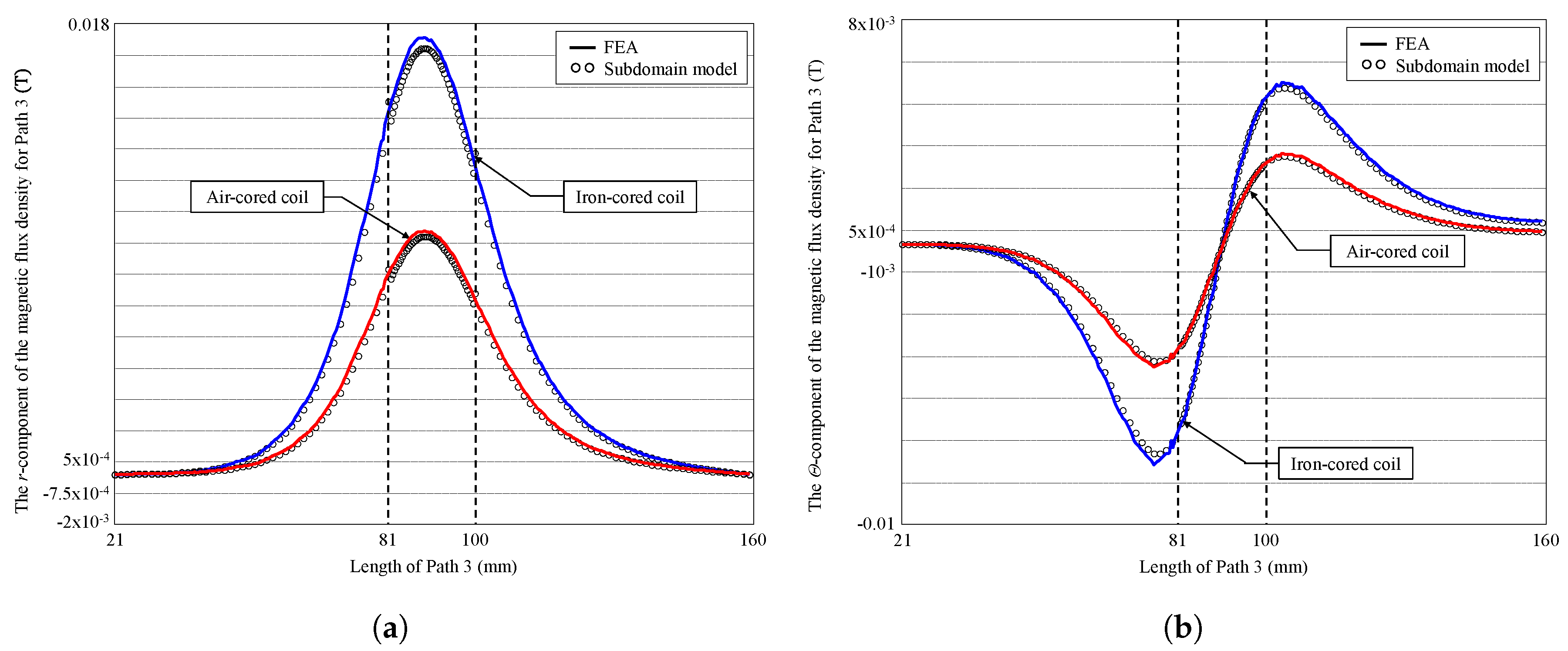
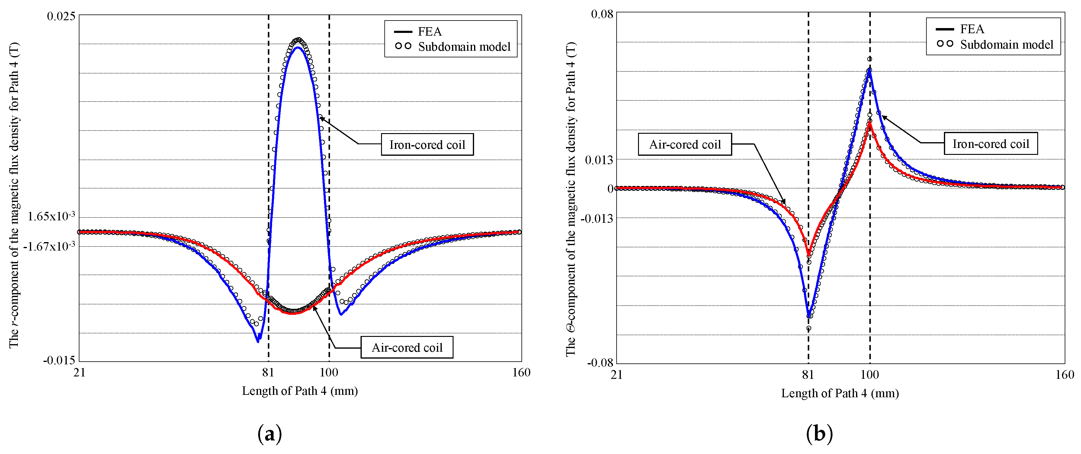
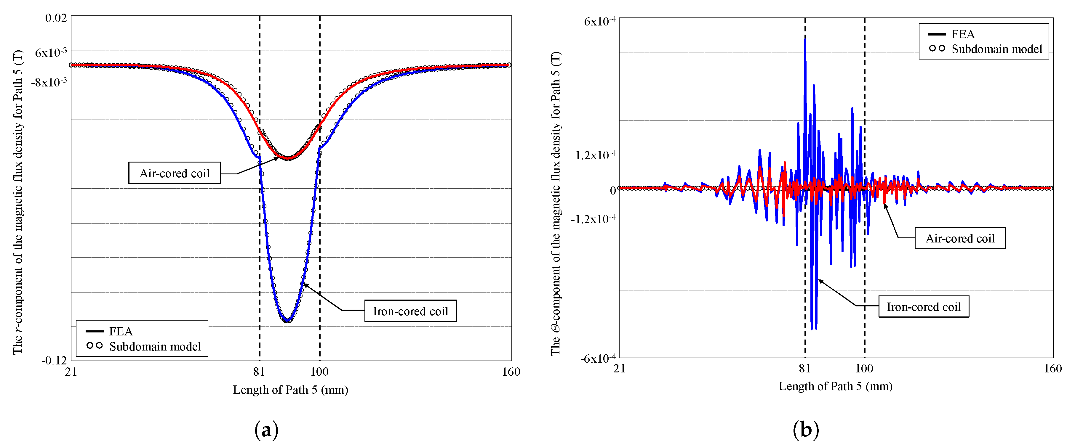
The waveforms of global quantities are shown on different paths in Figure 6 for and in Figure 7, Figure 8, Figure 9, Figure 10 and Figure 11 for the components of . The solid lines represent the global quantities computed by the 2-D FEA, and the circles correspond to the 2-D subdomain model. Comparing those results with 2-D FEA, it can be shown that a very good evaluation is obtained for and for the components of , whatever the paths, for both the air- and iron-core. This confirms that the effect of global saturation can be taken into account accurately. According to the concept of symmetry, it can be seen that in polar coordinates, there is only one symmetry of on Path 5 (viz., and in Figure 11) unlike the same electromagnetic device in Cartesian coordinates. Indeed, in Cartesian coordinates, there exist two symmetry axes of on Path 2 and Path 5 [1]. In polar coordinates, Path 2 does not correspond to a symmetry axis of ; consequently, and in Figure 8. It will be noted that the r-component of in Region 5 is more intense with the magnetic core (see Figure 8a) and that the magnetic leakages in the middle of the device in the -axis are equivalent for an air- and iron-cored coil (see Figure 8b). It is interesting to note that numerical peaks appear in the FEA results (see Figure 6e, Figure 7, Figure 8b and Figure 11b), which are mainly due to the mesh. The relative error is less than 1.5% for the various global quantities (see Figure 6a,c for the maximum error).
4. Conclusions
It has been demonstrated that there exists no exact semi-analytical model based on the 2-D subdomain technique in polar coordinates taking into account iron parts with(out) the nonlinear curve. An improved 2-D subdomain method in polar coordinates to study the magnetic field distribution in the iron parts with a finite relative permeability has been presented in this paper. Nevertheless, the research work is an extension of [1] in polar coordinates .
The proposed new subdomain model is applied to an air- or iron-cored coil supplied by a constant current. The magnetic field solutions in the subdomains and the BCs between regions are carried out in the two directions (i.e., r- and -axis). The iron relative permeability used in this model is constant and corresponds to the linear part of the nonlinear curve. However, the whole curve of the magnetic material can be applied with an iterative algorithm as in [29,30,34]. The proposed subdomain method in polar coordinates takes less computing time than the FEA (approximately two-fold versus to FEA). It is very suitable for the design and optimization of the electromechanical systems in general and electrical machines in particular. The semi-analytical results have been validated with FEA, and good agreement has been obtained in both amplitudes and waveforms.
The major scientific contribution could be applied to rotating electrical machines (e.g., radial-flux machines) in polar coordinates with(out) magnets supplied by a direct or alternate current (with any waveforms). Moreover, one advantage of this technique would be their exploitation in three-dimensional studies in order to reduce the computation time, which remains a major problem in this numerical method.
Author Contributions
The work presented here was carried out in cooperation among all authors, which have written the paper and have gave advice for the manuscripts.
Conflicts of Interest
The authors declare no conflict of interest.
Appendix A. The 2-D General Solution of PDEs (i.e., Laplace’s and Poisson’s Equations) in Polar Coordinates
Using the magnetostatic Maxwell’s equations (viz., the Maxwell–Ampere law, the Maxwell– Thomson law and the magnetic material equation) [1], the general PDEs in terms of magnetic vector potential with can be expressed in polar coordinates by:
where is the current density (due to supply currents) vector, is the magnetization vector (with for the vacuum/iron or for the magnets according to the magnetization direction [43]) and is the absolute magnetic permeability of the magnetic material in which and are respectively the vacuum permeability and the relative permeability of the magnetic material (with for the vacuum or for the magnets/iron).
The magnetic vector potential is governed by Poisson’s equation (i.e., ) or Laplace’s equation (i.e., ). Using the separation of variables method, the 2-D general solution of in both directions (i.e., r- and -edges) can be written as Fourier’s series:
where is the particular solution of respecting the second member in Equation (A1), – and – the integration constants, and the spatial frequency (or periodicity) of and and h and n the spatial harmonic orders.
Using , the components of magnetic flux density can be deduced by:
which leads to:
and:
Appendix B. Simplification of Laplace’s Equations According to Imposed BCs
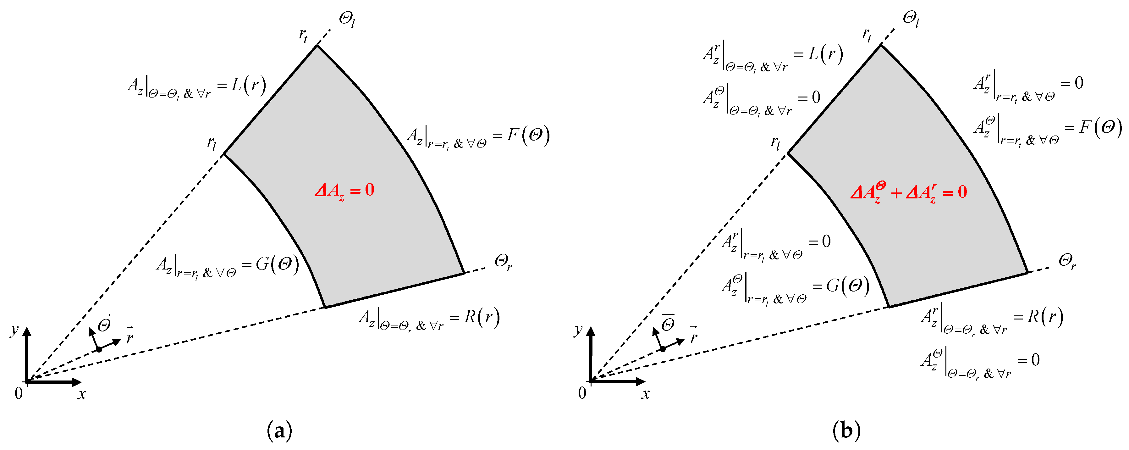
Appendix B.1. Case-Study No. 1: Imposed on all Edges of a Region
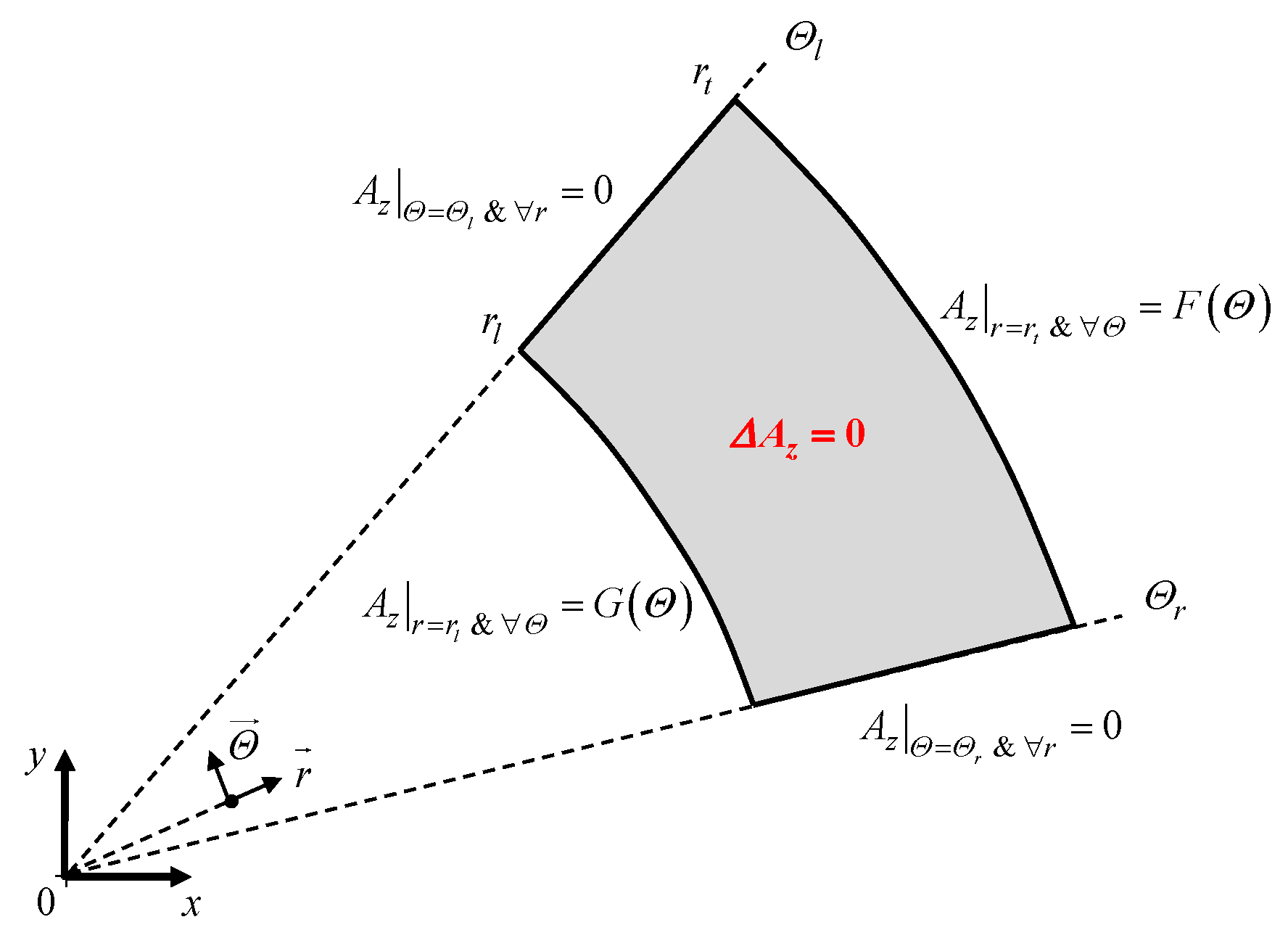
Figure A1a shows a region (for and ) whose is imposed on all edges. By respecting the BCs and applying the principle of superposition on the magnetic quantities, Figure A1a is redefined by Figure A1b.
Figure A1.
imposed on all edges of a region: (a) general and (b) principle of superposition.

In Case-Study No. 1, , i.e., Equation (A2), is redefined by:
the component of , i.e., Equation (A4), by:
and the component of , i.e., Equation (A5), by:
where , , and are new integration constants; with ; with ; and and are [44]:
with:
When on -edges and imposed on r-edges (see Figure A2), with in Equation (A6) is expressed by:
the r-component of with in Equation (A7) by:
the -component of with in Equation (A8) by:
Figure A2.
Particular case: on -edges and imposed on r-edges of a region.
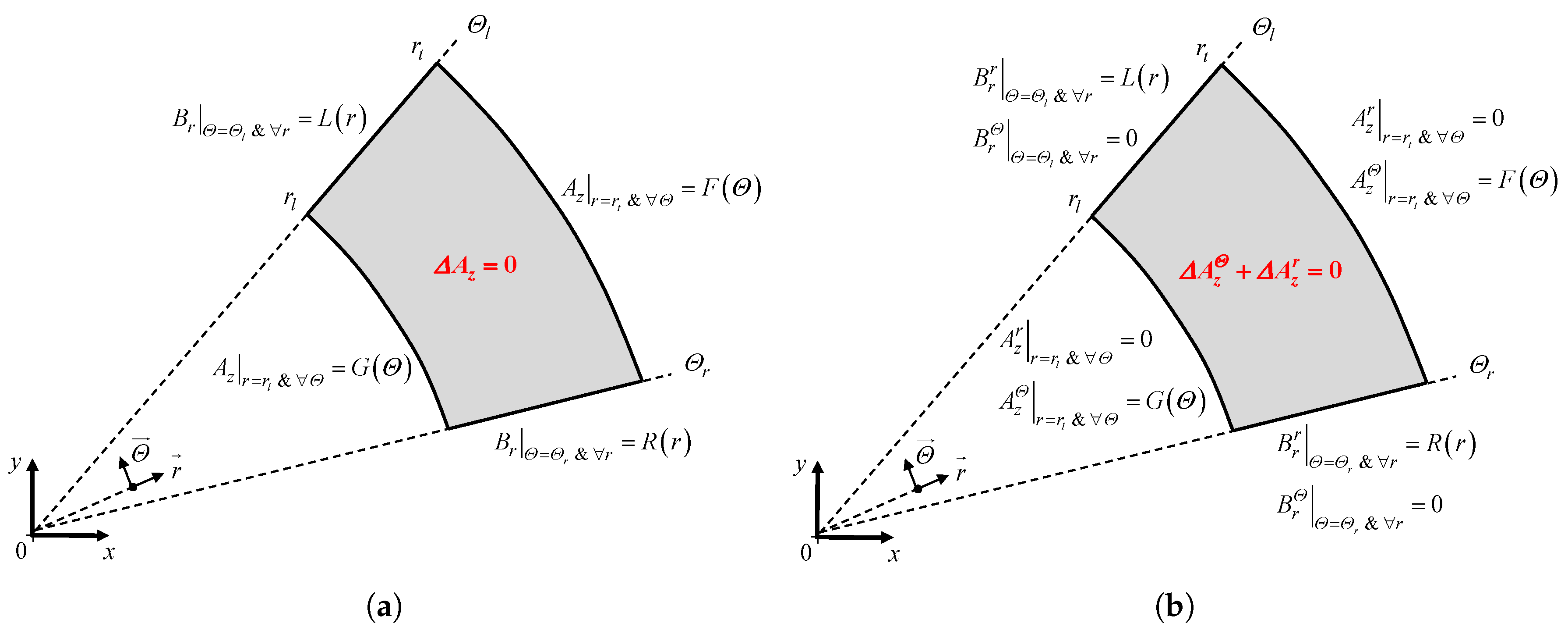
Appendix B.2. Case-Study No. 2: and Are Respectively Imposed on r- and Θ-Edges of a Region
Figure A3a shows a region (for and ) whose and are respectively imposed on r- and -edges. By respecting the BCs and applying the principle of superposition on the magnetic quantities, Figure A3a is redefined by Figure A3b.
Figure A3.
imposed on r-edges and imposed on -edges of a region: (a) general and (b) principle of superposition.
Figure A3.
imposed on r-edges and imposed on -edges of a region: (a) general and (b) principle of superposition.

In Case-Study No. 2, , i.e., Equation (A2), is redefined by:
the component of , i.e., Equation (A4), by:
and the component of , i.e., Equation (A5), by:
where , , , , and are new integration constants.
Appendix C. Solving of the Linear System
Appendix C.1. Calculation of General Integrals
For the determination of Fourier’s series coefficients, it is required to calculate general integrals of the form:
Appendix C.2. Determination of Integral Constants
The integration constants are determined by solving:
which consists of:
equations and unknowns [1], where − (for the -edges) and − (for the r-edges) are the maximal number of spatial harmonics in the various regions for the computation of and . To solve Equation (A17), a numerical matrix inversion is required for the calculation of . This set is implemented in MATLAB® (R2015a, MathWorks, Natick, MA, USA) by using the sparse matrix/vectors [1]. Usually, the two reasons for the possibility of including a finite number of harmonics is a limiting computational time and numerical accuracy [45].
The integration constants vector (of dimension ) is defined by:
The structure of the electromagnetic sources vector (of dimension ), as well as the BCs matrix (of dimension ) is given in [1] (see Section 2.6).The novel corresponding elements in and are defined as follows for Region 1:
for Region 2:
for Region 3:
for Region 4:
for Region 5:
for Region 6:
for Region 7:
References
- Dubas, F.; Boughrara, K. New scientific contribution on the 2-D subdomain technique in Cartesian coordinates: Taking into account of iron parts. Math. Comput. Appl. 2017, 22. [Google Scholar] [CrossRef]
- Lehmann, T. Méthode graphique pour déterminer le trajet des lignes de force dans l’air. Revue d’Électricité: La Lumière Électrique 1909, 43–45, 103–110, 137–142, 163–168. [Google Scholar]
- Jin, J. The Finite Element Method in Electromagnetic, 2nd ed.; John Wiley and Sons, Inc.: New York, NY, USA, 2002. [Google Scholar]
- Smith, G.D. Numerical Solution of Partial Differential Equations: Finite Difference Methods, 3rd ed.; Clarendon Press: Oxford, UK, 1985. [Google Scholar]
- Wrobel, L.C.; Aliabadi, M.H. The Boundary Element Method; John Wiley and Sons, Inc.: New York, NY, USA, 2002. [Google Scholar]
- Kron, G. Equivalent Circuits of Electric Machinery; John Wiley and Sons, Inc.: New York, NY, USA; Chapman and Hall, Ltd.: London, UK, 1951. [Google Scholar]
- Holman, J.P. Heat Transfer, 6th ed.; McGraw-Hill Book Compagny: New York, NY, USA, 1986. [Google Scholar]
- Roters, H.C. Electromagnetic Devices; John Wiley and Sons, Inc.: New York, NY, USA, 1941. [Google Scholar]
- Driscoll, T.A.; Trefethen, L.N. Schwarz-Christoffel Mapping; Cambridge University Press: Cambridge, UK, 2002. [Google Scholar]
- Hague, B. Electromagnetic Problems in Electrical Engineering; Oxford University Press: London, UK, 1929. [Google Scholar]
- Sylvester, P. Modern Electromagnetic Fields; Prentice-Hall: London, UK, 1968. [Google Scholar]
- Stoll, R.L. The Analysis of Eddy Currents; Clarendon Press: Oxford, UK, 1974. [Google Scholar]
- Binns, K.J.; Lawrenson, P.J.; Trowbridge, C.W. The Analytical and Numerical Solution of Electric and Magnetic Fields; John Wiley and Sons, Inc.: New York, NY, USA, 1992. [Google Scholar]
- Melcher, J.R. Continuum Electromechanics; MIT Press: Cambridge, MA, USA, 1981. [Google Scholar]
- Farlow, S.J. Partial Differential Equations for Scientists and Engineers; Dover, Inc.: New York, NY, USA, 1993. [Google Scholar]
- Dubas, F.; Espanet, C. Analytical solution of the magnetic field in permanent-magnet motors taking into account slotting effect: No-load vector potential and flux density calculation. IEEE Trans. Magn. 2009, 45, 2097–2109. [Google Scholar] [CrossRef]
- Tiegna, H.; Amara, Y.; Barakat, G. Overview of analytical models of permanent magnet electrical machines for analysis and design purposes. Math. Comput. Simul. 2013, 90, 162–177. [Google Scholar] [CrossRef]
- Devillers, E.; Le Besnerais, J.; Lubin, T.; Hecquet, M.; Lecointe, J.P. A review of subdomain modeling techniques in electrical machines: Performances and applications. In Proceedings of the XXII International Conference on Electrical Machines (ICEM), Lausanne, Switzerland, 4–7 September 2016. [Google Scholar]
- Kumar, P.; Bauer, P. Improved analytical model of a permanent-magnet brushless DC motor. IEEE Trans. Magn. 2008, 44, 2299–2309. [Google Scholar] [CrossRef]
- Dalal, A.; Kumar, P. Analytical model for permanent magnet motor with slotting effect, armature reaction, and ferromagnetic material property. IEEE Trans. Magn. 2015, 51. [Google Scholar] [CrossRef]
- Boules, N. Two-dimensional field analysis of cylindrical machines with permanent magnet excitation. IEEE Trans. Ind. Appl. 1984, IA-20, 1267–1277. [Google Scholar] [CrossRef]
- Berkani, M.S.; Sough, M.L.; Giurgea, S.; Dubas, F.; Boualem, B.; Espanet, C. A simple analytical approach to model saturation in surface mounted permanent magnet synchronous motors. In Proceedings of the 2015 IEEE Energy Conversion Congress and Exposition (ECCE), Montreal, QC, Canada, 20–24 September 2015. [Google Scholar]
- Mishkin, E. Theory of the squirrel-cage induction machine derived directly from Maxwell’s field equations. Q. J. Mech. Appl. Math. 1954, 7, 472–487. [Google Scholar] [CrossRef]
- Panaitescu, A.; Panaitescu, I. A field model for induction machines. In Proceedings of the International Conference on Electrical Machines (ICEM), Vigo, Spain, 10–12 September 1996. [Google Scholar]
- Madescu, G.; Boldea, I.; Miller, T.J.E. An analytical iterative model (AIM) for induction motor design. In Proceedings of the Conference Record of the I996 IEEE Industry Applications Conference Thirty-First IAS Annual Meeting, San Diego, CA, USA, 6–10 October 1996. [Google Scholar]
- Sprangers, R.L.J.; Motoasca, T.E.; Lomonova, E.A. Extended anisotropic layer theory for electrical machines. IEEE Trans. Magn. 2013, 49, 2217–2220. [Google Scholar] [CrossRef]
- Sprangers, R.L.J.; Paulides, J.J.H.; Gysen, B.L.J.; Lomonova, E.A. Magnetic saturation in semi-analytical harmonic modeling for electric machine analysis. IEEE Trans. Magn. 2016, 52. [Google Scholar] [CrossRef]
- Sprangers, R.L.J.; Paulides, J.J.H.; Gysen, B.L.J.; Waarma, J.; Lomonova, E.A. Semi-analytical framework for synchronous reluctance motor analysis including finite soft-magnetic material permeability. IEEE Trans. Magn. 2015, 51. [Google Scholar] [CrossRef]
- Djelloul, K.Z.; Boughrara, K.; Ibtiouen, R.; Dubas, F. Nonlinear analytical calculation of magnetic field and torque of switched reluctance machines. In Proceedings of the CISTEM, Marrakech-Benguérir, Maroc, 26–28 October 2016. [Google Scholar]
- Djelloul, K.Z.; Boughrara, K.; Dubas, F.; Ibtiouen, R. Nonlinear analytical prediction of magnetic field and electromagnétic performances in switched reluctance machines. IEEE Trans. Magn. 2017, 53. [Google Scholar] [CrossRef]
- Theodoulidis, T.P. Model of ferrite-cored probes for eddy current nondestructive evaluation. J. Appl. Phys. 2003, 93, 3071–3078. [Google Scholar] [CrossRef]
- Theodoulidis, T.P.; Bowler, J. Eddy-current interaction of a long coil with a slot in a conductive plate. IEEE Trans. Magn. 2005, 41, 1238–1247. [Google Scholar] [CrossRef]
- Roubache, L.; Boughrara, K.; Dubas, F.; Ibtiouen, R. Semi-Analytical modeling of spoke-type permanent-magnet machines considering the iron core relative permeability: Subdomain technique and Taylor polynomial. Prog. Electromagn. Res. B 2017, 77, 85–101. [Google Scholar] [CrossRef]
- Roubache, L.; Boughrara, K.; Dubas, F.; Ibtiouen, R. Semi-analytical modeling of spoke-type permanent-magnet machines considering nonlinear magnetic saturation: Subdomain Technique and Taylor polynomial. Math. Comput. Simul. 2017. Under review. [Google Scholar]
- Abdel-Razek, A.A.; Coulomb, J.L.; Feliachi, M.; Sabonnadière, J.C. The calculation of electromagnetic torque in saturated electric machines within combined numerical and analytical solutions of the field equations. IEEE Trans. Magn. 1981, 17, 3250–3252. [Google Scholar] [CrossRef]
- Liu, Z.J.; Bi, C.; Tan, H.C.; Low, T.S. A combined numerical and analytical approach for magnetic field analysis of permanent magnet machines. IEEE Trans. Magn. 1995, 31, 1372–1375. [Google Scholar] [CrossRef]
- Mirzayee, M.; Mehrjerdi, H.; Tsurkerman, I. Analysis of a high-speed solid rotor induction motor using coupled analytical method and reluctance networks. In Proceedings of the 2005 IEEE/ACES International Conference on Wireless Communications and Applied Computational Electromagnetics (ACES), Honolulu, HI, USA, 3–7 April 2005. [Google Scholar]
- Hemeida, A.; Sergeant, P. Analytical modeling of surface PMSM using a combined solution of Maxwell’s equations and magnetic equivalent circuit. IEEE Trans. Magn. 2014, 50. [Google Scholar] [CrossRef]
- Pluk, K.J.W.; Jansen, J.W.; Lomonova, E.A. 3-D hybrid analytical modeling: 3-D Fourier modeling combined with mesh-based 3-D magnetic equivalent circuits. IEEE Trans. Magn. 2015, 51. [Google Scholar] [CrossRef]
- Flux2D. General Operating Instructions, Version 10.2.1; Cedrat S.A. Electrical Engineering: Grenoble, France, 2008.
- Lee, S.W.; Jones, W.; Campbell, J. Convergence of numerical solution of iris-type discontinuity problems. IEEE Trans. Microw. Theory Tech. 1971, 19, 528–536. [Google Scholar]
- Mittra, R.; Itoh, T.; Li, T.-S. Analytical and numerical studies of the relative convergence phenomenon arising in the solution of an integral equation by the moment method. IEEE Trans. Microw. Theory Tech. 1972, 20, 96–104. [Google Scholar] [CrossRef]
- Rahideh, A.; Korakianitis, T. Analytical calculation of open-circuit magnetic field distribution of slotless brushless PM machines. Electr. Power Energy Syst. 2012, 44, 99–114. [Google Scholar] [CrossRef]
- Dubas, F.; Rahideh, A. Two-dimensional analytical PM eddy-current loss calculations in slotless PMSM equipped with surface-inset magnets. IEEE Trans. Magn. 2014, 50. [Google Scholar] [CrossRef]
- Gysen, B.L.J.; Meessen, K.J.; Paulides, J.J.H.; Lomonova, E.A. General formulation of the electromagnetic field distribution in machines and devices using Fourier analysis. IEEE Trans. Magn. 2010, 46, 39–52. [Google Scholar] [CrossRef]
Figure 1.
Physical and geometrical parameters (see Table 1) of air- or iron-cored coil where ⊗ and ⊙ are respectively the forward and return conductor. The variables are: the number of turns; I the supply current; the conductor surface; the vacuum magnetic permeability; the copper magnetic permeability; and the iron magnetic permeability.

Figure 2.
Definition of regions in the air- or iron-cored coil.

Figure 3.
Boundary Conditions (BCs) in both directions (i.e., r- and -edges): (a) Region 1; (b) Region 2; (c) Region 3; (d) Region 4; (e) Region 5; (f) Region 6; and (g) Region 7.
Figure 3.
Boundary Conditions (BCs) in both directions (i.e., r- and -edges): (a) Region 1; (b) Region 2; (c) Region 3; (d) Region 4; (e) Region 5; (f) Region 6; and (g) Region 7.
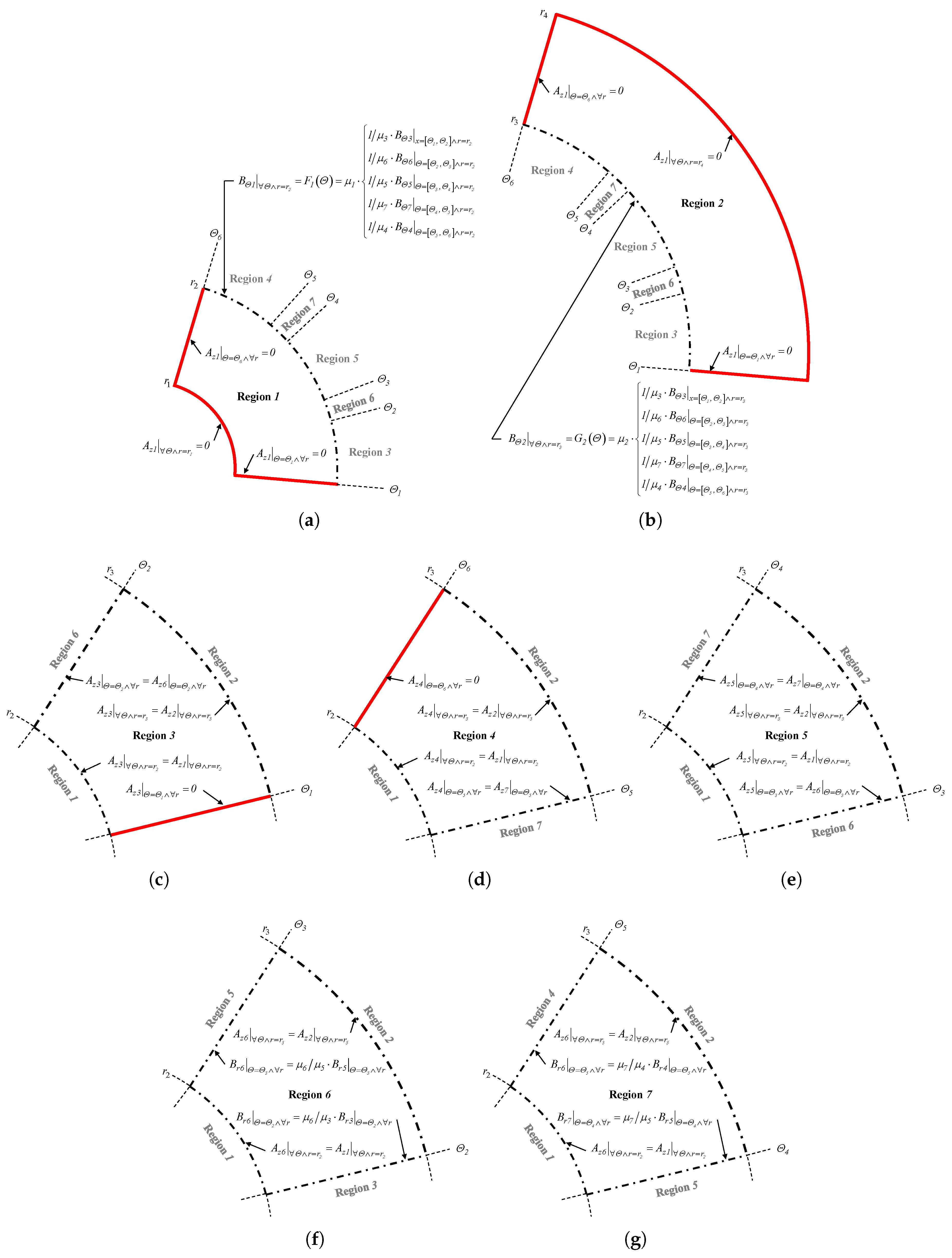
Figure 4.
2-D Finite-Element Analysis (FEA) mesh for the air- or iron-cored coil.
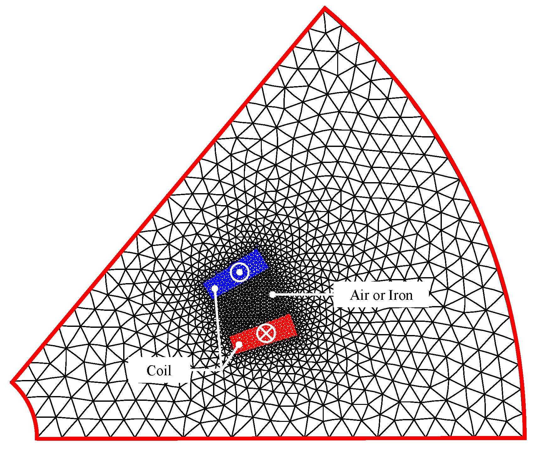
Figure 5.
Validation paths for the semi-analytic and numeric comparison.
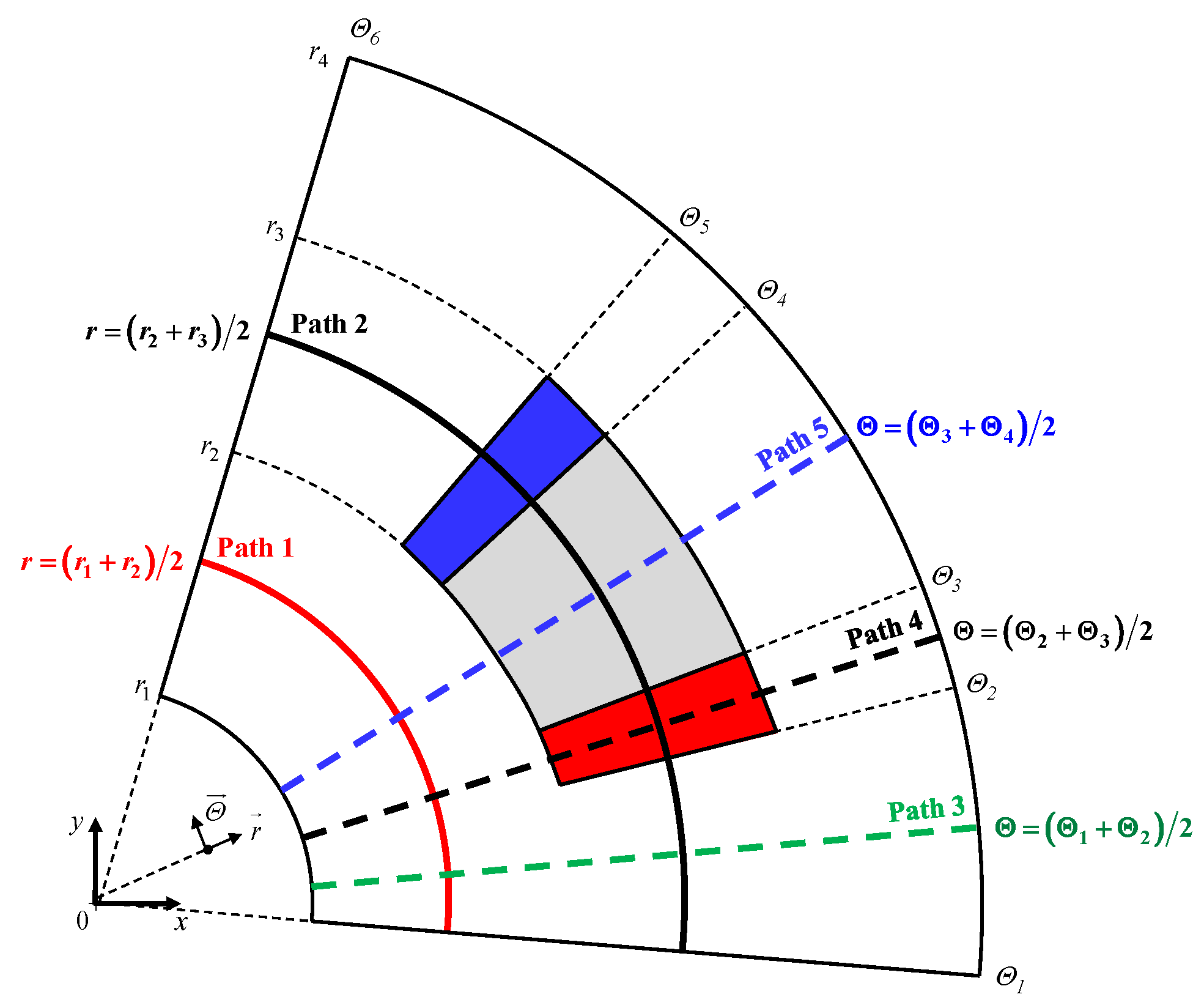
Figure 6.
Waveforms of for: (a) Path 1; (b) Path 2; (c) Path 3; (d) Path 4; and (e) Path 5.
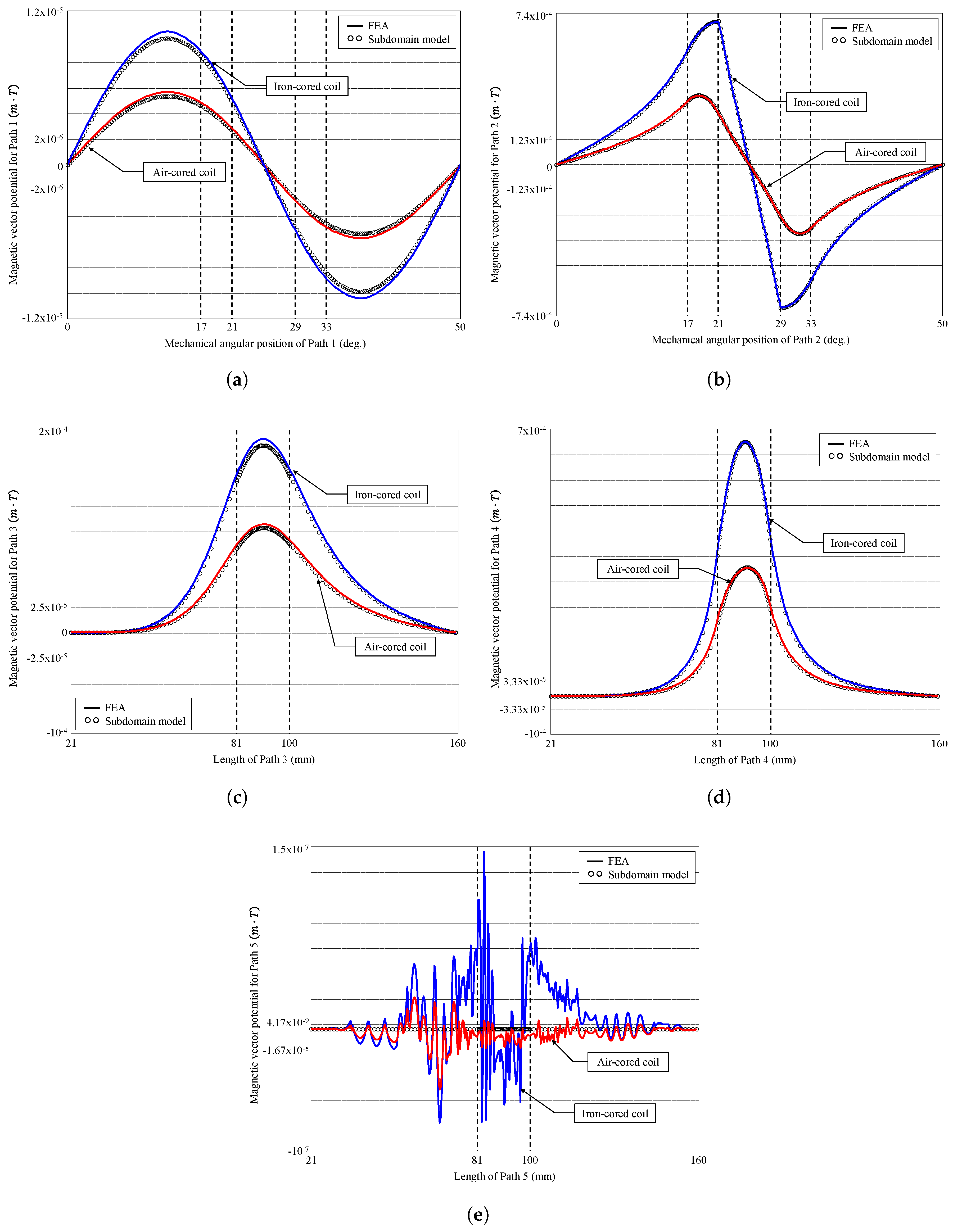
Figure 7.
Waveforms of for Path 1: (a) r- and (b) -component.
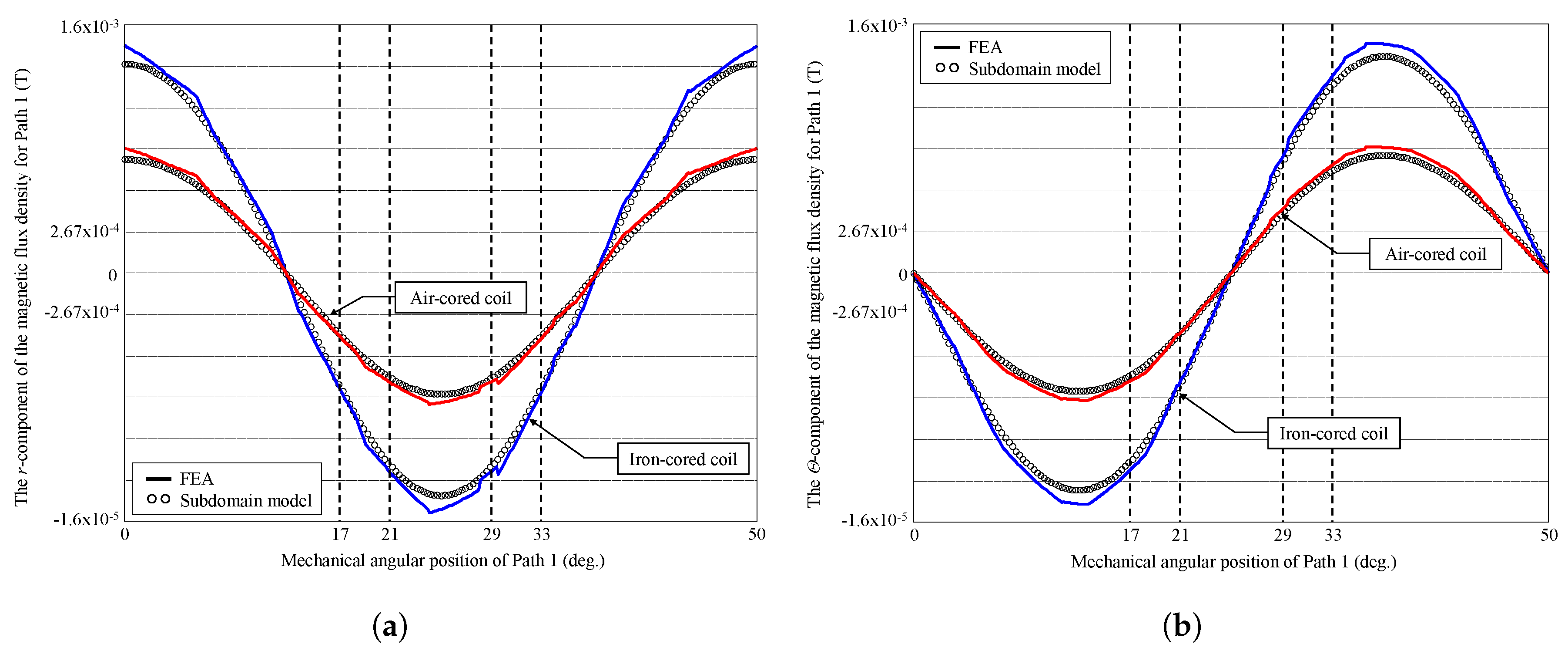
Figure 8.
Waveforms of for Path 2: (a) r- and (b) -component.
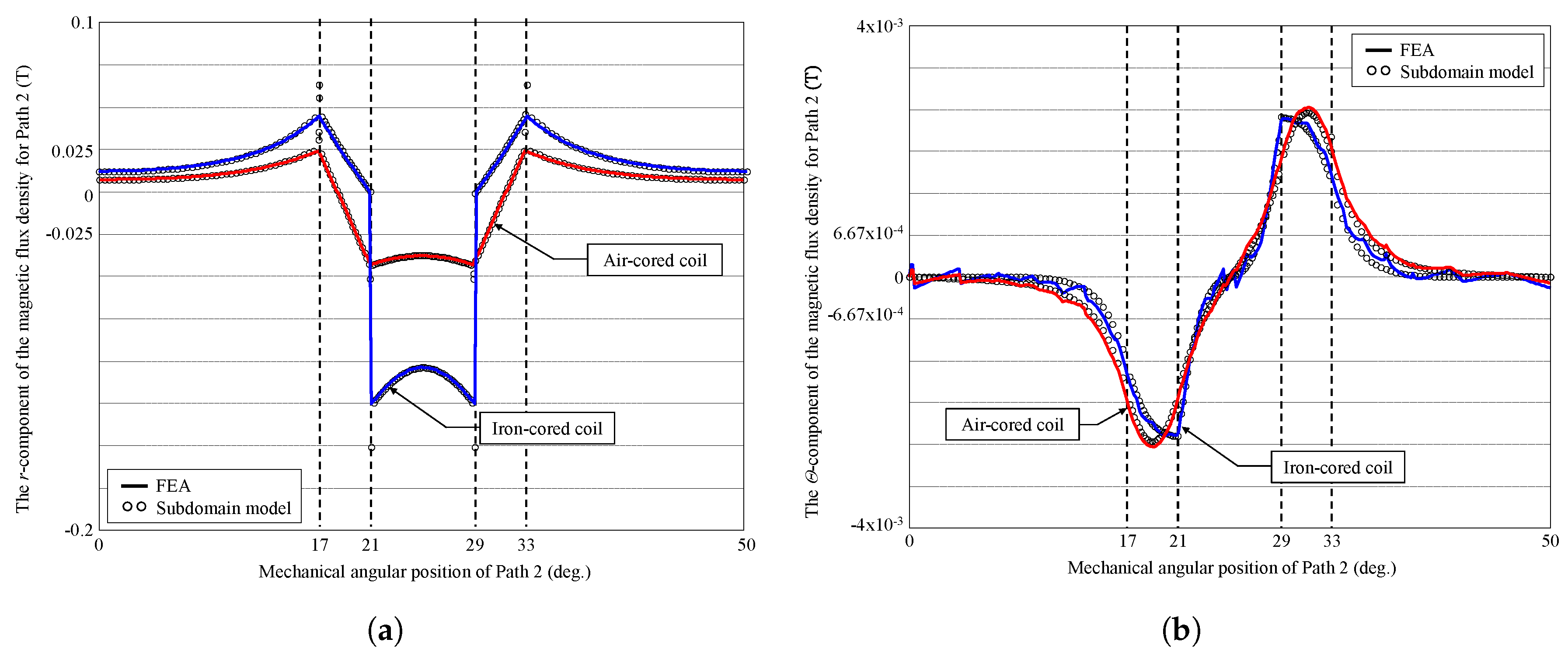
Figure 9.
Waveforms of for Path 3: (a) r- and (b) -component.

Figure 10.
Waveforms of for Path 4: (a) r- and (b) -component.

Figure 11.
Waveforms of for Path 5: (a) r- and (b) -component.


Table 1.
Physical and geometrical parameters of the air- or iron-cored coil.
| Parameters, Symbols (Units) | Values |
|---|---|
| Number of turns of the coil, (–) | 60 |
| Supply current, I (A) | 20 |
| Conductor surface, (mm) | 120 |
| Current density of the coil, (A/mm) | ±10 |
| Effective axial length, (mm) | 60 |
| Geometrical parameters in the -axis, (deg.) | |
| Geometrical parameters in the r-axis, (mm) | |
| Relative magnetic permeability of the iron, (–) | 1,500 |
| Number of harmonics for Region 1, (–) | 260 |
| Number of harmonics for Region 2, (–) | 260 |
| Number of harmonics for Region 3, (–) | |
| Number of harmonics for Region 4, (–) | |
| Number of harmonics for Region 5, (–) | |
| Number of harmonics for Region 6, (–) | |
| Number of harmonics for Region 7, (–) |
© 2017 by the authors. Licensee MDPI, Basel, Switzerland. This article is an open access article distributed under the terms and conditions of the Creative Commons Attribution (CC BY) license (http://creativecommons.org/licenses/by/4.0/).
Share and Cite
MDPI and ACS Style
Dubas, F.; Boughrara, K. New Scientific Contribution on the 2-D Subdomain Technique in Polar Coordinates: Taking into Account of Iron Parts. Math. Comput. Appl. 2017, 22, 42. https://doi.org/10.3390/mca22040042
AMA Style
Dubas F, Boughrara K. New Scientific Contribution on the 2-D Subdomain Technique in Polar Coordinates: Taking into Account of Iron Parts. Mathematical and Computational Applications. 2017; 22(4):42. https://doi.org/10.3390/mca22040042
Chicago/Turabian StyleDubas, Frédéric, and Kamel Boughrara. 2017. "New Scientific Contribution on the 2-D Subdomain Technique in Polar Coordinates: Taking into Account of Iron Parts" Mathematical and Computational Applications 22, no. 4: 42. https://doi.org/10.3390/mca22040042