Atmospheric Turbulence with Kolmogorov Spectra: Software Simulation, Real-Time Reconstruction and Compensation by Means of Adaptive Optical System with Bimorph and Stacked-Actuator Deformable Mirrors

Abstract

Atmospheric turbulence causes refractive index fluctuations, which in turn introduce extra distortions to the wavefront of the propagated radiation. It ultimately degrades telescope resolution (in imaging applications) and reduces radiation power density (in focusing applications). One of the possible ways of researching the impact of turbulence is to numerically simulate the spectrum of refractive index fluctuations, to reproduce it using a wavefront corrector and to measure the resultant wavefront using, for example, a Shack–Hartmann sensor. In this paper, we developed turbulence simulator software that generates phase screens with Kolmogorov spectra. We reconstructed the generated set of phase screens using a stacked-actuator deformable mirror and then compensated for the introduced wavefront distortions using a bimorph deformable mirror. The residual amplitude of the wavefront reconstructed by the 19-channel stacked-actuator mirror was 0.26 λ, while the residual amplitude of the wavefront compensated for by the 32-channel bimorph mirror was 0.08 λ.

1. Introduction

It is well known that turbulence leads to refractive index fluctuations, which in turn lead to extra distortions of the wavefront of the radiation that propagates through the atmosphere. Atmospheric turbulence limits the resolution of telescopes and decreases the coherence of laser radiation [1,2,3,4,5,6,7,8,9]. As a result, the quality of the image of the objects observed by the telescopes degrades. Other tasks that turbulence affects are the wireless transmission of energy and information with the help of optical radiation [10,11,12,13]. This is important, in particular, for recharging batteries at remote sites; the organization of optical communication channels in free space [14]; wireless optical communication, wireless power delivery to flying objects [15,16] and low-earth-orbit satellites [11]; providing a backup power supply and wireless power supply for household and industrial devices; destroying unmanned aerial vehicles or space debris [17,18,19]; providing communication with aircraft (in order to monitor their condition and obtain information); creating a beam of the desired shape [20]; focusing a beam inside a limited-aperture pinhole for laser communication tasks [21]; increasing the radiation power density on a target (laser cutting); and improving the accuracy of beam positioning (optical recording of information on media).

As is known, the low efficiency of systems for the wireless transmission of energy and information using optical-range radiation is due to light beam diffraction, radiation scattering by atmospheric aerosol [22], and the influence of atmospheric turbulence [23,24,25,26,27,28,29,30,31,32,33,34,35]. When a laser beam passes through the turbulent atmosphere of the Earth, the wavefront becomes distorted, which limits the operational range of such systems [36]. This problem has been studied for more than a dozen years, yet has not lost its relevance. The technology for increasing the efficiency of laser radiation transmission to the receiver includes two main components: high-quality efficient single-mode laser radiation sources and adaptive optical systems for correcting for wavefront aberrations [37,38]. In this research, we will concentrate on the second component.

The problems of increasing the range of the propagation of laser radiation through the atmosphere using adaptive optics methods are being solved by research teams from Russia, Germany, Italy, the USA, and the Netherlands [39,40,41]. In terms of adaptive optics for astronomical applications, we begin with the Air Force Maui Optical Station (AMOS) [42] in Hawaii, USA, where the ADONIS (Daylight Optical Near-Infrared System) system was built in 1993–1995. This system was placed in a 1.2 m telescope and was used to increase the quality of the obtained images of the astronomical objects. There were no adaptive optics inside this system since it used postprocessing. After that, the ADONIS system was moved to the 3.6 m EOAR telescope and was equipped with an adaptive optical system.

In [43,44], the authors describe a vision system that uses a conventional adaptive optical system and works on the 2.5 km horizontal atmospheric path. Another vision system with adaptive optics included, produced in the Fraunhofer Institute [45,46], was developed to run in urban conditions. The adaptive system contained a conventional deformable mirror and works with a frequency of 800 Hz. In [47], the authors describe the use of an adaptive optical system within an 0.35 m telescope on the 20 km slant atmospheric path. In [48], the authors describe an adaptive system with a deformable mirror and tip-tilt corrector for a 0.12 m telescope on the 3 km horizontal atmospheric path.

Most of the papers described above are devoted to the compensation of turbulence phase fluctuations. In this paper, we will first numerically simulate the effect of the specific turbulent atmosphere conditions on the wavefront of laser radiation. The second step is to reconstruct the simulated distortions using the stacked-actuator deformable mirror in laboratory conditions, followed by compensating for introduced distortions using the bimorph deformable mirror. Such a numerical–experimental simulation could allow us to estimate the influence of different turbulence conditions on the radiation wavefront and estimate the efficiency of the wavefront corrector.

2. Materials and Methods

2.1. Experimental Setup

The principal optical scheme of the adaptive system for atmospheric turbulence simulation and compensation is presented in Figure 1.

A point source (a fiber-coupled diode laser with a wavelength of 1.064 μm) is collimated with an achromatic lens to increase the beam diameter. The collimated laser beam is then incident on the 35 mm stacked-actuator deformable mirror with 19 control actuators, which introduces the phase delay in order to simulate the atmospheric turbulence. The distorted beam passes through the telescope (2 lenses), which optically conjugates the plane of the reflective surface of the stacked-actuator mirror with the plane of the bimorph mirror, and falls on the 30 mm bimorph deformable mirror with 32 control electrodes, which compensates for the introduced distortions. The corrected beam passes through the matching telescope and hits the Shack–Hartmann wavefront sensor.

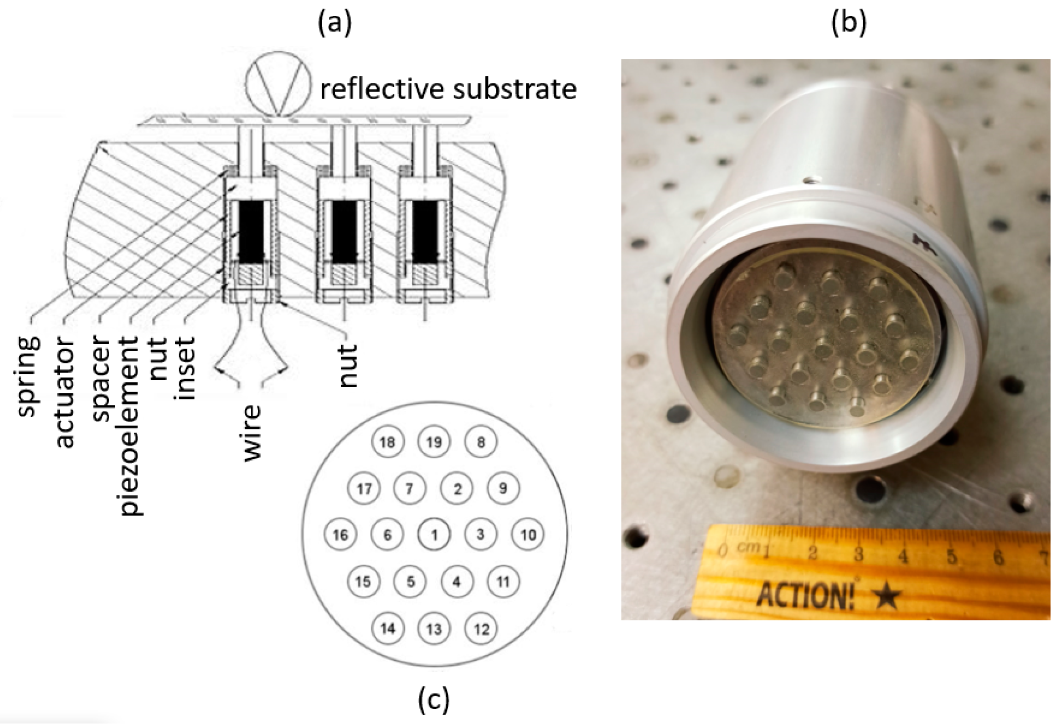
2.2. Stacked-Actuator Deformable Mirror

The scheme of the actuator’s layout and the principal scheme of the stacked-actuator mirror are presented in Figure 2, while the main mirror parameters are given in

Table 1. Main parameters of the stacked-actuator deformable mirror.

Parameter	Value
Substrate aperture	40 mm
Clear aperture	35 mm
Substrate material	glass
No. of control actuators	19
Type of actuators	PZT
Actuators geometry	Hexagonal
Maximum input voltage	−30…+130 V

.

There are a number of advantages of the stacked-actuator mirror. The first is the ability to replace individual actuators. If one actuator fails, there is no need to remove the substrate with the reflecting coating from all the other actuators—it is only necessary to unscrew the body of the broken actuator, keeping the tip of the actuator glued to the substrate, and then replace it with the working one. Secondly, the stacked-actuator mirror has the ability to polish the substrate in order to flatten the initial surface of the mirror in the assembled state, i.e., when all the actuator tips are glued to the substrate. The advantage of this mirror is that it requires a rather small initial adjustment of the surface in the assembled state, which preserves the dynamic range of the actuators for correcting the laser beam aberrations rather than the self-aberrations.

The bimorph mirror could also be used as a turbulence simulator. However, there are a few reasons why the stacked-actuator is a better choice. The first reason why the stacked-actuator mirror was used instead of a bimorph one for the reconstruction of the phase screens is that the bimorph mirror has a limited capacity to reproduce tilt aberrations, which have a big impact on the turbulent wavefront distortions. The stacked-actuator mirror, on the contrary, can reproduce the tilt aberrations without any significant sacrifice of dynamic range. The second reason is that it was interesting for us to test the efficiency of the newly developed stacked-actuator mirror.

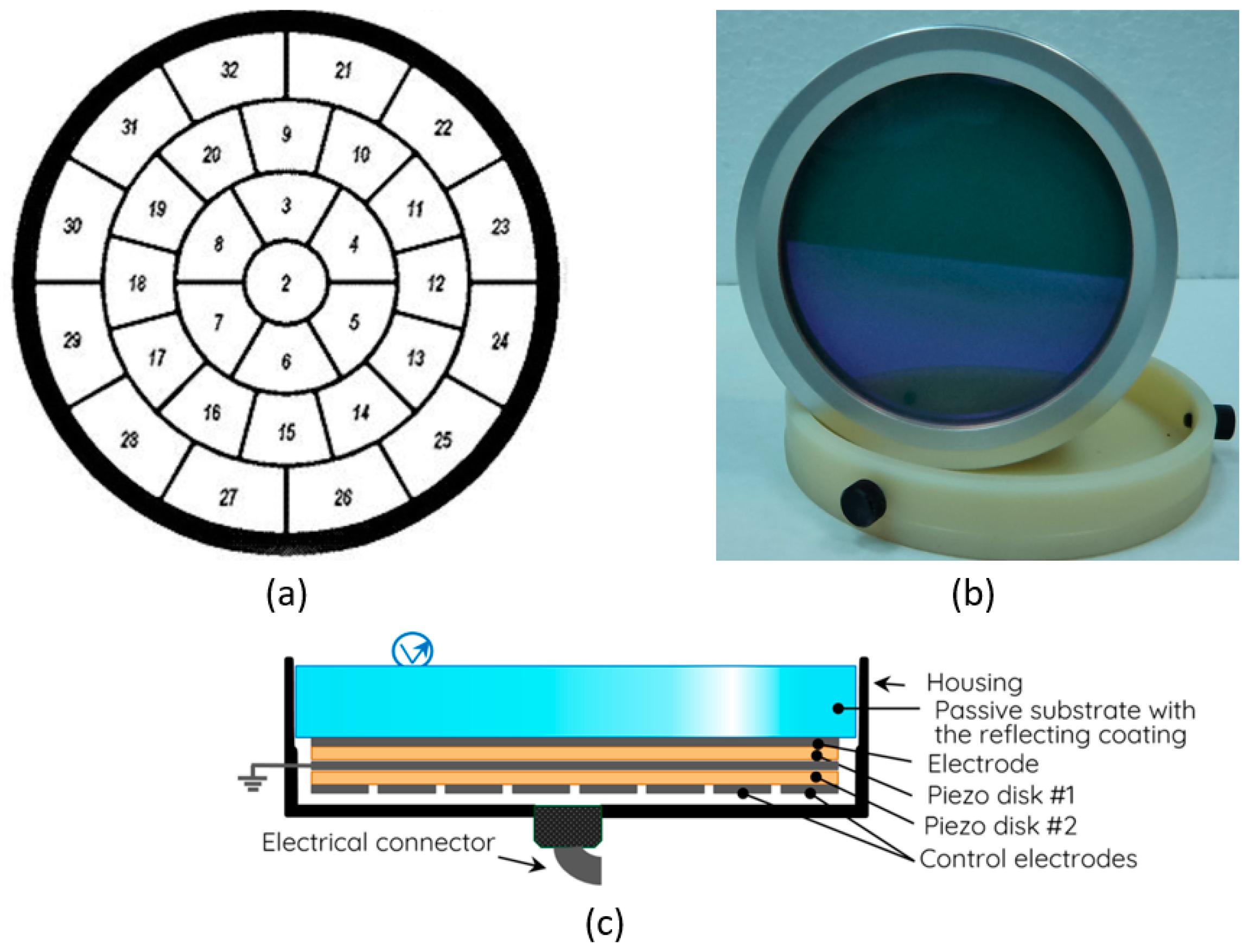
2.3. Bimorph Deformable Mirror

A bimorph mirror consists of a passive glass substrate with a reflective coating and two piezoceramic disks glued to it [49,50]. A common electrode is applied to the internal piezoceramic disk, which is designed to change the curvature of the reflecting surface of the mirror. A grid of control electrodes is applied to the external piezoceramic disk. The number of control electrodes depends on the type of aberrations to be compensated [51,52]. The scheme of the electrode dislocation and the principal scheme of the bimorph mirror are presented in Figure 3, while the main mirror parameters are given in

Table 2. Parameters of the bimorph deformable mirror.

Parameter	Value
Substrate aperture	35 mm
Clear aperture	30 mm
Substrate material	glass
No. of PZT	2
No. of control electrodes	32
Type of actuators	PZT discs
Actuators geometry	sectorial
Maximum input voltage	−200…+300 V

.

2.4. Shack–Hartmann Wavefront Sensor

In order to estimate the wavefront aberrations introduced by either the stacked-actuator or the bimorph deformable mirror, the Shack–Hartmann wavefront sensor [53,54,55,56,57,58] was used. The Shack–Hartmann wavefront sensor is a well-known device. It is quite simple to operate and can be easily calibrated for proper use [59]. Shack–Hartmann sensor is widely used in a large and diverse sets of applications, primarily to measure distortions of the wavefront of the radiation passing through different media, i.e., turbulent or scattering atmosphere [60], biological tissues [61], etc.

The principle of a conventional Shack–Hartmann sensor can be described as follows. The wavefront of the incident light is divided into a number of sub-apertures with the micro lens array. The micro lens array is a thin, flat base on which a grid of micro lenses is etched. Each micro lens has a diameter of 100 to 300 µm and a focal length f of 3 mm to 8 mm. Light passes through these micro lenses and creates a set of focal spots at the measurement (sensor) plane.

Since the diameter of each micro lens is small, the wavefront W is assumed to be flat and to have only tip-tilt aberration within a single micro lens. In the case of no aberrations (i.e., a wavefront is flat and parallel to the plane of the micro lens), the radiation is focused at the center of the corresponding sub-aperture of the sensor. If the wavefront in a micro lens has a non-zero tip-tilt, then the focal spot is displaced (S_x and S_y) from the center of the sub-aperture in proportion to the tip-tilt value. In other words, if we measure these displacements, S_x and S_y, of the focal spot per the X and Y axis, we will correspondingly obtain the values of the partial derivatives ∂W/∂x and ∂W/∂y of the wavefront W within each sub-aperture. On the other hand, to describe and visualize the wavefront surface analytically, one can use the polynomial approximation, for example, B-Splines [62] or Zernike polynomials [63,64,65,66], which are commonly used in optics. Thus, the partial wavefront derivatives ∂W/∂x and ∂W/∂y can be defined analytically using Zernike polynomials. They can also be calculated from the measured displacements S_x and S_y of the focal spots on the Shack–Hartmann sensor. Finally, we determined the overdetermined system of linear equations with the unknown coefficient’s $a_i$. By solving the least squares problem [67], we obtain the coefficient’s $a_i$. From here on, the wavefront can be analytically described and analyzed.

In addition to the wavefront measurements, the Shack–Hartmann sensor was used in order to measure the response functions of the actuators of our deformable mirrors (bimorph and stacked actuators one). Each control electrode or actuator is described by its own response function. The response function is a change in the profile of the mirror surface in response to the application of an electrical voltage to the electrode/actuator, while the remaining electrodes/actuators have a voltage under zero. The response function is presented as a set of focal spot displacements registered on the Shack–Hartmann wavefront sensor. Such a notation allows us to approximate the arbitrary wavefront measured by the Shack–Hartmann sensor (also presented as a set of focal spot displacements) using the response functions of the mirror.

2.5. Algorithm of Phase Screens Simulation

The main idea of this research is to simulate the set of phase screens with Kolmogorov spectra, to approximate and reproduce these phase screens using the 19-element stacked-actuator deformable mirror, and then to compensate for the introduced wavefront distortions using the 32-electrode bimorph deformable mirror.

In essence, the disturbance of an optical wave by a thin phase screen is the simplest model of the propagation in a turbulent atmosphere [68]. The fluctuations of the wave passing through a phase screen are similar to the fluctuations of the light field in a continuous randomly inhomogeneous medium. The thin phase screen most closely reproduces the influence of large-scale atmospheric inhomogeneities on the characteristics of the light field. In addition, the advantage of the phase screen method is that it allows the adaptive optical system to be analyzed to compensate for low-order phase aberrations in the atmosphere [69]. In other words, the phase screen approach is simple and presents a good approximation, and in most cases, it can reproduce the effect of turbulence on the wavefront with acceptable accuracy.

As a first step, we simulated the set of phase screens. To do this, we applied the Fast Fourier transform to the Kolmogorov spectrum of the phase fluctuations [70]:

$$p\left(u,v,t+∆t\right)={\iint }_{-\infty }^{\infty }\sqrt{K(x,y)}·f(x,y,t+∆t)·e^{i·\sqrt{x^2+y^2}·V·∆t}dxdy,$$

(1)

where $p\left(u,v,t+∆t\right)$ is the phase screen at moment $t+∆t$, $(x,y)$ is a spectrum point, $(u,v)$ is a phase screen point, $V$ is the wind velocity, m/s, $t$ is the moment of the previous phase screen generation, $t+∆t$ is the time moment of the new phase screen generation, $∆t$ is the time interval between two phase screens and $K(x,y)$ is the spectrum of the phase fluctuations.

The spectrum of the phase fluctuations $K(x,y)$ is calculated as follows:

$$K\left(x,y\right)=0.023·{\left(\frac{2D}{r_0}\right)}^{\frac{5}{3}}·{(x^2+y^2)}^{\frac{11}{3}},$$

(2)

where $D$ is the receiving aperture of the telescope, $r_0$ is the Fried radius and $f(x,y,t+∆t)$ is the function, defined as follows:

$$f\left(x,y,t+∆t\right)=p·f\left(x,y,t\right)+\sqrt{1-p^2}·e^{i·\phi (x,y,t)},$$

(3)

where $p=e^{\raisebox{1ex}{$-∆t$}\!\left/ \!\raisebox{-1ex}{$\tau $}\right.}$, $\tau$ is the coherence (or freezing) time of the atmosphere, $\phi (x,y,t)$ is the random delta-correlated value in the range of [0; 2π].

When $t=0$, the function $f$ is expressed as:

$$f\left(x,y,t=0\right)=e^{i·\phi (x,y,t=0)}.$$

(4)

The calculated phase values should be normalized in accordance with the relation $\frac{D}{r_0}$ [47]. We used the phase structure function to do this:

$$DN=6.88·{(\frac{\sqrt{x^2+y^2}}{r_0})}^{\frac{5}{3}}.$$

(5)

Each calculated phase screen was then approximated using the response functions of the stacked-actuator mirror and reproduced by this mirror. The response function of the individual actuator of the stacked-actuator deformable mirror represented the deformation of the surface of the mirror influenced by the voltage applied to this particular actuator, while other actuators still had a voltage under 0. In our case, the response function of each actuator of the mirror was measured by the Shack–Hartmann sensor and expressed as the vector of the displacements of the focal spots on the sensor.

Once the response functions of the mirror were measured, we could run the procedure of the reproduction of the particular phase screen by the mirror, described as follows:

• As we had the Zernike approximation of the simulated phase screen, we could calculate the values of the wavefront derivatives in each sub-aperture of the wavefront sensor.
• Knowing the values of the wavefront derivatives, we could calculate the displacements of the focal spots corresponding to these derivatives.
• Thus, knowing the focal spot shifts associated with the mirror response functions and the focal spot displacements corresponding to the wavefront to be reproduced, we could solve the overdetermined system of linear equations using the least squares method and calculate the vector of voltages that had to be applied to the mirror actuators.

After applying the calculated set of voltages to the mirror actuators, we reconstructed the desired phase screen. The accuracy of the reconstruction is provided in the Results section.

2.6. Algorithm of Phase Screen Compensation

Once the phase screen was reconstructed by the stacked-actuator deformable mirror, the correction procedure ran. It includes the following steps:

• The wavefront of the laser beam reflected from the stacked-actuator and bimorph mirrors was analyzed on the Shack–Hartmann wavefront sensor.
• Having, on the one hand, the matrix of displacements of the focal spots on the Shack–Hartmann sensor $\left\{\begin{array}{c}{S}_x^k\\ S_y^k\end{array}\right\}$, corresponding to the wavefront of the reconstructed phase screen, and, on the other hand, the matrix of values of the bimorph mirror response functions RF, also consisting of the focal spots shifts, we obtained an overdetermined system of linear equations for unknown coefficients, which were the values of the voltages at the mirror electrodes. To solve this system of equations, the least squares method was used.
• The calculated voltages were applied to the electrodes of the bimorph mirror.
• The residual wavefront was measured by means of the Shack–Hartmann sensor.

After the bimorph mirror compensated for the induced wavefront distortions, the phase screen simulation algorithm proceeded, and the described procedures were repeated.

3. Results and Discussion

The experiment was conducted as follows:

• Simulation of the set of phase screens using the Fast Fourier transform for the Kolmogorov spectrum of phase fluctuations [71,72].
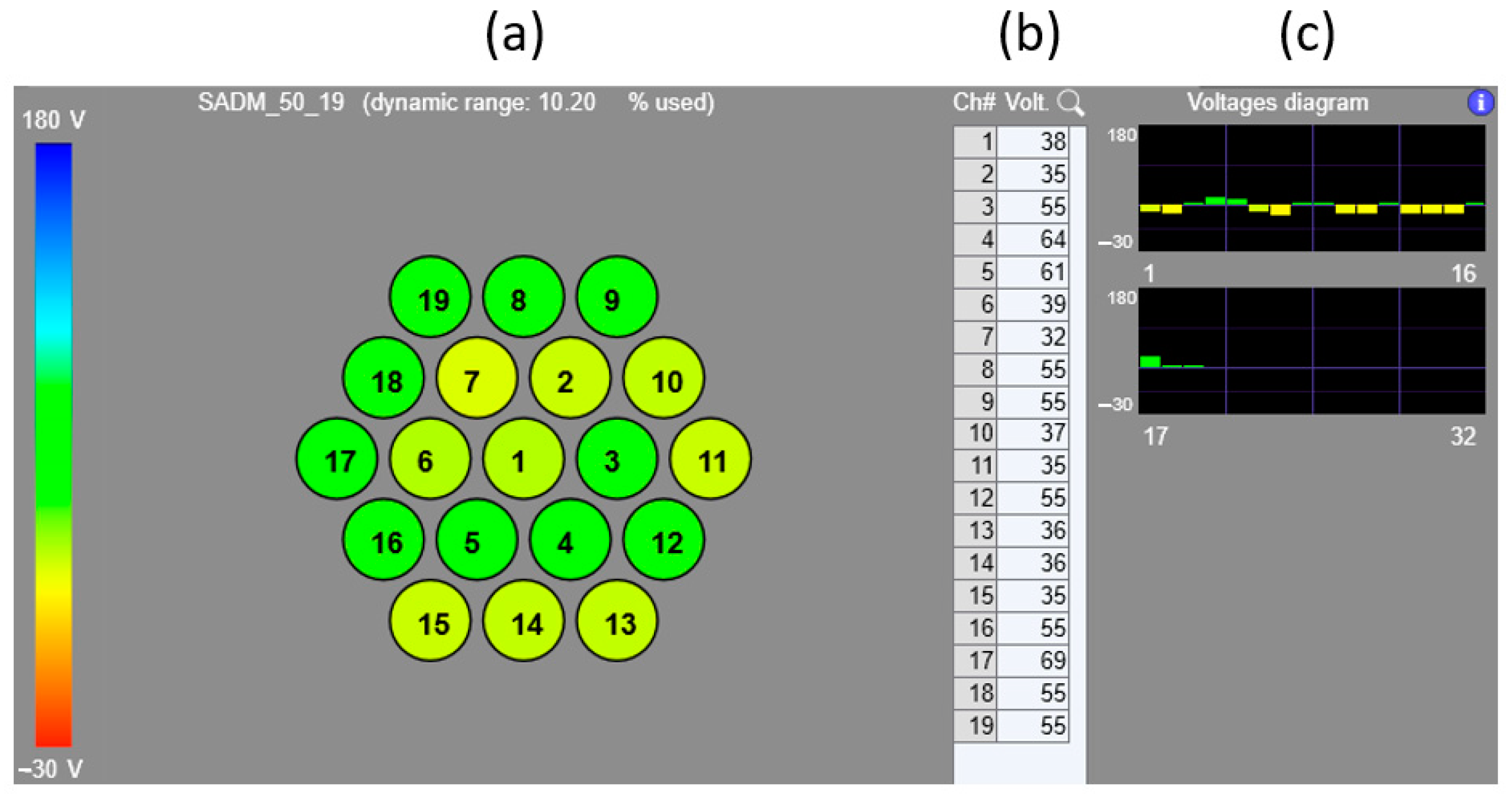
• Calculation of the control voltages to be applied to the actuators of the stacked-actuator deformable mirror [73].
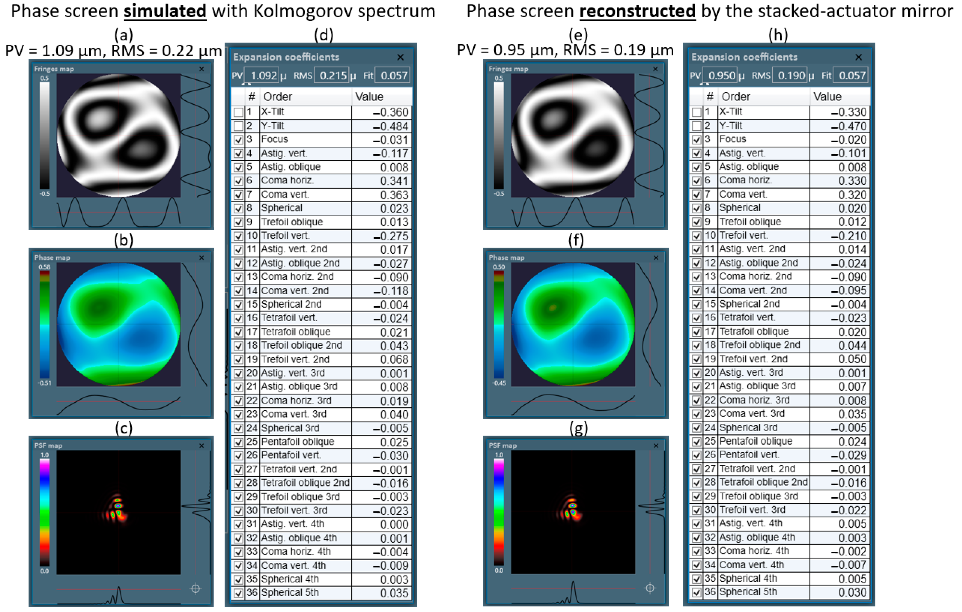
• Reconstruction of the simulated phase screens using the stacked-actuator mirror.
• Measurement of the introduced wavefront distortions using the Shack–Hartmann wavefront sensor.
• Calculation of the control voltages to be applied to the electrodes of the bimorph deformable mirror in order to compensate for the wavefront distortions.
• Compensation of the reconstructed phase screens by the bimorph mirror.

It is well known that the main parameter characterizing the strength of atmospheric turbulence is the refractive index structure parameter $C_n^2$. It can vary from ${10}^{-17}{\mathrm{m}}^{-\frac{2}{3}}$ for weak turbulence to ${10}^{-12}{\mathrm{m}}^{-\frac{2}{3}}$ for very strong atmospheric turbulence. For example, in Hefei city, China, $C_n^2$ varies from $6.69\times {10}^{-16}{\mathrm{m}}^{-\frac{2}{3}}$ to $9.87\times {10}^{-14}{\mathrm{m}}^{-\frac{2}{3}}$ for measurements performed in the summer month at 1 km horizontal atmospheric path [74]. For maritime atmospheric turbulence $C_n^2$ is equal to ${10}^{-15}{\mathrm{m}}^{-\frac{2}{3}}$ for the 10 km path, coherence radius $r_0=3.8 \mathrm{c}\mathrm{m}$ for laser wavelength $\lambda =0.85 \mathsf{\mu }\mathrm{m}$ [75]. For ground-to-space communication between the International Space Station and the Optical Communications Telescope Laboratory (OCTL) in Wrightwood, California, a coherence radius of $r_0=4.5 \mathrm{c}\mathrm{m}$ has been experimentally measured for the 1200 km path and 75° zenith angle, with the input telescope aperture varied from $10 \mathrm{c}\mathrm{m}$ to $100 \mathrm{c}\mathrm{m}$ [76]. For terrestrial atmospheric turbulence $C_n^2$ is equal to ${10}^{-12}{\mathrm{m}}^{-\frac{2}{3}}$ for the 1 km path, where the wind velocity was 10 m/s and the telescope aperture was 20 cm [77]. For desert atmospheric turbulence, $C_n^2$ is equal to ${10}^{-13.2}{\mathrm{m}}^{-\frac{2}{3}}$ (for an average wind velocity of 6 m/s) for 1.2 km path at Edward Air Force Base, Mojave Desert, CA, USA [78]. For the atmospheric turbulence measured by our team in collaboration with our Austrian colleagues at the 1.2 km intra-city link in Vienna, Austria, the coherence radius was equal to $r_0=1.6 \mathrm{c}\mathrm{m}$ for the laser wavelength $\lambda =0.532 \mathsf{\mu }\mathrm{m}$ and $r_0=2.65 \mathrm{c}\mathrm{m}$ for $\lambda =0.81 \mathsf{\mu }\mathrm{m}$; the wind velocity varied from 5 to 10 m/s for the receiving aperture D = 140 mm.

However, $C_n^2$ can be calculated from the known receiving aperture diameter D and Fried radius $r_0$. In this research we set $\frac{D}{r_0}=10$, the wavelength λ = 1 μm, and the wind velocity v = 6 m/s. $C_n^2$ varies roughly from $9\times {10}^{-15}{\mathrm{m}}^{-\frac{2}{3}}$ to $8\times {10}^{-14}{\mathrm{m}}^{-\frac{2}{3}}$ for the path length from 500 m to 3 km.

Figure 4 presents the results of the Zernike approximation of the phase screen simulated with the Kolmogorov spectrum and the results of the reconstruction of this phase screen with the stacked-actuator deformable mirror.

The input parameters for the phase screens simulation algorithm were as follows:

It can be seen from Figure 4 that the stacked-actuator deformable mirror reconstructs the simulated phase surface with an error of about 13%. The amplitude of the wavefront distortions of the approximated phase screen was equal to 1.09 μm (root mean square error RMS = 0.22 μm). The amplitude of the reconstructed surface was equal to 0.95 μm (RMS = 0.19 μm). The voltages on the actuators of the stacked-actuator mirror required to reconstruct such a wavefront are presented in Figure 5.

It should be noted that the voltage range for the stacked-actuator mirror is −30 V–+180 V. This means that in order to use the whole dynamic range, we have to set the offset voltages for each actuator. In our case, the offset voltage was 50 V. It can be seen from Figure 5 that the voltage values required to reconstruct the desired wavefront shape were not very high—the voltage variation was about ±20 V. It took only 10% of the dynamic range of the mirror, where 100% of the dynamic range means that either −30 V or +180 V is applied for each actuator. This is due to high-sensitivity of the piezoceramic actuators used in the mirror. The 13% error of the phase screen reconstruction is mainly because of the limited number of the actuators used in the mirror.

In order to estimate the accuracy of the reconstruction, we subtracted the raw phase data of the reconstructed screen from the raw phase data of the simulated phase screen. The resultant phase difference surface is presented in Figure 6.

Such a difference (PV = 0.26 μm) between the simulated and reconstructed phase surfaces may be due, first of all, to a hysteresis effect of piezoceramics used in the actuators of the mirror [79]. In essence, the response of the actuators of the stacked-actuator mirror is on average 15% smaller/bigger than the expected response for each act of voltage application. Thus, it takes 2–3 iterations to compensate for the hysteresis and reduce the phase delay between the expected and real phase screen.

The second step was to compensate for the introduced wavefront distortions with the bimorph deformable mirror. Figure 7 shows the result of the compensation of the phase screen with the bimorph mirror.

The 35 mm diameter bimorph deformable mirror with 32 control electrodes compensates for the introduced distortions with high efficiency. The residual wavefront amplitude was equal to 0.08 μm, while the RMS was only 0.01 μm (λ/100).

The voltages on the electrodes of the bimorph mirror were required to compensate for the wavefront distortions introduced by the stacked-actuator mirror are presented in Figure 8.

It can be seen from Figure 8 that the voltage values required to compensate for the induced wavefront distortions were higher than for the stacked-actuator mirror—the voltage change was about ±100 V. It took about 9% of the dynamic range of the mirror, where 100% of the dynamic range means that either −300 V or +300 V is applied to each electrode.

Since the efficiency of the currently used 19-channel stacked-actuator mirror as a phase screen reconstruction device was not very high (the reconstruction error was about 13%), the first step for future research will be to increase the number of actuators of the stacked-actuator mirror. In addition, the amplitude of the phase fluctuations of the simulated phase screens can be increased in order to test both the efficiency and stability of the compensation loop.

4. Conclusions

In this research, turbulence simulator software was developed and tested to generate phase screens with Kolmogorov spectra. The set of phase screens was generated for the ratio of receiving telescope aperture to Fried radius equal to $10$, a wavelength equal to 1 μm, and a wind velocity equal to 6 m/s. The refractive index structure parameter $C_n^2$ varied roughly from $9\times {10}^{-15}{\mathrm{m}}^{-\frac{2}{3}}$ to $8\times {10}^{-14} {\mathrm{m}}^{-\frac{2}{3}}$ for the path length from 500 m up to 3000 m. The generated set of phase screens was reconstructed using the 19-channel stacked-actuator deformable mirror and then compensated for using the 32-channel bimorph deformable mirror. It was shown that the residual amplitude of the wavefront reconstructed by the 19-channel stacked-actuator mirror was 0.26 λ, while the residual amplitude of the wavefront compensated by the 32-channel bimorph mirror was 0.08 λ.

References

1. Tatarsky, V.I. Waves Propagation in Turbulent Atmosphere; Nauka: Moscow, Russia, 1967. [Google Scholar]
2. Andrews, L.C.; Phillips, R.L. Laser Beam Propagation Through Random Media, 2nd ed.; SPIE Press: Bellingham, WA, USA, 2005. [Google Scholar]
3. Huang, Q.; Liu, D.; Chen, Y.; Wang, Y.; Tan, J.; Chen, W.; Liu, J.; Zhu, N. Secure free-space optical communication system based on data fragmentation multipath transmission technology. Opt. Express 2018, 26, 13536–13542. [Google Scholar] [CrossRef] [PubMed]
4. Nafria, V.; Han, X.; Djordjevic, I. Improving free-space optical communication with adaptive optics for higher order modulation. In Proceedings of the Optics and Photonics for Information Processing XIV, Online, CA, USA, 24 August–4 September 2020. [Google Scholar]
5. Vorontsov, M.; Weyrauch, T.; Carhart, G.; Beresnev, L. Adaptive Optics for Free Space Laser Communications. In Lasers, Sources and Related Photonic Devices, OSA Technical Digest Series (CD); Optica Publishing Group: Washington, DC, USA, 2010; p. LSMA1. [Google Scholar]
6. Weyrauch, T.; Vorontsov, M. Free-space laser communications with adaptive optics: Atmospheric compensation experiments. J. Optic. Comm. Rep. 2004, 1, 355–379. [Google Scholar] [CrossRef]
7. Lema, G. Free space optics communication system design using iterative optimization. J. Opt. Commun. 2020, 000010151520200007. [Google Scholar] [CrossRef]
8. Zhang, Y.; Wang, Y.; Deng, Y.; Du, A.; Liu, J. Design of a Free Space Optical Communication System for an Unmanned Aerial Vehicle Command and Control Link. Photonics 2021, 8, 163. [Google Scholar] [CrossRef]
9. Majumdar, A. Fundamentals of Free-Space Optical (FSO) Communication System. In Advanced Free Space Optics (FSO); Series in Optical Sciences; Springer: New York, NY, USA, 2015; Volume 186. [Google Scholar]
10. Lu, M.; Bagheri, M.; James, A.P.; Phung, T. Wireless Charging Techniques for UAVs: A Review, Reconceptualization, and Extension. IEEE Access 2018, 6, 29865–29884. [Google Scholar] [CrossRef]
11. Geoffrey, A.; Landis, H. Laser beamed power—Satellite demonstration applications. In Proceedings of the 43rd International Astronautical Congress, Washington, DC, USA, 28 August–5 September 1992. [Google Scholar]
12. Vorontsov, M.; Weyrauch, T.; Carhart, G. Lasers, Sources and Related Photonic Devices; OSA Technical Digest Series (CD); Optica Publishing Group: San Diego, USA, 2010; p. LSMA1. [Google Scholar]
13. Galaktionov, I.; Kudryashov, A.; Sheldakova, J.; Nikitin, A. Laser beam focusing through the scattering medium by means of adaptive optics. In Proceedings of the Adaptive Optics and Wavefront Control for Biological Systems III, San Francisco, CA, USA, 28 January–2 February 2017. [Google Scholar]
14. Wang, R.; Wang, Y.; Jin, C.; Yin, X.; Wang, S.; Yang, C.; Cao, Z.; Mu, Q.; Gao, S.; Xuan, L. Demonstration of horizontal free-space laser communication with the effect of the bandwidth of adaptive optics system. Opt. Commun. 2018, 431, 167–173. [Google Scholar] [CrossRef]
15. Chittoor, P.K.; Chokkalingam, B.; Mihet-Popa, L. A Review on UAV Wireless Charging: Fundamentals, Applications, Charging Techniques and Standards. IEEE Access 2021, 9, 69235–69266. [Google Scholar] [CrossRef]
16. Wang, C.; Ma, Z. Design of wireless power transfer device for UAV. In Proceedings of the 2016 IEEE International Conference on Mechatronics and Automation, Harbin, China, 7–10 August 2016; pp. 2449–2454. [Google Scholar]
17. Bennet, F.; Conan, R.; D’Orgeville, C.; Dawson, M.; Paulin, N.; Price, I.; Rigaut, F.; Ritchie, I.; Smith, C.; Uhlendorf, K. Adaptive optics for laser space debris removal. In Proceedings of the Adaptive Optics Systems III, Amsterdam, The Netherlands, 1–6 July 2012. [Google Scholar]
18. Phipps, C.R.; Baker, K.L.; Libby, S.B.; Liedahl, D.A.; Olivier, S.S.; Pleasance, L.D.; Rubenchik, A.; Trebes, J.E.; George, E.V.; Marcovici, B.; et al. Removing orbital debris with lasers. Adv. Space Res. 2012, 49, 1283–1300. [Google Scholar] [CrossRef]
19. Shen, S.; Jin, X.; Hao, C. Cleaning space debris with a space-based laser system. Chin. J. Aeronaut. 2014, 27, 805–811. [Google Scholar] [CrossRef]
20. Sheldakova, J.; Galaktionov, I.; Nikitin, A.; Rukosuev, A.; Kudryashov, A. LC phase modulator vs deformable mirror for laser beam shaping: What is better? In Proceedings of the Laser Beam Shaping XVIII, San Diego, CA, USA, 19–23 August 2018; Volume 10744, pp. 156–162. [Google Scholar]
21. Galaktionov, I.; Nikitin, A.; Sheldakova, J.; Toporovsky, V.; Kudryashov, A. Focusing of a Laser Beam Passed through a Moderately Scattering Medium Using Phase-Only Spatial Light Modulator. Photonics 2022, 9, 296. [Google Scholar] [CrossRef]
22. Galaktionov, I.; Kudryashov, A.; Sheldakova, J.; Nikitin, A. The use of modified hill-climbing algorithm for laser beam focusing through the turbid medium. In Proceedings of the Laser Resonators, Microresonators, and Beam Control XIX, San Francisco, CA, USA, 28 January–2 February 2017. [Google Scholar]
23. Barros, R.; Keary, S. Experimental setup for investigation of laser beam propagation along horizontal urban path. Proc. SPIE 2014, 9242, 396–404. [Google Scholar]
24. Mata-Calvo, R. Transmitter diversity verification on Artemis geostationary satellite. In Proceedings of the Free-Space Laser Communication and Atmospheric Propagation XXVI, San Francisco, CA, USA, 1–6 February 2014. [Google Scholar]
25. Mosavi, N.; Marks, B.; Boone, B.; Menyuk, C. Optical beam spreading in the presence of both atmospheric turbulence and quartic aberration. In Proceedings of the Free-Space Laser Communication and Atmospheric Propagation XXVI, San Francisco, CA, USA, 1–6 February 2014. [Google Scholar]
26. Murty, S.S.R. Laser beam propagation in atmospheric turbulence. Proc. Indian Acad. Sci. 1979, 2, 179–195. [Google Scholar] [CrossRef]
27. Kwiecień, J. The effects of atmospheric turbulence on laser beam propagation in a closed space—An analytic and experimental approach. Opt. Commun. 2019, 433, 200–208. [Google Scholar] [CrossRef]
28. Searles, S.; Hart, G.; Dowling, J.; Hanley, S. Laser beam propagation in turbulent conditions. Appl. Opt. 1991, 30, 401–406. [Google Scholar] [CrossRef]
29. Gareth, D.; Naven, C. Experimental analysis of a laser beam propagating in angular turbulence. Open Phys. 2022, 20, 402–415. [Google Scholar]
30. Summerer, L.; Purcell, O. Concepts for wireless energy transmission via laser. J. Br. Interplanet. Soc. 2005, 58, 1–10. [Google Scholar]
31. Fahey, T.; Islam, M.; Gardi, A.; Sabatini, R. Laser Beam Atmospheric Propagation Modelling for Aerospace LIDAR Applications. Atmosphere 2021, 12, 918. [Google Scholar] [CrossRef]
32. Zohuri, B. Atmospheric Propagation of High-Energy Laser Beams. In Directed Energy Weapons; Springer: Cham, Switzerland, 2016. [Google Scholar]
33. Shuto, Y. Effect of Water and Aerosols Absorption on Laser Beam Propagation in Moist Atmosphere at Eye-Safe Wavelength of 1.57 µm. J. Electr. Electron. Eng. 2023, 11, 15–22. [Google Scholar]
34. Rosen, L.; Ipser, J. High Energy Laser Beam Scattering by Atmospheric Aerosol Aureoles. In Proceedings of the Nonlinear Optical Beam Manipulation and High Energy Beam Propagation through the Atmosphere, Los Angeles, CA, USA, 5–20 January 1989. [Google Scholar]
35. Oosterwijk, A.; Heikamp, S.; Manders-Groot, A.; Lex, A.; Eijk, J. Comparison of modelled atmospheric aerosol content and its influence on high-energy laser propagation. In Proceedings of the Laser Communication and Propagation through the Atmosphere and Oceans VIII, San Diego, CA, USA, 11–15 August 2019. [Google Scholar]
36. Kudryashov, A.; Rukosuev, A.; Samarkin, V.; Galaktionov, I.; Kopylov, E. Fast adaptive optical system for 1.5 km horizontal beam propagation. In Proceedings of the Unconventional and Indirect Imaging, Image Reconstruction, and Wavefront Sensing 2018, San Diego, CA, USA, 19–23 August 2018. [Google Scholar]
37. Soloviev, A.; Kotov, A.; Perevalov, S.; Esyunin, M.; Starodubtsev, M.; Alexandrov, A.; Galaktionov, I.; Samarkin, V.; Kudryashov, A.; Ginzburg, V.; et al. Adaptive system for wavefront correction of the PEARL laser facility. Quantum Electron. 2022, 50, 1115–1122. [Google Scholar] [CrossRef]
38. Samarkin, V.; Alexandrov, A.; Galaktionov, I.; Kudryashov, A.; Nikitin, A.; Rukosuev, A.; Toporovsky, V.; Sheldakova, Y. Large-aperture adaptive optical system for correcting wavefront distortions of a petawatt Ti:sapphire laser beam. Quantum Electron. 2022, 52, 187–194. [Google Scholar] [CrossRef]
39. Buck, A.L. Effects of the Atmosphere on Laser Beam Propagation. Appl. Opt. 1967, 6, 703–708. [Google Scholar] [CrossRef] [PubMed]
40. Galaktionov, I.; Kudryashov, A.; Sheldakova, J.; Nikitin, A.; Samarkin, V. Laser beam focusing through the atmosphere aerosol. In Proceedings of the Unconventional and Indirect Imaging, Image Reconstruction, and Wavefront Sensing 2017, San Diego, CA, USA, 6–10 August 2017; Volume 10410, pp. 152–165. [Google Scholar]
41. Lylova, A.; Kudryashov, A.; Sheldakova, J.; Borsoni, G. The real-time atmospheric turbulence modeling and compensation with the use of adaptive optics. In Proceedings of the Optics in Atmospheric Propagation and Adaptive Systems XVIII, Toulouse, France, 21–24 September 2015. [Google Scholar]
42. Gonglewski, J.; Highland, R.; Dayton, D.; Sandven, S.; Rogers, S.; Browne, S. ADONIS: Daylight Imaging through Atmospheric Turbulence. In Proceedings of the Digital Image Recovery and Synthesis III, Denver, CO, USA, 4–9 August 1996. [Google Scholar]
43. Marchi, G.; Weiß, R. Evaluations and Progress in the Development of an Adaptive Optics System for Ground Object Observation. In Proceedings of the Optics in Atmospheric Propagation and Adaptive Systems X, Florence, Italy, 17–20 September 2007. [Google Scholar]
44. Marchi, G.; Scheifling, C. Adaptive optics concepts and systems for multipurpose applications at near horizontal line of sight: Developments and results. In Proceedings of the Optics in Atmospheric Propagation and Adaptive Systems XII, Berlin, Germany, 31 August–3 September 2009. [Google Scholar]
45. Segel, M.; Gladysz, S.; Stein, K. Optimal modal compensation in gradient-based wavefront sensorless adaptive optics. In Proceedings of the Laser Communication and Propagation through the Atmosphere and Oceans VIII, San Diego, CA, USA, 11–15 August 2019. [Google Scholar]
46. Segel, M.; Zepp, A.; Anzuola, E.; Gladysz, S.; Stein, K. Optimization of wavefront-sensorless adaptive optics for horizontal laser beam propagation in a realistic turbulence environment. In Proceedings of the Laser Communication and Propagation through the Atmosphere and Oceans VI, San Diego, CA, USA, 6–10 August 2017. [Google Scholar]
47. Gonglewski, J.; Dayton, D. Least squares blind deconvolution of air to ground imaging. In Proceedings of the Optics in Atmospheric Propagation and Adaptive Systems VIII, Bruges, Belgium, 19–22 September 2005. [Google Scholar]
48. Mackey, R.; Dainty, C. Adaptive optics correction over a 3km near horizontal path. In Proceedings of the Optics in Atmospheric Propagation and Adaptive Systems XI, Cardiff, UK, 15–18 September 2008. [Google Scholar]
49. Sheldakova, J.; Toporovsky, V.; Galaktionov, I.; Nikitin, A.; Rukosuev, A.; Samarkin, V.; Kudryashov, A. Flat-top beam formation with miniature bimorph deformable mirror. In Proceedings of the Laser Beam Shaping XX, Online, CA, USA, 24 August–4 September 2020. [Google Scholar]
50. Samarkin, V.; Alexandrov, A.; Galaktionov, I.; Kudryashov, A.; Nikitin, A.; Rukosuev, A.; Toporovsky, V.; Sheldakova, J. Wide-Aperture Bimorph Deformable Mirror for Beam Focusing in 4.2 PW Ti:Sa Laser. Appl. Sci. 2022, 12, 1144. [Google Scholar] [CrossRef]
51. Galaktionov, I.; Nikitin, A.; Samarkin, V.; Sheldakova, J.; Kudryashov, A. Laser beam focusing through the scattering medium-low order aberration correction approach. In Proceedings of the Unconventional and Indirect Imaging, Image Reconstruction, and Wavefront Sensing 2018, San Diego, CA, USA, 19–23 August 2018. [Google Scholar]
52. Galaktionov, I.; Kudryashov, A.; Sheldakova, J.; Nikitin, A. Laser beam focusing through the dense multiple scattering suspension using bimorph mirror. In Proceedings of the Adaptive Optics and Wavefront Control for Biological Systems V, San Francisco, CA, USA, 20 February 2019; Volume 10886, p. 1088619. [Google Scholar]
53. Platt, B.; Shack, R.J. History and principles of Shack-Hartmann wavefront sensing. Refr. Surg. 2001, 17, 15. [Google Scholar] [CrossRef]
54. Liang, J.; Grimm, B.; Goelz, S.; Bille, J.F. Objective measurement of the wave aberrations of the human eye with the use of a Hartmann-Shack wave-front sensor. J. Opt. Soc. Am. A 1994, 11, 1949. [Google Scholar] [CrossRef]
55. Lane, R.G. Wave-front reconstruction using a Shack–Hartmann sensor. Appl. Opt. 1992, 31, 6902. [Google Scholar] [CrossRef]
56. Primot, J. Theoretical description of Shack–Hartmann wave-front sensor. Opt. Commun. 2003, 222, 81–92. [Google Scholar] [CrossRef]
57. Konnik, M.; Doná, J. Waffle mode mitigation in adaptive optics systems: A constrained Receding Horizon Control approach. In Proceedings of the American Control Conference, Washington, DC, USA, 17–19 June 2013; pp. 3390–3396. [Google Scholar]
58. Mauch, S.; Reger, J. Real-Time Spot Detection and Ordering for a Shack–Hartmann Wavefront Sensor with a Low-Cost FPGA. Proc. IEEE Trans. Instrum. Meas. 2014, 63, 2379–2386. [Google Scholar] [CrossRef]
59. Nikitin, A.; Galaktionov, I.; Sheldakova, J.; Kudryashov, A.; Baryshnikov, N.; Denisov, D.; Karasik, V.; Sakharov, A. Absolute calibration of a Shack-Hartmann wavefront sensor for measurements of wavefronts. In Proceedings of the Photonic Instrumentation Engineering VI, San Francisco, CA, USA, 2–7 February 2019. [Google Scholar]
60. Galaktionov, I.; Sheldakova, J.; Nikitin, A.; Toporovsky, V.; Kudryashov, A. A Hybrid Model for Analysis of Laser Beam Distortions Using Monte Carlo and Shack–Hartmann Techniques: Numerical Study and Experimental Results. Algorithms 2023, 16, 337. [Google Scholar] [CrossRef]
61. Galaktionov, I.; Kudryashov, A.; Sheldakova, J.; Byalko, A.; Borsoni, G. Laser beam propagation and wavefront correction in turbid media. In Proceedings of the Unconventional Imaging and Wavefront Sensing 2015, San Diego, CA, USA, 9–13 August 2015. [Google Scholar]
62. Galaktionov, I.; Nikitin, A.; Sheldakova, J.; Kudryashov, A. B-spline approximation of a wavefront measured by Shack-Hartmann sensor. In Proceedings of the Laser Beam Shaping XXI, San Diego, CA, USA, 1–5 August 2021. [Google Scholar]
63. Malacara-Hernandez, D. Wavefront fitting with discrete orthogonal polynomials in a unit radius circle. Opt. Eng. 1990, 29, 672–675. [Google Scholar] [CrossRef]
64. Wyant, J.C.; Creath, K. Basic wavefront aberration theory for optical metrology. In Applied Optics and Optical Engineering; Academic Press: Cambridge, MA, USA, 1992; pp. 28–39. [Google Scholar]
65. Genberg, V.; Michels, G.; Doyle, K. Orthogonality of Zernike polynomials. Proc. SPIE 2002, 4771, 276–287. [Google Scholar]
66. Lakshminarayanan, V.; Fleck, A. Zernike polynomials: A guide. J. Mod. Opt. 2011, 58, 545–561. [Google Scholar] [CrossRef]
67. Linnik, J.V. Least Square Error Method and the Basics of Mathematical-Statistical Theory, 2nd ed.; Mir: Moscow, Russia, 1962. [Google Scholar]
68. Kandidov, V.; Shlenov, A. Atmospheric Turbulence Simulation. Grid Representation. Technical Summary; International Laser Center: Moscow, Russia, 1995. [Google Scholar]
69. Vorontsov, M.; Shmalhausen, V. Principles of Adaptive Optics; Nauka: Moscow, Russia, 1985. [Google Scholar]
70. Dudorov, V.; Kolosov, V.; Filimonov, G. Algorithm for formation of an infinite random turbulent screen. In Proceedings of the Twelfth Joint International Symposium on Atmospheric and Ocean Optics/Atmospheric Physics, Tomsk, Russia, 27–30 June 2005. [Google Scholar]
71. Lane, R.G.; Glindemann, A.; Dainty, J.C. Simulation of Kolmogorov phase screen. Waves Random Media 1992, 2, 209–224. [Google Scholar] [CrossRef]
72. Burger, L.; Litvin, I.; Forbes, A. Simulating atmospheric turbulence using a phase-only spatial light modulator. South Afr. J. Sci. 2008, 104, 129–137. [Google Scholar]
73. Laslandes, M.; Patterson, K.; Pellegrino, S. Optimized actuators for ultrathin deformable primary mirrors. Appl. Opt. 2015, 54, 1559. [Google Scholar] [CrossRef] [PubMed]
74. Liu, D.; Wang, Z.; Liu, J.; Tan, J.; Yu, L.; Mei, H.; Zhou, Y.; Zhu, N. Performance analysis of 1-km free-space optical communication system over real atmospheric turbulence channels. Opt. Eng. 2017, 56, 106111. [Google Scholar] [CrossRef]
75. Li, M.; Cvijetic, M. Coherent free space optics communications over the maritime atmosphere with use of adaptive optics for beam wavefront correction. Appl. Opt. 2015, 54, 1453–1462. [Google Scholar] [CrossRef]
76. Wright, M.W.; Morris, J.F.; Kovalik, J.M.; Andrews, K.S.; Abrahamson, M.J.; Biswas, A. Adaptive optics correction into single mode fiber for a low Earth orbiting space to ground optical communication link using the OPALS downlink. Opt. Express 2015, 23, 33705–33712. [Google Scholar] [CrossRef] [PubMed]
77. Thompson, C.A.; Kartz, M.W.; Flath, L.M.; Wilks, S.C.; Young, R.A.; Johnson, G.W.; Ruggiero, A.J. Free space optical communications utilizing MEMS adaptive optics correction. In Proceedings of the Free-Space Laser Communication and Laser Imaging II, Seattle, WA, USA, 7–11 July 2002. [Google Scholar]
78. Majumdar, A.K.; Eaton, F.D.; Jensen, M.L.; Kyrazis, D.T.; Schumm, B.; Dierking, M.P.; Shoemake, M.A.; Dexheimer, D.; Ricklin, J.C. Atmospheric Turbulence Measurements over Desert site using groundbased instruments, kite/tethered-blimp platform and aircraft relevant to optical communications and imaging systems: Preliminary Results. In Proceedings of the Free-Space Laser Communications VI, San Diego, CA, USA, 13–17 August 2006. [Google Scholar]
79. Cornelissen, S.; Hartzell, A.; Stewart, J.; Bifano, T.; Bierden, T. MEMS Deformable Mirrors for Astronomical Adaptive Optics. In Proceedings of the Adaptive Optics Systems II, San Diego, CA, USA, 27 June–2 July 2010. [Google Scholar]
Figure 1. Optical scheme of the adaptive system for atmospheric turbulence simulation and compensation.
Photonics 10 01147 g001
Figure 2. (a) The drawing of the stacked-actuator mirror, (b) the photo of the manufactured stacked-actuator mirror and (c) actuators’ layout scheme.
Photonics 10 01147 g002
Figure 3. (a) Electrodes’ layout scheme, (b) the photo of the manufactured bimorph mirror and (c) the principal scheme of the bimorph mirror construction.
Photonics 10 01147 g003
Figure 4. Results of the approximation of the phase screen using Zernike polynomials. (a) Fringes map, (b) phase map, (c) calculated far field intensity distribution—for the approximated phase screen, (d) Zernike decomposition and results of the reconstruction of the phase screen by means of stacked-actuator mirror, (e) fringes map, (f) phase map, (g) calculated far field intensity distribution—for the approximated phase screen, (h) Zernike decomposition.
Photonics 10 01147 g004
Figure 5. Actuator’s voltages calculated to reconstruct the phase screen. (a) Schematical representation of the actuators of the stacked-actuator mirror where each color from the palette corresponds to the voltage value, (b) table of absolute voltages values on each actuator, (c) bar diagram of the voltages.
Photonics 10 01147 g005
Figure 6. Residual error of phase screen reconstruction by means of the stacked-actuator mirror: (a) fringes map, (b) phase map, (c) calculated far field intensity distribution, (d) Zernike decomposition.
Photonics 10 01147 g006
Figure 7. Residual error of phase screen correction by means of the bimorph mirror: (a) fringes map, (b) phase map, (c) calculated far field intensity distribution, (d) Zernike decomposition.
Photonics 10 01147 g007
Figure 8. Electrode voltages calculated to compensate for the induced wavefront distortions: (a) schematical representation of the bimorph mirror electrodes where each color from the palette corresponds to the voltage value, (b) table of absolute voltages values on each electrode, (c) bar diagram of the voltages.
Photonics 10 01147 g008