Nonzero-Order Resonances in Single-Beam Spin-Exchange Relaxation-Free Magnetometers
by
 , ,
, ,
Kun Wang
1,2 ,
,
Kaixuan Zhang
2,*,
Nuozhou Xu
1,2,
Yifan Yan
1,2,
Xiaoyu Li
1,2 and
Binquan Zhou
1,2 1
Key Laboratory of Ultra-Weak Magnetic Field Measurement Technology, Ministry of Education, School of Instrumentation and Optoelectronic Engineering, Beihang University, Beijing 100191, China
2
Zhejiang Provincial Key Laboratory of Ultra-Weak Magnetic-Field Space and Applied Technology, Hangzhou Innovation Institute, Beihang University, Hangzhou 310051, China
*
Author to whom correspondence should be addressed.
Photonics 2023, 10(4), 458; https://doi.org/10.3390/photonics10040458
Submission received: 9 March 2023
/
Revised: 7 April 2023
/
Accepted: 12 April 2023
/
Published: 15 April 2023
(This article belongs to the Special Issue Optically Pumped Magnetometer and Its Application)
Abstract
:Zero-field optically pumped magnetometers operating in the spin-exchange relaxation-free (SERF) regime have been extensively studied, and usually depend on zeroth-order parametric resonance to measure the magnetic field. However, the studies conducted on this topic lack thorough analyses and in-depth discussion of nonzero-order magnetic resonances in single-beam SERF magnetometers. In this paper, we analyzed the nonzero-order resonance, especially the first-order resonance, based on a single-beam SERF magnetometer, and discussed its various applications. A comprehensive theoretical analysis and experiments were conducted with respect to multiple functions, including nonzero finite magnetic field measurements, spin polarization measurement, and in situ coil constant calibration. The results showed that first-order resonance can be utilized for nonzerofinite magnetic field measurements, and the spin polarization of alkali-metal atoms can be determined by measuring the slowing-down factor using the resonance condition. Furthermore, acquiring the first-order resonance point at an equivalent zero pump light power through fitting offers an approach for quick and precise in situ coil constant calibration. This study contributes to the applications of SERF magnetometers in nonzero finite magnetic fields.
1. Introduction
Optically pumped magnetometers (OPMs) have attracted considerable attention owing to their ultra-high sensitivity, flexible positioning, and cryogenic-free working conditions, and they provide superior advantages over traditional superconducting quantum interference devices [1,2,3]. They are increasingly used in fundamental physics [4,5], geophysical measurements [6,7], and magnetic imaging of the human body [8,9]. In particular, OPMs operating in the spin-exchange relaxation-free (SERF) regime have undergone rapid development [10,11]. Thanks to their convenient miniaturization, SERF magnetometers with single-beam configuration, employing power detection of transmitted circularly polarized pump light to measure the magnetic field, are the most commonly applied scheme [12,13,14,15], and their operation relies on transverse magnetic field modulation and zeroth-order parametric resonance.
The parametric resonance response theory of light-pumped atoms in a modulated magnetic field was dissertated by Cohen-Tannoudji et al. in 1970 [16] and was demonstrated by Slocum et al. in 1973 using a 4He magnetometer [17]; however, they mainly focused on the zeroth-order resonance. Nevertheless, there are still only a few studies on the first-order or higher-order resonances. For instance, Xiao et al. proposed that the first-order resonance of a SERF magnetometer could be employed to calibrate coil constants and simultaneously showed the possibility of measuring a magnetic field under a large field background [18]. For other types of magnetometers, Eklund [19] and Chen et al. [20] employed the resonance order of rubidium magnetization and discussed its application in nuclear magnetic resonance. Jiang et al. developed a rubidium atomic magnetometer that satisfies the first-order resonance to study the heater-induced longitudinal magnetic field [21]. Yang et al. proposed a novel plan for magnetic sensing based on multi-order resonance utilizing an Mx magnetometer, and the measurement sensitivity was below 3 pT/Hz1/2 [22]. However, these studies lack comprehensive analyses and detailed discussion of nonzero-order magnetic resonances in single-beam SERF magnetometers; therefore, a comprehensive study on this topic is still desirable.
In this study, we analyzed several phenomena with respect to the nonzero-order resonances of single-beam SERF magnetometers and discussed their applications, including spin polarization measurement and coil constant calibration. We conducted a theoretical analysis, numerical simulation, and experiments to study the parametric resonance phenomena and their applications. First, a nonzero finite magnetic field was measured. A finite magnetic field was acquired by detecting the resonant frequency in combination with the resonance condition. Second, the spin polarization of alkali-metal atoms was measured by measuring the slowing-down factor based on the resonance condition. Finally, the first-order resonance point at the equivalent zero light power with a definitive known was determined by fitting; this offered a method to calibrate the coil constants rapidly and precisely. Moreover, the sensitivity of the magnetic field measurement reached 54 fT/Hz1/2.
2. Principles
OPMs are employed to measure the magnetic field by detecting the time evolution of atomic spin polarization created by optical pumping. When the spin-exchange rate is significantly higher than the Larmor precession frequency, the Bloch equation derived from the density matrix equations can be adopted to describe the behavior of the atomic spin polarization vector P [23] as follows:
where P is the magnitude of the atomic spin polarization vector, ; and is the nuclear slowing-down factor as a function of P [24]. In particular, for 87Rb atoms () the expression of is given as
which indicates that the amplitude of spin polarization can be obtained by measuring . In addition, is the gyromagnetic ratio of the electron, B is the magnetic field vector expressed as , Rop is the optical pumping rate, Rrel is the spin-relaxation rate, and s is the degree of circular polarization of the pump light whose direction propagates along the z-axis; for circularly polarized light, this is s = ±1.
Specifically, for single-beam OPMs, the transmitted light intensity of a circularly polarized laser beam which only reflects the longitudinal polarization Pz can act as a magnetic field information medium [25,26,27]. The relationship between the output of the magnetometer Rout and Pz is given as [25]
where R0 is the original signal before the vapor cell; is the optical depth of the vapor cell; is the number density of the alkali-metal vapor; σ(ν) is the absorption cross-section as a function of light frequency ν; and L is the length of the vapor cell. Thus, the response of to a magnetic field is the subject of concern. In single-beam SERF magnetometers, a bias magnetic field and a modulation field were applied along the x-axis, as shown in Figure 1a. After magnetic compensation, the magnetic field along the three axes was described as . From Equation (1), we know that approaches zero, and P oscillates and evolves only in the y-z plane. Therefore, we define polarization as , which follows the evolution
After employing the Jacobi-Anger expansion and mathematical derivation, the analytical solution to Pz can be obtained as [16,17,19]
where is the nth-order Bessel function of the first kind; and is the modulation index. Here, n denotes the resonance order, with each order appearing at the magnetic field offset satisfying .
To eliminate low-frequency 1/f noise, the lock-in detection system for the first harmonic ω, the dominant term of the spectrum, was employed. The longitudinal polarization embodied in the demodulated signal is , which is expressed as follows:
The demodulated in-phase component and out-of-phase component for the nth-order resonance are
The amplitude component depends both on and :
Here, and are closely related to the phase of the demodulation process, and the phase varies when the sweeping magnetic field is offset. Consequently, was selected as observable in our experiment. The component presented a dispersion relation with near the nth resonance point , which can be utilized for magnetic field measurement. The total in-phase component X, total out-of-phase component , and total amplitude component R are expressed as , and , respectively.
The analysis of each order of resonance was based on the response amplitude of the magnetometer, owing to its insensitivity to the demodulation phase. We performed a simulation to calculate the magnetometer response under different and , with typical experimental parameters of and . The simulation covered a span range of from 100 Hz to 1000 Hz and a span range of from −200 nT to 200 nT, as depicted in Figure 1b. From the simulation, we found that the resonance point of each order was linear to under resonance conditions, whereas the interval between each order increased when grew. Furthermore, the attenuation of the modulation index corresponding to the growth of results in the gradual dominance of the lower-order resonance, indicating that must be controlled in the appropriate range to maintain the predominance of the first-order resonance. In other words, the higher-order resonance response of the magnetometer (n > 1) only emerges markedly with lower (<350 Hz, shown in Figure 1b), which restricts the performance of the lock-in system and further limits the sensitivity of measurement. Moreover, Figure 1b shows that the higher-order resonance response (n > 1) appears at an absolute value of magnetic offset larger than 100 nT, which can induce strong relaxation of alkali atoms. Hence, in this study, our attention was mostly paid to the first-order resonance response.
In addition, by focusing on the amplitude of the demodulated signal at each resonance order, we found that if then . By contrast, when , 0. Consequently, the demodulated signal at the nth-order resonance is given as
and the linear region of could be utilized to measure the low-frequency alternating magnetic field [22].
We revealed that the magnitude of spin polarization at the first-order resonance point is constant and time-independent. At the first-order resonance point, by substituting ( is similar) and conditions for the corresponding expressions in Equation (5), we obtain
Similar equations can be derived for utilizing the same method as
As approaches zero, the amplitude of total spin polarization is given as
Here, we assumed that , , and are invariant during the experiment. The resulting stable magnitude of can be applied to derive the fit function in the following Section 4.2 and Section 4.3.
3. Experimental Setup and Procedure
The experimental setup for measuring the magnetic field, based on the first-order parametric resonances of our single-beam SERF magnetometer, is illustrated in Figure 2. A cubic vapor cell made of borosilicate glass, with an internal size of 8 mm × 8 mm × 8 mm, was filled with a droplet of 87Rb and approximately 600 Torr N2. The vapor cell was electrically heated to 433 K using an alternating current at 200 kHz.
The laser beam generated by a distributed-feedback laser was first transmitted to the OPM via a polarization-maintaining fiber, and then was transformed into circularly polarized light using a quarter-wave plate, which finally illuminated the vapor cell; this acts as both an optical pumping and probing light. The wavelength of the laser beam was set to approximately 794.98 nm, near the 87Rb D1 line. The light transmitted through the vapor cell was sensed and converted into a current signal by the photodiode, then finally transformed into a voltage signal by the trans-impedance amplifier (PDA200C; Thorlabs, Newton, MA, USA).
The voltage signal was then sent to the electronic test system for signal processing. In the electronic system, a lock-in amplifier (MFLI; Zurich Instruments, Zürich, Switzerland) was used to demodulate the magnetometer signal. Finally, all signals were acquired using the data-acquisition system (PXIe-4464; National Instruments, Austin, TX, USA).
A four-layer μ-metal magnetic shield was utilized to ensure a near-zero magnetic field environment for the OPM. In addition, a group of triaxial coils inside the shield was adopted for further active magnetic field compensation and generation of modulated magnetic fields. The coil group comprised a nested saddle coil [28] for the radial magnetic field and a Lee-Whiting coil [29] for the axial magnetic field; these were both driven by waveform generators (33522B; Keysight, Santa Rosa, United States) via selected resistors.
The experiment primarily comprised three steps. First, we demonstrated the measurement of the non-zero finite magnetic field based on the first-order resonance of the magnetometer. The measurement of the non-zero finite field was realized by detecting the resonance frequency, according to . Second, spin polarization measurement was implemented by measuring the slowing-down factor, and this process was staged with different modulated magnetic field amplitudes. Finally, we performed a precise coil constant calibration by fitting the first-order resonance points under different pump light powers and acquiring the point at equivalent zero pump light powers.
4. Results and Discussions
4.1. Nonzero Finite Magnetic Field Measurement
In this subsection, a method for measuring the non-zero finite magnetic field based on the first-order resonance is proposed and demonstrated. The non-zero finite field was measured by detecting the resonant frequency. Before sweeping the modulated magnetic field frequency, we first swept the magnetic field offset to acquire the slowing-down factor at each first-order resonance point. Specifically, the magnetic field offset was swept under different modulated magnetic field frequencies from 500 Hz to 700 Hz, with a fixed modulated amplitude nT. At each turn the first-order resonance points were recorded, as depicted in Figure 3a.
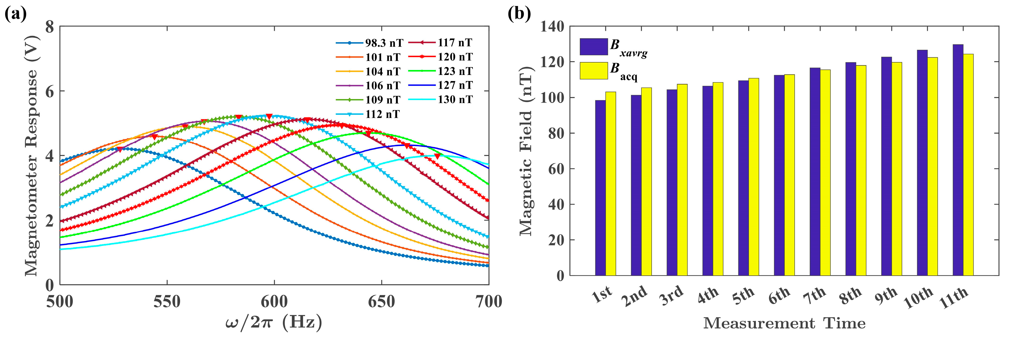
Two first-order resonance points, corresponding to with and with were extracted, averaged as , and plotted with the corresponding in Figure 3b, wherein the fit value was obtained based on the proportional relationship between and . In addition, the derived value of , which is called , was further calculated for each fit value of (the red solid line in Figure 3b). Then, we actively employed different magnetic field offsets along the same x-axis, each corresponding to . Simultaneously, we swept from 500 Hz to 700 Hz, with the same fixed modulated amplitude nT as that used when sweeping the magnetic field offset. The magnetometer response at each sweeping turn is recorded in Figure 4a, and its peak resonant frequency is marked with red inverted triangles.
The measurement results for different finite field offsets are summarized in Figure 4b. The represents the magnetic field acquired by detecting the resonance frequency , i.e., . The label of horizontal axis “Measurement Time” represents each measurement with different , as in Figure 4a, and “1st” and “11th” correspond to “= 98.3 nT” and “= 130 nT”, respectively. The was close to , i.e., within a 5% error range, which verified our non-zero finite measurement method based on the first-order resonance. In addition, the difference between and may result from the following factors: the residual magnetic field affected the detection of peaks when sweeping and caused the inequality between the actively applied magnetic field and ; the comprehensive effect of magnetic offset and modulated magnetic field induced the variation in the effective gyromagnetic ratio; and the nuclear slowing-down factor [30].
4.2. Spin Polarization Measurement
The spin polarization of 87Rb atoms was obtained by obtaining , which can be measured by determining the first-order resonance point. For instance, we swept the magnetic field offset along the x-axis with different values, ranging from 100 nT peak-peak value to 260 nT peak-peak value, with a fixed at 600 Hz. The magnetometer response for each sweep is plotted in Figure 5a. The first-order resonance points were extracted and recorded, and each corresponding slowing-down factor (spin polarization) was calculated and plotted in Figure 5b to present the relationship between the slowing-down factor (spin polarization) and . Increasing the modulated magnetic field amplitude leads to a larger relaxation rate .
By utilizing the spin polarization amplitude expression in Equation (13), we determined the relationship between and . The is composed of related to the modulation amplitude , and , which is not directly related to . Here, is the proportional factor of related to . For 87Rb atoms, according to Equation (13), can be expressed with respect to as follows:
The fit of the experimental data was performed according to Equation (14), and the results indicate that the coefficient of determination of the fit is 0.993. From Figure 5b, we observed that the larger the modulated magnetic field amplitude, the lower the spin polarization in the stable state. This finding is reasonable and consistent with the theories proposed by Shah et al. [31] and Yan et al. [32], for that the relaxation rate of alkali atoms caused by a modulated magnetic field is proportional to the squared value of the modulation amplitude.
4.3. In Situ Coil Constant Calibration
In the experiment, the actual value we set when applying a magnetic field was voltage , and the coil constant along the x-axis was In this equation, is the known resistor value, and the certain value of , i.e., , can be acquired through the resonance condition . The coil constant along the y-axis showed a similar relationship. However, simply utilizing the resonance condition to calibrate the coil constant may result in an error caused by the undetermined value of . Our method provides precise calibration based on combining the first-order resonance condition with the definitive value of obtained by fitting.
Deriving the relationship between and helps fitting for when , i.e., causes atoms unpumped with zero and definitive for 87Rb atoms. At the limit of , the magnetic field at the first-order resonance is known to be . In this manner, the coil constants can be precisely calibrated as .
We swept , from 200 Hz to 1000 Hz, with an invariable . The magnetometer response is illustrated in Figure 6a. At each sweeping turn, the pump light power was set as a different value ranging from 0.40 mW to 2.40 mW, with a step size of 0.20 mW, and the peak of each first-order resonance is marked in Figure 6a and recorded. The other experimental parameters were consistent with simulation parameters.
Subsequently, we listed the first-order resonance points (expressed as the modulation frequency ), and plotted Figure 6b to denote the relationship between and Determining the resonance in the modulation frequency is better than reading from the resonance when sweeping the magnetic field offset , due to the error caused by the residual magnetic fields.
Based on Equation (13), the relationship between and can be derived. is approximately proportional to , and . From the first-order resonance condition , the proportional relationship for is . Thereby, for 87Rb atoms the expression can be derived as
Equation (15) is adopted as the fit function between and .
We employed Equation (15) to fit the data in Figure 6b, and the fit value of for with can be obtained as Consequently, we showed that 14.54 nT/mA, and the coil constant along the same x-axis measured with a flux-gate magnetometer is 14.50 nT/mA, as shown in Figure 7a. This is regarded as the benchmark of the measured result of 𝑘𝑥 herein. The coil constants measured through these two methods, with a relative error of 0.29%, are almost similar. In addition, by employing a similar method, the coil constant along the y-axis was acquired as 14.53 nT/mA.
Furthermore, we evaluated the sensitivity of the magnetic field measurement based on the first-order resonance of a single-beam SERF magnetometer. The measurement sensitivity was analyzed by acquiring the noise spectrum of the output signal of the OPM. For direct measurement, a 100 pTrms magnetic calibration signal at 30.5 Hz and the magnetic field offset corresponding to the first-order resonance pointwere employed along the sensitive axis (x-axis in the experiment). Subsequently, the voltage output signal was acquired and collected for 60 s, and a noise spectral analysis was conducted to determine the sensitivities of the magnetometer. The sensitivity results are given in Figure 7b, where the maximum peaks in each noise spectrum represent the calibration signals. The sensitivity of magnetic field measurement was 54 fT/Hz1/2.
5. Conclusions
In this study, we assessed the nonzero-order parametric resonances of alkali-metal atoms in a single-beam SERF magnetometer and primarily focused on the first-order resonance. Based on the first-order resonance, not only can the nonzerofinite magnetic field be measured, but the spin polarization of alkali-metal atoms can also be determined by measuring the slowing-down factor. Moreover, precise calibration of the coil constants can be achieved by acquiring the first-order resonance points under a fitted equivalent zero light power (with a definitive for certain types of alkali-metal atoms). Our study summarizes parametric resonance, and the proposed method has the potential to function as a component of the systematic analysis of single-beam SERF magnetometers. Future studies may focus on the comprehensive response of SERF magnetometers at different harmonic and resonance orders.
Author Contributions
Conceptualization, K.W. and K.Z.; methodology, K.W.; software, N.X.; validation, K.W., X.L. and K.Z.; formal analysis, K.W.; investigation, Y.Y.; resources, K.Z.; data curation, K.W.; writing—original draft preparation, K.W.; writing—review and editing, K.Z.; visualization, K.W.; supervision, B.Z.; project administration, K.Z.; funding acquisition, B.Z. All authors have read and agreed to the published version of the manuscript.
Funding
This study was supported by the National Natural Science Foundation of China under Grant (No. 61903013).
Institutional Review Board Statement
Not applicable.
Informed Consent Statement
Not applicable.
Data Availability Statement
The data presented in this study are available upon reasonable request from the corresponding author.
Conflicts of Interest
The authors declare no conflict of interest.
References
- Kominis, I.K.; Kornack, T.W.; Allred, J.C.; Romalis, M.V. A subfemtotesla multichannel atomic magnetometer. Nature 2003, 422, 596–599. [Google Scholar] [CrossRef]
- Wakai, R.T. The atomic magnetometer: A new era in biomagnetism. AIP Conf. Proc. 2014, 1626, 46–54. [Google Scholar] [CrossRef] [Green Version]
- Boto, E.; Holmes, N.; Leggett, J.; Roberts, G.; Shah, V.; Meyer, S.S.; Muñoz, L.D.; Mullinger, K.J.; Tierney, T.M.; Bestmann, S.; et al. Moving magnetoencephalography towards real-world applications with a wearable system. Nature 2018, 555, 657–661. [Google Scholar] [CrossRef] [PubMed] [Green Version]
- Abel, C.; Afach, S.; Ayres, N.J.; Baker, C.A.; Ban, G.; Bison, G.; Bodek, K.; Bondar, V.; Burghoff, M.; Chanel, E.; et al. Measurement of the Permanent Electric Dipole Moment of the Neutron. Phys. Rev. Lett. 2020, 124, 081803. [Google Scholar] [CrossRef] [Green Version]
- Kim, Y.J.; Chu, P.-H.; Savukov, I.; Newman, S. Experimental limit on an exotic parity-odd spin- and velocity-dependent interaction using an optically polarized vapor. Nat. Commun. 2019, 10, 2245. [Google Scholar] [CrossRef] [PubMed] [Green Version]
- Dang, H.B.; Maloof, A.C.; Romalis, M.V. Ultrahigh sensitivity magnetic field and magnetization measurements with an atomic magnetometer. Appl. Phys. Lett. 2010, 97, 151110. [Google Scholar] [CrossRef] [Green Version]
- Higbie, J.M.; Rochester, S.M.; Patton, B.; Holzlöhner, R.; Calia, D.B.; Budker, D. Magnetometry with Mesospheric Sodium. Proc. Nat. Acad. Sci. USA 2011, 108, 3522–3525. [Google Scholar] [CrossRef] [Green Version]
- Iivanainen, J.; Zetter, R.; Parkkonen, L. Potential of on-scalp MEG: Robust detection of human visual gamma-band responses. Hum. Brain Mapp. 2020, 41, 150–161. [Google Scholar] [CrossRef] [PubMed] [Green Version]
- Boto, E.; Shah, V.; Hill, R.M.; Rhodes, N.; Osborne, J.; Doyle, C.; Holmes, N.; Rea, M.; Leggett, J.; Bowtell, R.; et al. Triaxial detection of the neuromagnetic field using optically-pumped magnetometry: Feasibility and application in children. NeuroImage 2022, 252, 119027. [Google Scholar] [CrossRef]
- Li, Z.; Wakai, R.T.; Walker, T.G. Parametric modulation of an atomic magnetometer. Appl. Phys. Lett. 2006, 89, 134105. [Google Scholar] [CrossRef] [Green Version]
- Hu, Y.; Hu, Z.; Liu, X.; Li, Y.; Zhang, J.; Yao, H.; Ding, M. Reduction of far off-resonance laser frequency drifts based on the second harmonic of electro-optic modulator detection in the optically pumped magnetometer. Appl. Opt. 2017, 56, 5927–5932. [Google Scholar] [CrossRef]
- Osborne, J.; Orton, J.; Alem, O.; Shah, V. Fully integrated, standalone zero field optically pumped magnetometer for biomagnetism. In Proceedings of the Proceedings SPIE 10548, Steep Dispersion Engineering and Opto-Atomic Precision Metrology XI; Shahriar, S.M., Scheuer, J., Eds.; SPIE: San Francisco, CA, USA, 2018; p. 10548. [Google Scholar] [CrossRef]
- Sheng, D.; Perry, A.R.; Krzyzewski, S.P.; Geller, S.; Kitching, J.; Knappe, S. A microfabricated optically-pumped magnetic gradiometer. Appl. Phys. Lett. 2017, 110, 031106. [Google Scholar] [CrossRef] [PubMed] [Green Version]
- Wang, J.; Fan, W.; Yin, K.; Yan, Y.; Zhou, B.; Song, X. Combined effect of pump-light intensity and modulation field on the performance of optically pumped magnetometers under zero-field parametric modulation. Phys. Rev. A 2020, 101, 053427. [Google Scholar] [CrossRef]
- Wang, K.; Zhang, K.; Zhou, B.; Lu, F.; Zhang, S.; Yan, Y.; Wang, W.; Lu, J. Triaxial closed-loop measurement based on a single-beam zero-field optically pumped magnetometer. Front. Phys. 2022, 10, 1059487. [Google Scholar] [CrossRef]
- Cohen-Tannoudji, C.; Dupont-Roc, J.; Haroche, S.; Laloë, F. Diverses résonances de croisement de niveaux sur des atomes pompés optiquement en champ nul. I. Théorie. Rev. Phys. Appl. (Paris) 1970, 5, 95–101. [Google Scholar] [CrossRef]
- Slocum, R.E.; Marton, B.I. Measurement of Weak Magnetic Fields Using Zero-Field Parametric Resonance in Optically Pumped He4. IEEE Trans. Magn. 1973, 9, 221–226. [Google Scholar] [CrossRef]
- Xiao, W.; Wang, H.; Zhang, X.; Wu, Y.; Wu, T.; Chen, J.; Peng, X.; Guo, H. In Situ Calibration of Magnetic Field Coils Using Parametric Resonance in Optically-pumped Magnetometers. In Proceedings of the 2021 Joint Conference of the European Frequency and Time Forum and IEEE International Frequency Control Symposium (EFTF/IFCS), Gainesville, FL, USA, 7–17 July 2021; pp. 1–3. [Google Scholar] [CrossRef]
- Eklund, E.J. Microgyroscope Based on Spin-Polarized Nuclei. PhD Thesis, University of California, Irvine, CA, USA, 2008. [Google Scholar]
- Chen, C.; Jiang, Q.; Wang, Z.; Zhang, Y.; Luo, H.; Yang, K. A non-interference method for measurement of transverse relaxation time of the alkali metal magnetometer in nuclear magnetic resonance oscillator. AIP Adv. 2020, 10, 065303. [Google Scholar] [CrossRef]
- Jiang, Q.; Luo, H.; Zhan, X.; Zhang, Y.; Yang, K.; Wang, Z. Avoiding the impact of the heater-induced longitudinal field on atomic magnetometers. J. Appl. Phys. 2018, 124, 244501. [Google Scholar] [CrossRef]
- Yang, H.; Wang, Q.; Zhao, B.; Li, L.; Zhai, Y.; Han, B.; Tang, F. Magnetic field sensing based on multi-order resonances of atomic spins. Opt. Express 2022, 30, 6618. [Google Scholar] [CrossRef]
- Ledbetter, M.P.; Savukov, I.M.; Acosta, V.M.; Budker, D.; Romalis, M.V. Spin-exchange-relaxation-free magnetometry with Cs vapor. Phys. Rev. A 2008, 77, 033408. [Google Scholar] [CrossRef] [Green Version]
- Appelt, S.; Baranga, A.B.-A.; Erickson, C.J.; Romalis, M.V.; Young, A.R.; Happer, W. Theory of spin-exchange optical pumping of 3He and 129Xe. Phys. Rev. A 1998, 58, 1412–1439. [Google Scholar] [CrossRef] [Green Version]
- Dong, H.F.; Fang, J.C.; Zhou, B.Q.; Tang, X.B.; Qin, J. Three-dimensional atomic magnetometry. Eur. Phys. J. Appl. Phys. 2012, 57, 21004. [Google Scholar] [CrossRef]
- Seltzer, S.J. Developments in Alkali-Metal Atomic Magnetometry. PhD Thesis, Princeton University, Princeton, NJ, USA, 2008. [Google Scholar]
- Chen, Y.; Zhao, L.; Zhang, N.; Yu, M.; Ma, Y.; Han, X.; Zhao, M.; Lin, Q.; Yang, P.; Jiang, Z. Single beam Cs-Ne SERF atomic magnetometer with the laser power differential method. Opt. Express 2022, 30, 16541. [Google Scholar] [CrossRef] [PubMed]
- Wu, W.; Zhou, B.; Liu, G.; Chen, L.; Wang, J.; Fang, J. Novel nested saddle coils used in miniature atomic sensors. AIP Adv. 2018, 8, 075126. [Google Scholar] [CrossRef] [Green Version]
- Wang, J.; Zhou, B.; Wu, W.; Chen, L.; Fang, J. Uniform Field Coil Design Based on the Target-Field Method in Miniature Atomic Sensors. IEEE Sens. J. 2019, 19, 2895–2901. [Google Scholar] [CrossRef]
- Xiao, W.; Wu, T.; Peng, X.; Guo, H. Atomic spin-exchange collisions in magnetic fields. Phys. Rev. A 2021, 103, 043116. [Google Scholar] [CrossRef]
- Shah, V.; Romalis, M.V. Spin-Exchange-Relaxation-Free Magnetometry Using Elliptically-Polarized Light. Phys. Rev. A 2009, 80, 013416. [Google Scholar] [CrossRef] [Green Version]
- Yan, Y.; Lu, J.; Zhang, S.; Lu, F.; Yin, K.; Wang, K.; Zhou, B.; Liu, G. Three-axis closed-loop optically pumped magnetometer operated in the SERF regime. Opt. Express 2022, 30, 18300. [Google Scholar] [CrossRef] [PubMed]
Figure 1.
(a) Schematic of our single-beam SERF magnetometer with the modulated magnetic field along the x-axis. (b) Simulation results of the magnetometer response under different and , with nT.
Figure 1.
(a) Schematic of our single-beam SERF magnetometer with the modulated magnetic field along the x-axis. (b) Simulation results of the magnetometer response under different and , with nT.

Figure 2.
Experimental setup. PMF: polarization maintaining fiber; C: collimating lens; LP: linear polarizer; QP: quarter-wave plate; PD: photodiode; TIA: transimpedance amplifier; LIA: lock-in amplifiers; DAQ: data-acquisition; R1, R2, and R3: resistors.
Figure 2.
Experimental setup. PMF: polarization maintaining fiber; C: collimating lens; LP: linear polarizer; QP: quarter-wave plate; PD: photodiode; TIA: transimpedance amplifier; LIA: lock-in amplifiers; DAQ: data-acquisition; R1, R2, and R3: resistors.

Figure 3.
(a) Magnetometer responses when sweeping the magnetic field offset under different modulated magnetic field frequencies ranging from 500 Hz to 700 Hz. Each peak of at the first-order resonance is marked with a red inverted triangle and recorded. (b) Each first-order resonance point (red solid circle) with different modulated magnetic frequencies . The fit value is presented as a red solid line.

Figure 4.
(a) Dependence of the magnetometer response on under different magnetic field offsets . Resonance frequency peaks are marked with red inverted triangles. (b) Comparison between the active applied magnetic field and acquired from (a). The label of horizontal axis “Measurement Time” represents each measurement with different .

Figure 5.
(a) Magnetometer response when sweeping the magnetic field offset along the x-axis with different values ranging from 260 nT peak-peak value to 460 nT peak-peak value, and the fixed at 600 Hz. The peak of each first-order resonance is marked with red inverted triangles and recorded. (b) The slowing-down factor and spin polarization when different values are employed, wherein each record is extracted from the data depicted in subfigure (a). The solid circle points represent the experimental data, whereas each solid curve represents the fit curve according to Equation (14).

Figure 6.
(a) Magnetometer response to different frequencies of the modulated magnetic field and with different pump light powers (plotted using different colors). Each peak of magnetometer response of at the first-order resonance is marked with a red inverted triangle and recorded. (b) The plotted under different , wherein each record is extracted from the data depicted in (a). This plot indicates the relationship between and , and, moreover, the fit value of for can be acquired.

Figure 7.
(a) The measurement of magnetic field generated by the same coil as that in Section 4.3 with different coil currents, and using a flux-gate magnetometer, for comparison. (b) Sensitivity of the magnetic field measurement based on the first-order resonance of single-beam SERF magnetometers. The measurement sensitivity is evaluated by applying the calibration magnetic field signal to the magnetometer along with the modulated magnetic field. The sensitivity of magnetic field measurement is 54 fT/Hz1/2.

Disclaimer/Publisher’s Note: The statements, opinions and data contained in all publications are solely those of the individual author(s) and contributor(s) and not of MDPI and/or the editor(s). MDPI and/or the editor(s) disclaim responsibility for any injury to people or property resulting from any ideas, methods, instructions or products referred to in the content. |
© 2023 by the authors. Licensee MDPI, Basel, Switzerland. This article is an open access article distributed under the terms and conditions of the Creative Commons Attribution (CC BY) license (https://creativecommons.org/licenses/by/4.0/).
Share and Cite
MDPI and ACS Style
Wang, K.; Zhang, K.; Xu, N.; Yan, Y.; Li, X.; Zhou, B. Nonzero-Order Resonances in Single-Beam Spin-Exchange Relaxation-Free Magnetometers. Photonics 2023, 10, 458. https://doi.org/10.3390/photonics10040458
AMA Style
Wang K, Zhang K, Xu N, Yan Y, Li X, Zhou B. Nonzero-Order Resonances in Single-Beam Spin-Exchange Relaxation-Free Magnetometers. Photonics. 2023; 10(4):458. https://doi.org/10.3390/photonics10040458
Chicago/Turabian StyleWang, Kun, Kaixuan Zhang, Nuozhou Xu, Yifan Yan, Xiaoyu Li, and Binquan Zhou. 2023. "Nonzero-Order Resonances in Single-Beam Spin-Exchange Relaxation-Free Magnetometers" Photonics 10, no. 4: 458. https://doi.org/10.3390/photonics10040458
Note that from the first issue of 2016, this journal uses article numbers instead of page numbers. See further details here.