The Optical Inverse Problem in Quantitative Photoacoustic Tomography: A Review

Department of Instrument Science and Engineering, Shanghai Jiao Tong University, Shanghai 200240, China
*
Author to whom correspondence should be addressed.
Photonics 2023, 10(5), 487; https://doi.org/10.3390/photonics10050487
Submission received: 27 March 2023
/
Revised: 16 April 2023
/
Accepted: 19 April 2023
/
Published: 24 April 2023
(This article belongs to the Special Issue Photoacoustic Imaging: Applications, Approaches, and Systems)
Abstract
:Photoacoustic tomography is a fast-growing biomedical imaging modality that combines rich optical contrast with a high acoustic resolution, at depths in tissues. Building upon the foundation of this technique, novel quantitative photoacoustic tomography fully leverages its advantages while further delivering improved quantification capabilities to produce high-accuracy concentration estimates, which has attracted substantial research interest in recent years. The kernel challenge associated with quantitative photoacoustic tomography is an optical inverse problem aiming to recover the absorption coefficient distribution from the conventional photoacoustic image. Although the crucial importance of the optical inversion has been widely acknowledged, achieving it has remained a persistent challenge due to the inherent non-linearity and non-uniqueness. In the past decade, numerous methods were proposed and have made noticeable progress in addressing this concern. Nevertheless, a review has been conspicuously absent for a long time. Aiming to bridge this gap, the present study comprehensively investigates the recent research in this field, and methods identified with significant value are introduced in this paper. Moreover, all included methods are systematically classified based on their underlying principles. Finally, we summarize each category and highlight its remaining challenges and potential future research directions.
1. Introduction
A major current focus in functional imaging is to estimate distributions of molecular concentrations and related quantities, which serve as biomarkers for some diseases and complement structural imaging techniques, enabling a more comprehensive understanding of internal tissue states with significant medical value [1,2,3,4,5,6,7]. As an illustration, blood oxygen saturation is a pivotal factor in tumor progression, which is derived from the concentrations of oxygenated and deoxygenated hemoglobin. As for a rapidly growing tumor, an elevated rate of oxygen consumption may lead to a reduction in oxygen supply, particularly in the central region where hypoxia possibly occurs. This highlights the importance of quantifying blood oxygen saturation levels and their relationship with tumor growth, which may offer insights into therapeutic interventions for cancer treatments [8,9,10]. Photoacoustic tomography (PAT) is a rapidly growing and promising biomedical imaging modality utilizing the photoacoustic (PA) effect [11]. Benefiting from the optical absorption measurement mechanism, it is intrinsically sensitive to molecular information and can produce images with rich optical contrast. Meanwhile, the use of acoustic detection enables PAT to achieve greater resolution and imaging depth compared to traditional purely optical imaging techniques, attributed to the low scattering and attenuation of sound waves in biological media [12,13,14]. Furthermore, PAT is envisioned to be a universal imaging modality since it is theoretically capable of imaging any light-absorbing material, including both endogenous chromophores, such as hemoglobin, and exogenous contrast agents such as nanomaterials [15,16,17].
However, conventional schemes that utilize PAT and linear spectral unmixing have been found to yield unsatisfactory results in estimating molecular concentrations due to the significant impact of spatially varying and wavelength-dependent fluence within the illuminated volume, namely spectral coloring [18,19,20,21]. Quantitative photoacoustic tomography (qPAT) is a novel imaging technique that has attracted substantial research interest in recent years. Building upon the foundation of PAT, qPAT not only inherits its advantages but also provides enhanced quantification capabilities to produce high-accuracy concentration estimates [21,22,23]. In contrast with conventional schemes that directly estimate chromophore concentrations from PA images via spectral unmixing, qPAT takes advantage of an additional intermediate step, an optical inversion, to retrieve absorption coefficient distributions from PA images. Then, the resultant distributions are used to conduct spectral unmixing, just as illustrated in Figure 1. Theoretical details for the conventional schemes are presented in Section 2.2. Due to this process, qPAT effectively overcomes the undesirable effect of fluence, corrects the distorted spectral profiles associated with each pixel from measurements, and ultimately contributes to highly accurate concentration estimates.
In most previous research, qPAT has been commonly considered to contain two inverse problems (optical and acoustic), from the measured acoustic time series to the chromophore concentration distributions [22,24,25,26]. In contrast, the present paper further divides the previous optical portion into a more specific optical inverse problem and a spectroscopic inverse problem, as shown in Figure 1. In this manner, we can give full prominence to the unsolved challenge, the newly defined optical inverse problem that is dedicated to recovering absorption coefficient distributions from measured PA images or more commonly absorbed energy density distributions (assuming a negligible Grüneisen parameter), given that the acoustic and spectroscopic inversions have been properly addressed by the well-established PAT and spectral unmixing techniques beyond the scope of this study [20,27]. The difficulties associated with the optical inverse problem arise from the following two major aspects. First, optical inversion is highly nonlinear, since the initial pressure rise in each pixel is linearly dependent on the product of the absorption coefficient and the received fluence, while the local fluence is in turn intricately linked to the absorption coefficient distribution of the entire volume. On the other hand, the non-uniqueness imposes intractability as well, leading to the result that tissues with distinct optical properties may lead to the same fluence map due to the highly stochastic nature of optical interactions.
Over the past decade, significant advancements have been made in resolving the optical inverse problem. This study endeavors to conduct a comprehensive investigation of the recent progress, including modifications and enhancements for canonical frameworks, as well as newly developed methods. Among them, according to their feasibility, applicability, and potential for further developments, the paper includes methods with considerable value with necessary contexts and theoretical explanations. Notably, not all invasive approaches are within the scope of this study, such as methods requiring intravenous injection or substance insertion. All included methods are systematically classified based on their underlying principles, as shown in Figure 2. The rest of this paper is organized as follows: Section 2 first provides a concise introduction to fundamentals. Section 3 offers an overview of all the methods studied. Conclusive remarks on each category, as well as their remaining challenges and future directions for research, are presented in Section 4.
2. Theoretical Fundamentals
2.1. Generation of Initial Pressure Rise
In a PA process, short pulses of light are used to irradiate media, resulting in the absorption of photon energy and subsequently heating, thereby inducing local thermoelastic expansion. This expansion, in turn, converts the temperature increase to a corresponding initial pressure rise. If the excitation light pulse width satisfies both the pressure and thermal constraints, the initial pressure rise (Pa) is directly proportional to the temperature increase T (K):
where denotes the thermal coefficient of volume expansion (K), and denotes the isothermal compressibility (Pa−1). Combined with the photothermal conversion, the above equation can be rewritten as [11,28]:
where represents optical absorption coefficient (cm−1), and is local optical fluence (J· cm−2). H is the absorbed energy density, derived from the product of the fluence and the absorption coefficient. is the Grüneisen parameter (dimensionless) and denotes the efficiency (dimensionless) of converting light into heat energy, both of which are nearly uniformly distributed within biological media. Hence, for simplicity, a common assumption is that the energy density obtained by photon absorption is considered equivalent to the initial pressure and then used as initial data for the optical inversion, which implies the parameters are negligible. This assumption is widely adopted in the later-mentioned studies. Notably, it is found in Equation (2) that is not only determined by but also depends on , which provides a theoretical insight for the spectral coloring problem mentioned in the next section.
2.2. Photoacoustic Tomography-Based Concentration Measurement
Photoacoustic tomography utilizes ultrasonic transducers positioned outside the medium to capture broadband ultrasound waves generated by the PA effect and record them as time series signals, namely PA signals. The PA image is subsequently formed from the measured data via a reconstruction algorithm for photoacoustic computed tomography (PACT), or a focused-scanning scheme in the case of photoacoustic microscopy (PAM) [13,29]. The pixel values of the PA image serve as a measure of the initial pressure rises.
For quantitative measurement tasks that are based on PAT, it is necessary to obtain a collection of multispectral PA images by illuminating media with light of different wavelengths. In this manner, the spectral profile of the local initial pressure rise is resolved in each pixel [30,31,32,33]. The fundamental assumption underlying this scheme is that fluence is uniformly distributed within media, hence that, in each pixel, local initial pressure rises are directly proportional to respective absorption coefficients. Subsequently, a linear mixture model of spectra can be adopted, wherein the measured pressure spectrum is proportional to the weighted sum of molar absorption spectra of constituent chromophores and the associated weights represent the constituent concentrations [23], as shown in the following formula:
where and denote the measured initial pressure rise and the absorption coefficient, respectively, at point and wavelength . For each of N individual components, and denote the molar absorption coefficient at wavelength and the local concentration at point , respectively. Then, if the molar absorption spectra of all components are given, the concentrations of each chromophore in a single pixel would be readily resolved via a linear regression algorithm [16,34]. This procedure is commonly referred to as linear spectral unmixing. From the mathematical perspective, the above PAT-based scheme is constituted by an acoustic inverse problem and a spectroscopic inverse problem.
2.3. Spectral Coloring
In Section 2.2, the initial pressure, or absorbed energy density, is assumed to be proportional to the absorption coefficient. However, this assumption can hardly hold in real scenarios, particularly for imaging regions that are located deep [19,20,21]. The incident light undergoes wavelength-dependent absorption and scattering as it propagates through media, leading to the accordingly wavelength-dependent and spatially varying fluence. Thus, the fluence cannot be simply assumed to have a uniform impact throughout the entire region of interest [21,35]. Numerous studies have revealed that the measured initial pressure spectrum extracted from a set of multispectral PA images differed dramatically from the expected absorption spectrum due to the distortion by the unknown fluence spectrum, a phenomenon known as spectral coloring [19,22,36]. The spectral coloring results in unacceptable concentration estimates, seriously hindering quantitative applications of PAT.
The phenomenon of spectral coloring has been acknowledged as the most critical challenge in PA-based quantitative measurements, attracting considerable attention in recent times [20,22,36]. To address the impact of spectral coloring, it is necessary to eliminate the fluence-related component from the measured data, namely recovering absorption property distributions, which is precisely the essence of the optical inverse problem investigated in this paper.
3. Methods for the Optical Inverse Problem
3.1. Forward Model-Based Methods
Forward model-based methods are based on a forward model that mathematically describes the physical mechanism of data acquisition to address the optical inverse problem. The complete schematic diagram of forward modeling is illustrated in Figure 3. Notably, it is not essential to simulate the entire process for methods presented in this section, but the light propagation model must be entailed. As shown in Equation (2), if the fluence distribution is known, all other relevant variables are easily determined. Therefore, the crucial factor of all forward operators is the process for simulating light propagation in biological media, where both absorption and scattering play an important part.
Several commonly adopted models for light propagation are outlined in the following. The first thing to note is that, for any model here, it is necessary to specify the geometries and optical properties (including absorption, scattering, anisotropy, and refractive index) of the simulated medium along with the used illumination conditions in advance. The radiative transfer equation (RTE) is a widely accepted model that accurately describes light propagation by utilizing energy conservation within a localized volume. Nevertheless, the RTE is an integrodifferential equation expressed in terms of radiance, which is typically not available to obtain the analytic solution. Due to the radiance’s angular dependence, both angular and spatial discretization are required for the numerical solution, resulting in a computationally intensive process [11,37]. An established strategy to mitigate the computational complexity associated with the RTE is to leverage assumptions that simplify its expression. Among them, the diffusion approximation (DA) model is an extensively adopted one, which assumes radiance is weakly anisotropic in strongly scattering media and can be expressed via only the first two order spherical harmonics, leading to a diffusion equation in terms of fluence with high computational efficiency [11]. However, the DA is not valid in proximity to sources and boundaries. To overcome this limitation, the delta-Eddington model (delta-E) represents the fluence as the sum of collimated fluence and diffuse fluence, thus compensating for forward-peaked scattering by introducing a delta term in the phase function [38,39]. This enhancement extends the applicability of the delta-E model to regions where the DA fails while maintaining comparable computational efficiency. In contrast to the above models that are formulated explicitly, the Monte Carlo (MC) model operates as a stochastic approach that employs a random walk algorithm of photon packages, each with an initial weight, to generate fluence maps. This methodology is widely considered to be the gold standard, delivering exceptional accuracy when a sufficiently large number of photon packages are simulated [40]. Nevertheless, the MC model remains computationally demanding, and it offers limited mathematical insights. It is worth noting that within a given forward model-based framework, all those light propagation models are available, despite featuring varying accuracy and computational efficiency. As such, researchers must carefully navigate the trade-off between these factors to select an appropriate model that aligns with the specific requirements of the problem to be solved. The remainder of this section shall organize forward model-based methods into four distinct subcategories according to different implementation frameworks, as concluded in Table 1.
3.1.1. Fluence Correction Based on Prior Knowledge
Upon a cursory examination of Equation (2), one may observe that if the fluence distribution is known, the optical inverse problem can be resolved via dividing the PA image by the fluence pixel-by-pixel; this process is termed fluence correction [41]. Based on this framework, optical properties are predefined as prior knowledge typically obtained from previous literature, experience, and measured data, to produce fluence distributions. This framework only requires modeling light propagation a single time with small computational efforts, but its efficacy heavily relies on the quality of the prior information. In the simplest case, optical properties are assumed to be homogeneous throughout the region of interest, by which light propagation models are easy to implement for estimating fluence distributions and then recover the absorption distribution by fluence correction, such as 1-D exponential decay models [42,43], the DA [44], and the MC [9,45].
However, the above studies overlook the optical inhomogeneity in media, which is particularly evident on surfaces and internal tissue boundaries where sharp discontinuities in terms of optical properties occur. To achieve a high-accuracy fluence distribution estimate, it is imperative to take more internal structure details within regions of interest into consideration. Thanks to structural refinements, the assignments of optical properties are more realistic. Deng et al. [46] constructed the finger-joint skin as a two-layer model with epidermis and dermis; Zhao et al. [47] divided the illuminated breast tissue into a skin layer and a breast adipose layer; Tang and Yao [48] simulated the fluence distribution with a mouse brain model that was labeled with abundant tissue types and related optical properties. In addition, complementary structural modalities (e.g., ultrasound (US) imaging) can provide more insights into anatomical information. Han et al. [49] manually segmented the object’s boundary and internal tissues via the co-registered US images under the guidance of experienced physicians. Moreover, segmentation algorithms were applicable as well. Pattyn et al. [50] adopted the seeded region growing method on the US image to automatically identify the boundary and partition involved tissues. Mandal et al. and Liang et al. utilized an active contour model [51] and a three-dimensional (3-D) optimal graph search algorithm [45], respectively, to identify the unsmooth surfaces of objects from backgrounds.
3.1.2. Model Fitting Methods
The second subclass of methods is to fit data from multiple measurements to a specified forward operator. Based on the optical homogeneity assumption of media, Held et al. [52] irradiated the sample at multiple locations to acquire a set of data. They approximated the medium as a semi-infinite 3-D geometry and adopted the DA model to simulate light propagation. In this manner, the effective attenuation coefficient fully determined the fluence distribution. The fluence received at a specific point within the illumination volume varied with the illumination location, owing to the distinctive distances between the source and detection points. The effective attenuation coefficient was obtained from the constructed characteristic curve of measured data and corresponding distances. Subsequently, the DA model was able to generate the fluence map and the desired absorption coefficient was ultimately retrieved by fluence correction. Similar frameworks have been explored in other literature as well [23,53].
3.1.3. Fixed-Point Iteration Methods
The third subcategory pertains to an iterative calculation of the absorption coefficient map from measured data through a fixed-point iteration algorithm. Under this framework, the absorbed energy density distribution is treated as the original data from measurements and used as the starting point of algorithms. Cox et al. [54] proposed the first fixed-point iteration algorithm in this field, which approached the recovery of absorption coefficients as a nonlinear equation-solving problem, as formulated in Equation (4) for each pixel:
where is the absorbed energy density at from the measurement. In the k-th iteration, if the residual between the simulated and measured absorbed energy density failed to satisfy the prescribed error tolerance, the absorption coefficients were recalculated by Equation (5), then the was obtained from the delta-E model.
Based on this framework, Liu et al. [55] took advantage of the MC model to improve the accuracy of the and Zhang et al. [56] recently adopted the DA model to achieve high efficiency.
Additionally, Zhang et al. [57] utilized internal structure contours provided by high-contrast Magnetic Resonance Imaging (MRI) to achieve organ-level segmentation within the sample. Assuming uniform absorption distribution within each region, the unknowns were significantly reduced, resulting in diminished computational complexity and fast convergence.
Wu et al. [58] proposed a novel algorithm that involved implementing spectroscopic inversion to derive constituent concentrations following the calculation of the . Notably, the scattering coefficient map and anisotropy map were iteratively updated based on the assumed linear relationships with the constituent concentrations. Therefore, the algorithm to some extent extends the potential applicability of this framework to scenarios where the scattering coefficient and anisotropy coefficient are not available.
3.1.4. Minimization-Based Methods
Each of the mentioned methods imposes certain limitations, such as the need for prior knowledge or optical homogeneity assumptions, which can be challenging to fulfill under real measurement scenarios, therefore constraining the potential for high-accuracy applications. To overcome all above limitations, one effective approach is to solve the optical inverse problem within an optimization framework, where optical properties (typically absorption and scattering coefficients) are iteratively updated and fed into a forward model to generate simulated data. The iteration process continues until a defined objective function that evaluates the difference between the simulated data and the data obtained experimentally by PAT is minimized. The underlying principle is that, as the difference decreases, the updated parameters ultimately converge to the actual values. The framework has demonstrated the ability to handle media with arbitrary inhomogeneities, even in the absence of significant prior knowledge of the optical properties. Nevertheless, it necessitates increased computational complexity and longer computation time, relative to single modeling methods. As the assumption mentioned in Section 2.1, the measured data conventionally represent the absorbed light energy density distribution within this framework, assuming that the uniform Grüneisen coefficient has been normalized.
In a pioneering study, Cox et al. [59] proposed an optimization framework, as illustrated in Figure 4, to estimate the absorption and reduced scattering coefficients concurrently from the absorbed energy distribution . In each iteration, the simulated absorbed energy density was calculated by forward modeling based on the delta-E model. The objective function was formulated as the sum of squared differences between and within all pixels, which was iteratively minimized until it converged to the minimal.
To the present day, this minimization-based framework has continued to be utilized as a basis for subsequent research endeavors. Approaches developed to facilitate and enhance this framework are concluded in the rest of this section.
(i) Research for implementing the minimization framework. To perform the forward model-based minimization, optimization algorithms play a key role within the framework, as illustrated in Figure 4, which offers the update vector of iterative variables. Two types of algorithms that merit mention are the gradient-based and Jacobian-based approaches. The former primarily refers to the limited-memory Broyden–Fletcher–Goldfarb–Shanno algorithm (L-BFGS) [25,59,60,61,62], which is a quasi-Newton method. Quasi-Newton methods aim to provide a super-linear convergence speed close to Newton’s method with less computational effort by using the secant method to approximately update the Hessian matrix, instead of calculating it from scratch [63]. On this basis, the popular L-BFGS further utilizes gradient vectors of successive iteration points to directly update the inverse of the Hessian matrix in a two-loop recursion manner, which, hence, is less computationally intensive and highly memory-efficient due to only necessitating the calculation and storage of gradients, especially for large-scale problems. On the other hand, the Jacobian-based optimization strategy pertains primarily to the Gauss–Newton method [26,64,65], which requires the explicit computation and storage of the Jacobian matrix. Although this approach is more storage-intensive, it has fewer computation processes when compared to gradient-based methods.
Once the optimization algorithm is determined, the next issue requiring significant concern is to obtain the derivatives of the objective function with respect to optical properties. Based on the perturbation theory, the variation in local absorbed energy caused by variations in optical properties is contributed by two components, as formulated in the following:
where and denote the absorption coefficient and fluence in the initial state, and hat symbols are used to mark their perturbations. The first term is simple to solve, but the second is intractable on account of the highly nonlinear relation of the fluence with optical properties. To acquire the desired derivative, the underlying relationship between perturbed optical properties and resultant changes in fluence must be established.
The methods employed to address the second term can be categorized into two groups. Given an explicit form model, a well-established assumption is that the model retains good validity for the perturbation state, which only considers the linear variations in involved variables [24,66]. Therefore, the so-called sensitivity equations can be constructed [22], revealing the required relationship to calculate the second term. Presenting the case of the DA model for a simple explanation [25,67], the perturbed fluence distribution, induced by small variations in the local optical properties at a given point , is governed by the equations
where is the diffusion coefficient of the initial state and its small variation is indicated by a hat symbol. is a Dirac delta function. Detail implementations can be found in the following works of literature [59,61,62]. It is noteworthy that the utilization of the adjoint operator theory is a common approach to attain superior computational efficiency in resolving such perturbation state equations [24,25,59,60,61,62].
In contrast with explicit models, the Monte Carlo (MC) simulation presents a greater challenge in the computation of derivatives, owing to the limited mathematical insight it offers. Hochuli et al. [68] proposed a radiance MC (RMC) algorithm that assumed the angle-dependent radiance could be effectively expressed by a few orders of a harmonic angular basis and provided a way to produce an analytical solution of the radiance in an MC simulation manner. In this context, the MC simulation worked as the RTE; hence, its derivative was able to be solved via a method for the RTE [61]. This algorithm has been applied in several later studies and demonstrated considerable feasibility [69,70,71,72]. Additionally, Leino et al. [73] proposed an alternative algorithm that revitalized the previously developed perturbation MC (PMC) method by Hayakawa et al. [74]. During the MC simulation, all simulated trajectories were recorded to approximate the overall trajectory space. As the radiance of each trajectory was expressed by the incidence intensity and a series of exponential decay functions associated with traveling movements, its derivative with respect to the local absorption and scattering of each passing region was easily computed. Performing this computation over the recorded space, the derivative of fluence was subsequently obtained by summing up the radiance derivatives for each trajectory.
(ii) Research for enhancements for the minimization framework. While the minimization framework can be conducted based on the above approaches theoretically, a successful optical inversion with desired results demands further research. One of the most significant obstacles is the non-uniqueness problem that arises from the highly stochastic nature of optical interactions. Hence, tissues with distinct optical properties might result in the same simulated distribution, leading to the possibility of converging to a wrong solution. A commonly adopted strategy for addressing the non-uniqueness is to incorporate a regularization term into the objective function. Tikhonov regularization is frequently employed to achieve solutions with desirable smoothness properties [75]. Alternatively, total variation regularization has been demonstrated to effectively remove false details while preserving sharp contrast at tissue edges or boundaries, making it particularly suited for the piece-wise constant characteristic of biological tissues [22,76,77]. Some more efforts have been made for the improved performance of total variation by featuring it with directional sensitivity [78,79,80], which mitigates the excessive smoothness and recovers directional textures.
Moreover, the utilization of multiple illumination sensing has proven the ability to alleviate the non-uniqueness. It is postulated that measurements obtained from multiple light source positions can impart a unique contribution to the desired optical property distributions [81,82,83,84,85,86]. The optimization algorithm considers the measured data from multiple illuminations, resulting in an overdetermined condition where all independent measurements constrain the optimization process to converge in the right direction. In addition, analyzing measured data from multiple wavelengths delivers comparable effectiveness in addressing the non-uniqueness [21,87,88,89]. In this context, the entire multispectral images are concurrently processed, allowing for the direct estimation of local concentrations of chromophores by solving both the optical and spectroscopic inverse problems together. In that case, if the number of employed wavelengths surpasses the number of unknown concentrations, an overdetermined condition is achieved as well, to pose further constraints on the convergence process.
Furthermore, incorporating additional information from complementary measurements demonstrates the capability in reducing solution space. Based on the standard framework, Nykänen et al. [90] coupled the measured diffuse light emanating from the surface by integrating its difference with data from forward modeling into the objective function, resulting in a joint minimization problem that effectively alleviated the non-uniqueness and produced improved estimates.
Apart from the non-uniqueness issue, imperfect measurement data also cause a considerable issue, which is generally induced by system noise, limited detections, and reconstruction errors [91,92,93,94]. Since the optimization process is governed by minimizing the difference between the measured and simulated data, the presence of inherent measured noise and artifacts may propagate to results, leading to decreased accuracy. Tarvainen et al. [26,64] proposed a Bayesian framework that treated all input and output parameters as random variables following a Gaussian distribution with specified means and variances. The estimation of optical properties was carried out by the mean of statistical inference complying with the maximum posterior (MAP) estimation. The Bayesian framework has been demonstrated in several studies to effectively account for measurement imperfections, mitigating error propagation and resulting in a more accurate estimate [95,96,97].
Moreover, Naser et al. [89] proposed a method for generating a signal-to-noise ratio (SNR) map based on a large dataset of background noise acquired under non-irradiation conditions, which was utilized to evaluate the noise level of individual pixels. An optimal threshold was then determined and employed to exclude highly noise-corrupted data from the minimization process. Kim et al. [83] adopted the sum of intensities in each pixel obtained from multiple measurements with varying light source configurations as an indicator for the signal-to-noise ratio (SNR). The SNR map was incorporated into the objective function as a pixel-wise weighting factor for the squared difference, thus assigning greater importance to pixels with higher SNR values.
It is noteworthy that, from a mathematical viewpoint, both the Bayesian-based and SNR-based methods can be classified as variants of regularization. Hence, it follows logically that other regularization techniques may also enable enhanced robustness to measured errors.
In addition, some researchers have attempted to solve the acoustic and optical inverse problems of qPAT together as a joint problem to alleviate the impact of measured data errors [25,93,98,99,100]. The results of the optical forward operator were directly coupled with the acoustic forward operator as input data and the value that needed minimizing was the difference between the results from the acoustic forward operator and the raw time series pressure recorded by ultrasonic detectors. In this context, the error-containing images were no longer unchanged, as in the methods mentioned earlier, but were modified iteratively to achieve the optimal solution from a global perspective of the measurement process. It turned out that the direct scheme yielded superior results with better stability.
3.2. Fluence Correction with Assisted Techniques
The second category of methods is to measure fluence distributions through complementary techniques, after which absorption coefficient distributions are straightforwardly derived via fluence correction, as mentioned in Section 3.1.1.
3.2.1. Fluence Correction with Diffusion-Based Techniques
Methods described in this section are founded upon the diffusion theory. Early efforts in this field, as demonstrated by Yin et al. [101,102], involved the adoption of photodetectors to measure the emergent flux, which was utilized to derive the fluence map through model-based diffuse optical tomography (DOT). Subsequently, the absorption distribution was recovered by normalizing the raw PA image with the resultant fluence map. Preliminary validation experiments conducted on simple geometric phantoms yielded promising results, with notable reductions in quantitative errors induced by the non-uniform fluence.
Recently, Ulrich et al. [103] adopted frequency-domain DOT using intensity-modulated excitation light with a sinusoidal profile. They collected time-dependent optical signals detected across surfaces and retrieved optical properties by employing a reconstruction algorithm based on the time-dependent diffusion approximation (DA) model. Lastly, the resultant properties were fed into the DA model to generate the fluence map.
Moreover, Mahmoodkalayeh et al. [104] proposed a mutual compensation method, named the PAT-guided-DOT-compensated-PAT (PAT-DOT-PAT) scheme. The scheme leveraged structural information from the initial PA image to guide the DOT and then the DOT would generate fluence maps with higher resolution and finer spatial details. Simulation results indicated that the PAT-DOT-PAT approach outperformed previous DOT-compensated PAT methods in terms of estimating optical properties, leading to an improved fluence estimate.
3.2.2. Fluence Correction with Acousto-Optic Theory
Daoudi et al. [105] and Hussain et al. [106,107] utilized the acousto-optic (AO) theory to measure the local fluence directly. The basic principle was that modulated ultrasound (US) focused within the sample could generate local fluctuations in physical path lengths and refractive index, leading to the related modulation of the passing light [108]. In this context, the local fluence was encoded into changes in the contrast of the speckle pattern formed with the emanating light from the surface, and the fluence map was eventually derived by scanning the US focus over the entire medium [109]. In introductory validations on tissue-like phantoms, the impact of fluence attenuation on quantified measurements was effectively reduced [105,107].
More recently, Hussain et al. [110] devised a more general implementation scheme for the joint AO-PA system to overcome the limitations arising from the need for a specific light source configuration in earlier studies. The experimental results demonstrated that the image amplitudes exhibited remarkable conformity with the local absorption coefficients after compensating for fluence variations.
3.2.3. Fluence Correction with Passive Ultrasound
Jin et al. [111,112] took advantage of inward passive ultrasound (PU) waves that were generated by a piezoelectric transducer as it strongly absorbed the backscattering photons to compensate for the fluence variation. The amplitude of the passive ultrasound served as an indicator of diffuse reflectance, which was related to the penetrated fluence. The diffuse reflectance image was generated by scanning the laser focus over the entire area of interest and then used to normalize the heterogeneous fluence distribution in the original PA image. Experiments conducted with phantom models demonstrated the ability of this technique to mitigate the adverse effects of fluence. Crucially, it is possible to implement this technique on a standard PA system without requiring additional devices.
3.3. Data-Driven Methods
The third category of methodologies pertains to data-driven methods, distinguished by the absence of an explicit physical model and the utilization of a learned mapping model from a set of input–output data samples specific to the problem. Notably, several data-driven methods can directly generate concentrations or other related quantities from multispectral photoacoustic images without the intermediate step yielding optical properties, which means the optical inversion is performed implicitly. In this context, the effectiveness of these methods is assessed by the ultimate quantification results.
In early research, classical machine learning methods were employed due to the advantages of simple principles and easy implementation. Kirchner et al. [113] proposed a concept of voxel-specific context images, which consisted of the measured PA signals around a given voxel and a voxel-specific fluence contribution map. For each voxel, the fluence contribution map represented the impact of other voxels on its fluence and was calculated from MC simulations in a stochastic manner. A random forest regressor was adopted to estimate the fluence of each voxel from its context image, and the absorption coefficient distribution was eventually derived by fluence correction.
In the last few years, the field of deep learning has undergone a rapid evolution, which obviates the need for human-designed feature extraction algorithms required by classical machine learning methods and instead automatically discovers the underlying structure and feature representation of the data thanks to multilevel feature extraction and excellent learning capability [15,114,115,116]. Owing to the supervised learning and end-to-end nature of deep learning, a minimal requirement of assumptions and prior knowledge exists, rendering it a superior capability to most traditional methods in complex scenarios [117]. During the training process, the model automatically converges to the optimal input–output mapping relationship according to specifically labeled datasets; hence, the solution space is inherently constrained by the provided ground truth [118]. This method reduces the occurrence of meaningless results and mitigates the intrinsic non-uniqueness compared to forward model-based optimization schemes. Moreover, the computational requirements of deep learning are primarily attributed to the training phase, while its implementation phase exhibits a remarkable degree of computational efficiency, thereby facilitating real-time measurements.
Gröhl et al. [19] proposed a pixel-based algorithm that utilized a fully connected feed-forward neural network to directly produce reliable quantitative results from the spectral signature in a given pixel of multi-wavelength PA measurements while maintaining low computational complexity. A more widely accepted deep learning scheme is based on convolutional units to extract features from PA images, which considers the spatial correlation of measured data and generates the desired distribution in an end-to-end manner. As per previous literature in this field, U-Net [119] has emerged as the most prevalent architecture. Owing to its distinctive encoder–decoder architecture, U-Net can produce outputs of the same size and resolution as the input image, rendering it a naturally suitable choice for the optical inverse problem. More importantly, the used skip connections enable the fusion of spatial information from earlier layers with feature representations from deeper layers, resulting in the preservation of fine-grained image details alongside highly abstracted features [118]. Some representative U-Net-based studies are stated in the following section.
3.3.1. Methods Based on U-Net
Cai et al. [117] devised a novel approach to estimate chromophore concentration or from multispectral PA images through a U-Net architecture integrated with the residual learning mechanism. The integration of skip connections between the input and output of each convolutional block was utilized to facilitate effective information propagation across the network, thereby avoiding performance deterioration in a deep network. Validation results indicated that the proposed network exhibited superior quantification accuracy, particularly for deep-seated regions where the estimate error was significantly reduced. Additionally, the network demonstrated a robust noise suppression capability, enhancing its reliability in the presence of artifacts in the input image. Recently, numerous networks have been devised by modifying the traditional convolutional unit with sophisticated neural counterparts to facilitate refined feature extraction, building upon the U-Net architecture, including the fully dense U-Net and U-Net++ by Madasamy et al. [120], the EDA-Net by Yang and Gao [121], and the DR2U-Net by Yang et al. [122].
Luke et al. [123] presented the O-Net architecture, which comprised two parallel U-Nets to conduct estimation and vascular segmentation on simulated multi-wavelength images, respectively. The employed loss function exclusively considered predictions of within the blood vessels predicted by the segmentation network, enabling an accuracy improvement to focus on the vessel regions. The obtained quantification outcomes surpassed those obtained via linear unmixing, signifying the efficient resolution of the optical inverse problem.
Moreover, Bench et al. [118] extended the O-Net architecture by incorporating 3-D neural units, thereby enhancing the perception of spatial information and the network performance on account of the 3-D nature of the physical process involved. The two U-nets used were trained separately, and the output of the segmentation network was not a binary image of vessel identification but its confidence distribution, ranging from 0 to 1, which enabled an improved calculation of the mean by abandoning predictions within uncertain pixels.
In addition, Li et al. [124] also exploited an architecture consisting of two U-Nets, but for different tasks. Specifically, the first U-Net was dedicated to estimating the absorption coefficient, and the second U-Net aimed to generate the corresponding fluence map. These outcomes, together with the further derived PA image, were utilized to compute residuals with the true values. Subsequently, the residuals obtained from the three aspects were aggregated into a loss function to effectively govern the training process. The simulation experiments indicated that the proposed network yielded satisfactory outcomes; it achieved a remarkable reduction in the relative error by over 36% and an increase in the peak signal-to-noise ratio (PSNR) of more than 15%, compared to a standard U-Net [125].
Moreover, recent research attempted to incorporate other complementary measured data to enable a comprehensive perception of the object’s properties. Zou et al. [126] proposed a novel network that combines a pre-trained ResNet-18 with a standard U-Net. First, the ResNet-18 was trained independently on US images to accomplish a segmentation task. In the next step, the output of the fully connected layer in the ResNet-18 was reshaped and then transferred to the U-Net. Ultimately, the U-Net was trained to estimate absorption maps with PA images, enhanced by coupling the object’s anatomical features from the ResNet-18. The conducted experiments revealed that the network took full advantage of the structural and optical characteristics and offered excellent accuracy in quantification. In addition, Madasamy et al. [120] extended the application of the Y-Net [127] to estimate absorption distributions, which comprise an extra contraction path for raw time-series data.
3.3.2. Dataset Acquisition
It is well-known that the superior performance of neural networks highly depends on sufficient high-quality datasets. Therefore, data acquisition plays a critical role in successfully implementing such networks. However, labeling experiment images with true optical parameters, particularly in deep-lying regions, is challenging due to the lack of reliable in vivo measuring techniques [124,128]. An alternative approach is to generate simulated data with a synthetic model with tissue-like geometry and parameters within physiological ranges [118,129,130]. Recently, Schellenberg et al. [128] adopted a generative adversarial network to create synthetic tissue geometries. The GAN was trained on manually segmented anatomy images from experimental data, enabling it to forge anatomic structures that closely resemble real tissue.
While simulation-based data acquisition is conveniently accessible, there exists a notable domain gap between synthetic and experimentally acquired data [114,118]. This difference results in a significant reduction in prediction accuracy when models trained on simulated data are applied to real scenarios. To address this issue, Li et al. [124] proposed a novel approach that utilized two generative adversarial networks (GANs) to achieve domain translation in an unsupervised pattern. One GAN was trained to translate simulated initial pressure images into data of the experimental domain, while the other GAN performed the inverse translation. The unsupervised pattern was implemented by imposing a cyclic constraint that ensured the inverse effects of the two GANs. Specifically, the cyclic constraint compelled that an input image be restored to its original domain after being processed by both GANs. A preliminary validation demonstrated the effectiveness of this network with the remarkable agreement between the intensity probability distributions of the simulated and experimental images.
3.4. Decomposition-Based Methods
The fourth category of methods operates on the assumption that related variables can be represented by the weighted sum of a finite set of given basis functions. In this context, the kernel issue is to determine the parameter associated with each basis function. Rosenthal et al. [131] employed a spatial frequency-domain approach to analyze the logarithm of absorbed energy density and decomposed it into a linear combination of different frequency components. Dictated by diffusion theory, the spatial distribution of fluence was typically smooth throughout the entire region; in contrast, the optical coefficients were likely to exhibit abrupt variations at the boundaries between different tissues. On this basis, the frequency components were divided into two groups, and the absorption coefficient was finally recovered from the relevant set of components.
In recent research, Tzoumas et al. [132] proposed the eigenspectral theory, which assumed that the fluence spectral profiles at any arbitrary point could be linearly represented by shared basis spectra. In the first step, a set of fluence spectra was extracted from chosen grids within the illuminated volume, which constituted the dataset. Subsequently, principal component analysis (PCA) was employed to identify the three major components, , , and , which were used along with the average spectrum to form the basis spectrum. Finally, the fluence was formulated by the following equation:
where , , and were three eigenfluence parameters specific to the spatial varying fluence. Therefore, the complexity of the wavelength dependence of the fluence was dramatically decreased. Unknown variables including the eigenfluence parameters and the local concentrations of constituents within chosen grids were resolved via a constrained optimization algorithm. Subsequently, the eigenfluence parameters for the entire region were attained via cubic interpolation and then employed for producing the fluence map to execute fluence correction. The feasibility was demonstrated through validation results, which revealed acceptable estimate accuracy for the quantification task of , indicating the successful resolution of the optical inverse problem.
Later, based on the eigenspectral theory, Olefir et al. [133] adopted spectral reliability maps to perform the optimization in a Bayesian framework, giving rise to enhanced robustness to measurement errors. The spectral reliability map was calculated from a great number of simulated data, manifested the pixel-wise noise covariance, and worked as automatic weights for the measured spectral data.
More recently, Olefir et al. [134] took further advantage of the eigenspectral theory by combining it with deep learning algorithms, removing the necessity of setting ad hoc hand-engineered constraints in the previous studies. A network replaced the constrained optimization process, which took a bidirectional recurrent neural network connecting with convolutional blocks, to properly handle the selected measured spectra and their spatial characteristics. The trained network was able to directly produce eigenfluence parameters when measured spectra were fed in.
4. Discussion
The optical inverse problem has garnered significant attention and made substantial advancements in related methods over the last decade. Section 3 provides a comprehensive overview of these methods, and a summary of all categories is presented in Table 2. Notwithstanding the mentioned advancements, there are remaining issues and limitations that require further attention. This section undertakes an analysis of these challenging factors, along with offering suggestions and future research directions, to catalyze further developments.
Forward Model-Based Methods. The first reviewed forward model-based methods rely on mathematical models to describe the underlying physical process of data acquisition and generate simulated counterpart data. For the fluence correction approaches that only require computing the forward operator once, it can yield improved quantitative results with less time consumption, especially suitable for cases with lower accuracy demands. However, the effectiveness of the methods is highly dependent on the prior knowledge of optical and anatomical parameters that cannot be determined for in vivo scenarios, which hinders practical applications. In the future, the research focus is supposed to lie in iterative modeling frameworks, especially minimization-based methods. Albeit with a compromised imaging speed, the minimization-based framework has demonstrated great potential for clinical translation due to its broad applicability and minimal restrictions. However, before that, the non-uniqueness involved, which presents a significant obstacle, necessitates more research efforts. Moreover, there are two common challenges for all forward model-based methods. Firstly, there is a trade-off in the light propagation model selection, as an improvement in modeling accuracy may lead to an increase in time consumption. In this regard, the high-accuracy Monte Carlo simulation technique, which can leverage the computational power of rapidly evolving graphic processing units (GPUs) for high-speed computation, holds significant potential [135,136]. Furthermore, the accuracy of forward model-based methods is largely contingent on a thorough understanding of the experimental setup, e.g., the specific type and location of light sources. In practical applications, acquainting and reproducing these conditions in sufficient detail for simulations can be complicated and exceedingly time-consuming, especially when experimental conditions are subject to change during measurements. Consequently, there is a pressing need for research aimed at improving the robustness of such methods in the face of incomplete or imperfect knowledge of the experimental configurations.
Fluence Correction with Assisted Techniques.Section 3.2 provides an overview of methods that utilize alternative techniques to produce fluence distributions. Although the inherent complexities associated with the PA field are circumvented, several limitations still exist. The effect of diffusion-based techniques suffers from low spatial resolution, because of the high light scattering [101,104]. As for the acousto-optic theory, the scanning point density determines the fluence resolution. However, an increased scanning point density comes with the cost of a proportional reduction in imaging speed [110]. It is anticipated that the evolution of these techniques will further facilitate addressing these issues. In addition, due consideration ought to be given to emerging theories. On the other hand, this category of methods commonly requires additional devices in a standard PA imaging system. Hence, it is crucial to pay enough attention to integrating these devices into a compact and effectively coupled system. Furthermore, Nykänen et al. [90] have proposed a promising approach that warrants exploration, wherein the data acquired through PAT and DOT are combined in a joint minimization problem. This integration appears to generate a synergistic effect that can ameliorate the inherent limitations associated with each technique.
Data-Driven Methods. The emerging data-driven approaches are mentioned in Section 3.3. The advantage of these methods is that they do not rely significantly on prior knowledge and do not require constructing a specific physical model. Classical machine learning methods require human-designed feature extraction algorithms that are intractable and inefficient, especially for highly complex problems such as the optical inverse problem. Thus, preeminent deep learning algorithms are underscored which adopt deep neural networks containing multilevel nonlinear mappings that enable adaptive feature extraction and representation learning without human intervention. The U-Net has exhibited exceptional performance in its initial applications, thereby attracting significant research attention and boosting a flurry of related results. It is reasonable to conjecture that the U-Net will continue to be a dominant architecture for some time. Hence, there is a feasible and valuable research direction that involves generating improved variant networks based on the U-Net. Two promising frameworks that merit consideration in this regard are the multi-input U-Net and the multi-task U-Net. Networks fed with multiple inputs, such as the Y-Net [127] and the ultrasound-enhanced U-Net [126], have demonstrated the ability to outperform the U-Net with a single input (the PA image) because the multifaceted information ensures that the network performs a more comprehensive feature extraction. As for multiple-task U-Net, two U-Nets are frequently utilized to address the optical inverse problem alongside related tasks, e.g., vessel segmentation [118,123] and fluence estimation [124]. Through such an integrated framework, synergies between multiple tasks can be harnessed to attain superior outcomes. Notably, the practical implementation of deep learning techniques still faces several challenges that necessitate further consideration. The first and most important point is that the absence of dependable in vivo optical property measurement techniques poses a significant challenge in generating abundant labeled data required for network training. Numerical biological phantoms can serve as a viable alternative to produce sufficient data, but their utility is hindered by the domain gap issue [128]. Recent research using GAN-based simulated data realism enhancement has demonstrated promising potential in addressing the domain gap problem, though further comprehensive validation is necessary to ascertain its efficacy [124]. In addition, there is an urgent need to establish standardized datasets to facilitate the uniform validation of proposed networks in studies, which makes it intuitive for the concerned researchers to conduct performance comparisons [116]. Moreover, a trained network is typically tailored to a specific training dataset that corresponds to a particular situation, thereby limiting its applicability when system settings or scenarios differ. In this context, augmenting the generality of the network represents an essential research direction, where the transfer learning technique is a possible solution for achieving this goal.
Decomposition-Based Methods. The last classification of methods takes advantage of decomposition techniques to express related variables by a collection of basis functions founded on simplified assumptions. These intelligent methods often enable satisfactory results with less computational effort. Nonetheless, their practicality is rather restricted owing to underlying assumptions. Therefore, the theoretical validity of the linear representation and the adequacy of the incomplete collection of basis functions need further research. Specifically, the eigenspectral theory operates under the assumption that the light propagation within media is chiefly affected by several constituent chromophores, such that a finite number of basis spectra associated with these chromophores can be extracted to represent the transmitted spectrum [132]. However, the assumption may not hold for in vivo applications, where the interactions between light and tissues are intricate. In addition, the basis spectra are derived from the spectra sampled at discrete grids on the image via PCA. The grid selection determines the applicability of the basis spectrum to the whole image. Therefore, the efficient selection of sampled spectra warrants further research.
From a global perspective. A general issue is that most of the findings and conclusions in this area are based on simulation results. More experimental validations should be performed to examine the clinical applicability of methods with the tissue property heterogeneity and all other measurement factors taken into consideration [114,116]. For the entire process of qPAT, it is worth noting that the acoustic inversion and spectroscopic inversion also play a key role in achieving a complete concentration estimate for qPAT, despite being beyond the scope of this paper. The high-quality PA image is a prerequisite for accurate qPAT. In most of the methods discussed in this paper, the PA image is assumed to be well-established and error-free. However, in practical applications, factors such as finite characteristics of detection and system noise can cause artifacts and errors in the PA image [27,91,137]. Zuo et al. [94] recently proposed the concept of spectral crosstalk that indicates a mutual interaction exists between the reconstructed spectra of two arbitrary pixels in PA images, inducing spectral distortions. Based on this observation, methods that can process multiple wavelength images at once may be more effective because of the ability to consider information on spectral profiles. On the other hand, even after performing the optical inversion, a certain level of fluence-induced residual error exists. Therefore, the commonly used linear unmixing algorithm might still produce undesirable results. In this context, some sophisticated unmixing algorithms can be utilized to process the results from the optical inversion, e.g., independent component analysis that shows robustness to the residual spectral error [18]. Furthermore, if computing power is sufficient, it seems more reasonable to solve the three inversion problems in one step, so that all the comprehensive information of the whole process can be considered together, which can effectively avoid the errors arising from the individual steps and eventually superimposed on the quantitative results through error propagation.
5. Conclusions
Quantitative Photoacoustic Tomography (qPAT) is a promising biomedical imaging modality that exploits photoacoustic signal measurements to extract quantitative information regarding chromophore concentrations and related quantities. The optical inverse problem focused on by the present paper constitutes the most critical and challenging issue in qPAT, and it has generated considerable research interest. Its essence is to recover the absorption coefficient distribution from conventional PA images or absorbed energy maps to address the impact of spatially varying and wavelength-dependent fluence. The study conducts a comprehensive investigation of recent progress in this field and consequently fills the void of a current review. Compared to conventional concentration estimation approaches that overlook the optical inverse problem, the reviewed methods have demonstrated superior performance, particularly the forward model-based minimization frameworks and methods based on the U-Net. Several methods have also undergone initial in vivo experimental validation, contributing to the progress of clinical translation. Despite these accomplishments, the field remains in its infancy in general, and several challenges persist, as outlined in Section 4. We believe that these issues will be suitably resolved through in-depth studies. Furthermore, it is envisioned that the successful resolution of the optical inverse problem would pave the way for achieving in vivo measurements of molecular concentration distributions. Being the initial review conducted in the current decade, we anticipate that this paper will not only offer a comprehensive understanding for related researchers but also promote further progress in this field.
Author Contributions
Conceptualization, Z.W., W.T. and H.Z.; investigation, Z.W.; resources, Z.W.; writing—original draft preparation, Z.W.; writing—review and editing, Z.W., W.T. and H.Z.; visualization, Z.W.; supervision, W.T. and H.Z.; project administration, W.T. and H.Z.; funding acquisition, W.T. and H.Z. All authors have read and agreed to the published version of the manuscript.
Funding
This research was funded by Biomedical Science and Technology Support Special Project of Shanghai Science and Technology Committee: 20S31908300.
Institutional Review Board Statement
Not applicable.
Informed Consent Statement
Not applicable.
Conflicts of Interest
The authors declare no conflict of interest.
References
- Liu, C.; Wang, L. Functional Photoacoustic Microscopy of Hemodynamics: A Review. Biomed. Eng. Lett. 2022, 12, 97–124. [Google Scholar] [CrossRef] [PubMed]
- Yang, M.; Zhao, L.; Yang, F.; Wang, M.; Su, N.; Zhao, C.; Gui, Y.; Wei, Y.; Zhang, R.; Li, J.; et al. Quantitative Analysis of Breast Tumours Aided by Three-Dimensional Photoacoustic/Ultrasound Functional Imaging. Sci. Rep. 2020, 10, 8047. [Google Scholar] [CrossRef] [PubMed]
- Ganzleben, I.; Klett, D.; Hartz, W.; Götzfried, L.; Vitali, F.; Neurath, M.F.; Waldner, M.J. Multispectral Optoacoustic Tomography for the Non-Invasive Identification of Patients with Severe Anemia In Vivo. Photoacoustics 2022, 28, 100414. [Google Scholar] [CrossRef] [PubMed]
- Arabul, M.; Rutten, M.; Bruneval, P.; van Sambeek, M.; van de Vosse, F.; Lopata, R. Unmixing Multi-Spectral Photoacoustic Sources in Human Carotid Plaques Using Non-Negative Independent Component Analysis. Photoacoustics 2019, 15, 100140. [Google Scholar] [CrossRef] [PubMed]
- Regensburger, A.P.; Fonteyne, L.M.; Jüngert, J.; Wagner, A.L.; Gerhalter, T.; Nagel, A.M.; Heiss, R.; Flenkenthaler, F.; Qurashi, M.; Neurath, M.F.; et al. Detection of Collagens by Multispectral Optoacoustic Tomography as an Imaging Biomarker for Duchenne Muscular Dystrophy. Nat. Med. 2019, 25, 1905–1915. [Google Scholar] [CrossRef] [PubMed]
- Huang, S.; Blutke, A.; Feuchtinger, A.; Klemm, U.; Zachariah Tom, R.; Hofmann, S.M.; Stiel, A.C.; Ntziachristos, V. Functional Multispectral Optoacoustic Tomography Imaging of Hepatic Steatosis Development in Mice. EMBO Mol. Med. 2021, 13, e13490. [Google Scholar] [CrossRef] [PubMed]
- Attia, A.B.E.; Moothanchery, M.; Li, X.; Yew, Y.W.; Thng, S.T.G.; Dinish, U.; Olivo, M. Microvascular Imaging and Monitoring of Hemodynamic Changes in the Skin during Arterial-Venous Occlusion Using Multispectral Raster-Scanning Optoacoustic Mesoscopy. Photoacoustics 2021, 22, 100268. [Google Scholar] [CrossRef]
- Ashkenazi, S. Photoacoustic Lifetime Imaging of Dissolved Oxygen Using Methylene Blue. J. Biomed. Opt. 2010, 15, 040501. [Google Scholar] [CrossRef]
- Dantuma, M.; Kruitwagen, S.; Ortega-Julia, J.; Pompe van Meerdervoort, R.P.; Manohar, S. Tunable Blood Oxygenation in the Vascular Anatomy of a Semi-Anthropomorphic Photoacoustic Breast Phantom. J. Biomed. Opt. 2021, 26, 036003. [Google Scholar] [CrossRef]
- Li, M.-L.; Oh, J.-T.; Xie, X.; Ku, G.; Wang, W.; Li, C.; Lungu, G.; Stoica, G.; Wang, L.V. Simultaneous Molecular and Hypoxia Imaging of Brain Tumors In Vivo Using Spectroscopic Photoacoustic Tomography. Proc. IEEE 2008, 96, 481–489. [Google Scholar] [CrossRef]
- Wang, L.V.; Wu, H.i. Biomedical Optics: Principles and Imaging; John Wiley & Sons: Hoboken, NJ, USA, 2012. [Google Scholar]
- Wang, L.V. Multiscale Photoacoustic Microscopy and Computed Tomography. Nat. Photonics 2009, 3, 503–509. [Google Scholar] [CrossRef] [PubMed]
- Wang, L.V.; Hu, S. Photoacoustic Tomography: In Vivo Imaging from Organelles to Organs. Science 2012, 335, 1458–1462. [Google Scholar] [CrossRef] [PubMed]
- Xu, M.; Wang, L.V. Photoacoustic Imaging in Biomedicine. Rev. Sci. Instruments 2006, 77, 041101. [Google Scholar] [CrossRef]
- Le, T.D.; Kwon, S.Y.; Lee, C. Segmentation and Quantitative Analysis of Photoacoustic Imaging: A Review. Photonics 2022, 9, 176. [Google Scholar] [CrossRef]
- Li, M.; Tang, Y.; Yao, J. Photoacoustic Tomography of Blood Oxygenation: A Mini Review. Photoacoustics 2018, 10, 65–73. [Google Scholar] [CrossRef]
- Taruttis, A.; Ntziachristos, V. Advances in Real-Time Multispectral Optoacoustic Imaging and Its Applications. Nat. Photonics 2015, 9, 219–227. [Google Scholar] [CrossRef]
- An, L.; Cox, B.T. Estimating Relative Chromophore Concentrations from Multiwavelength Photoacoustic Images Using Independent Component Analysis. J. Biomed. Opt. 2018, 23, 076007. [Google Scholar] [CrossRef]
- Gröhl, J.; Kirchner, T.; Adler, T.J.; Hacker, L.; Holzwarth, N.; Hernández-Aguilera, A.; Herrera, M.A.; Santos, E.; Bohndiek, S.E.; Maier-Hein, L. Learned Spectral Decoloring Enables Photoacoustic Oximetry. Sci. Rep. 2021, 11, 6565. [Google Scholar] [CrossRef]
- Hochuli, R.; An, L.; Beard, P.C.; Cox, B.T. Estimating Blood Oxygenation from Photoacoustic Images: Can a Simple Linear Spectroscopic Inversion Ever Work? J. Biomed. Opt. 2019, 24, 121914. [Google Scholar] [CrossRef]
- Laufer, J.; Delpy, D.; Elwell, C.; Beard, P. Quantitative Spatially Resolved Measurement of Tissue Chromophore Concentrations Using Photoacoustic Spectroscopy: Application to the Measurement of Blood Oxygenation and Haemoglobin Concentration. Phys. Med. Biol. 2007, 52, 141–168. [Google Scholar] [CrossRef]
- Cox, B.T.; Laufer, J.G.; Beard, P.C.; Arridge, S.R. Quantitative Spectroscopic Photoacoustic Imaging: A Review. J. Biomed. Opt. 2012, 17, 061202. [Google Scholar] [CrossRef] [PubMed]
- Laufer, J.; Elwell, C.; Delpy, D.; Beard, P. In Vitro Measurements of Absolute Blood Oxygen Saturation Using Pulsed Near-Infrared Photoacoustic Spectroscopy: Accuracy and Resolution. Phys. Med. Biol. 2005, 50, 4409–4428. [Google Scholar] [CrossRef] [PubMed]
- Ding, T.; Ren, K.; Vallélian, S. A One-Step Reconstruction Algorithm for Quantitative Photoacoustic Imaging. Inverse Probl. 2015, 31, 095005. [Google Scholar] [CrossRef]
- Javaherian, A.; Holman, S. Direct Quantitative Photoacoustic Tomography for Realistic Acoustic Media. Inverse Probl. 2019, 35, 084004. [Google Scholar] [CrossRef]
- Tarvainen, T.; Pulkkinen, A.; Cox, B.T.; Kaipio, J.P.; Arridge, S.R. Bayesian Image Reconstruction in Quantitative Photoacoustic Tomography. IEEE Trans. Med. Imaging 2013, 32, 2287–2298. [Google Scholar] [CrossRef] [PubMed]
- Rosenthal, A.; Ntziachristos, V.; Razansky, D. Acoustic Inversion in Optoacoustic Tomography: A Review. Curr. Med. Imaging Rev. 2014, 9, 318–336. [Google Scholar] [CrossRef] [PubMed]
- Zhou, Y.; Yao, J.; Wang, L.V. Tutorial on Photoacoustic Tomography. J. Biomed. Opt. 2016, 21, 061007. [Google Scholar] [CrossRef]
- Wang, L.V. Tutorial on Photoacoustic Microscopy and Computed Tomography. IEEE J. Sel. Top. Quantum Electron. 2008, 14, 171–179. [Google Scholar] [CrossRef]
- Bendinger, A.L.; Glowa, C.; Peter, J.; Karger, C.P. Photoacoustic Imaging to Assess Pixel-Based sO2 Distributions in Experimental Prostate Tumors. J. Biomed. Opt. 2018, 23, 036009. [Google Scholar] [CrossRef]
- Comenge, J.; Fragueiro, O.; Sharkey, J.; Taylor, A.; Held, M.; Burton, N.C.; Park, B.K.; Wilm, B.; Murray, P.; Brust, M.; et al. Preventing Plasmon Coupling between Gold Nanorods Improves the Sensitivity of Photoacoustic Detection of Labeled Stem Cells In Vivo. ACS Nano 2016, 10, 7106–7116. [Google Scholar] [CrossRef]
- Joseph, J.; Tomaszewski, M.R.; Quiros-Gonzalez, I.; Weber, J.; Brunker, J.; Bohndiek, S.E. Evaluation of Precision in Optoacoustic Tomography for Preclinical Imaging in Living Subjects. J. Nucl. Med. 2017, 58, 807–814. [Google Scholar] [CrossRef] [PubMed]
- Lavaud, J.; Henry, M.; Coll, J.L.; Josserand, V. Exploration of Melanoma Metastases in Mice Brains Using Endogenous Contrast Photoacoustic Imaging. Int. J. Pharm. 2017, 532, 704–709. [Google Scholar] [CrossRef] [PubMed]
- Tzoumas, S.; Ntziachristos, V. Spectral Unmixing Techniques for Optoacoustic Imaging of Tissue Pathophysiology. Philos. Trans. R. Soc. Math. Phys. Eng. Sci. 2017, 375, 20170262. [Google Scholar] [CrossRef] [PubMed]
- Maslov, K.; Zhang, H.F.; Wang, L.V. Effects of Wavelength-Dependent Fluence Attenuation on the Noninvasive Photoacoustic Imaging of Hemoglobin Oxygen Saturation in Subcutaneous Vasculature In Vivo. Inverse Probl. 2007, 23, S113–S122. [Google Scholar] [CrossRef]
- Cox, B.T.; Laufer, J.G.; Beard, P.C. The Challenges for Quantitative Photoacoustic Imaging. In Proceedings of the SPIE BiOS: Biomedical Optics, San Jose, CA, USA, 24–29 January 2009; Oraevsky, A.A., Wang, L.V., Eds.; SPIE: Bellingham, WA, USA, 2009; p. 717713. [Google Scholar] [CrossRef]
- Tarvainen, T.; Vauhkonen, M.; Kolehmainen, V.; Kaipio, J.P. Finite Element Model for the Coupled Radiative Transfer Equation and Diffusion Approximation. Int. J. Numer. Methods Eng. 2006, 65, 383–405. [Google Scholar] [CrossRef]
- Chai, C.; Chen, Y.; Li, P.; Luo, Q. Improved Steady-State Diffusion Approximation with an Anisotropic Point Source and the δ–Eddington Phase Function. Appl. Opt. 2007, 46, 4843. [Google Scholar] [CrossRef]
- Hayakawa, C.K.; Hill, B.Y.; You, J.S.; Bevilacqua, F.; Spanier, J.; Venugopalan, V. Use of the δ-P_1 Approximation for Recovery of Optical Absorption, Scattering, and Asymmetry Coefficients in Turbid Media. Appl. Opt. 2004, 43, 4677. [Google Scholar] [CrossRef]
- Fang, Q.; Boas, D.A. Monte Carlo Simulation of Photon Migration in 3D Turbid Media Accelerated by Graphics Processing Units. Opt. Express 2009, 17, 20178. [Google Scholar] [CrossRef]
- Brochu, F.M.; Brunker, J.; Joseph, J.; Tomaszewski, M.R.; Morscher, S.; Bohndiek, S.E. Towards Quantitative Evaluation of Tissue Absorption Coefficients Using Light Fluence Correction in Optoacoustic Tomography. IEEE Trans. Med. Imaging 2017, 36, 322–331. [Google Scholar] [CrossRef]
- Gehrung, M.; Bohndiek, S.E.; Brunker, J. Development of a Blood Oxygenation Phantom for Photoacoustic Tomography Combined with Online pO2 Detection and Flow Spectrometry. J. Biomed. Opt. 2019, 24, 121908. [Google Scholar] [CrossRef]
- Vogt, W.C.; Zhou, X.; Andriani, R.; Wear, K.A.; Pfefer, T.J.; Garra, B.S. Photoacoustic Oximetry Imaging Performance Evaluation Using Dynamic Blood Flow Phantoms with Tunable Oxygen Saturation. Biomed. Opt. Express 2019, 10, 449. [Google Scholar] [CrossRef] [PubMed]
- Zhou, X.; Akhlaghi, N.; Wear, K.A.; Garra, B.S.; Pfefer, T.J.; Vogt, W.C. Evaluation of Fluence Correction Algorithms in Multispectral Photoacoustic Imaging. Photoacoustics 2020, 19, 100181. [Google Scholar] [CrossRef] [PubMed]
- Liang, Z.; Zhang, S.; Wu, J.; Li, X.; Zhuang, Z.; Feng, Q.; Chen, W.; Qi, L. Automatic 3-D Segmentation and Volumetric Light Fluence Correction for Photoacoustic Tomography Based on Optimal 3-D Graph Search. Med. Image Anal. 2022, 75, 102275. [Google Scholar] [CrossRef] [PubMed]
- Deng, Z.; Li, C. Noninvasively Measuring Oxygen Saturation of Human Finger-Joint Vessels by Multi-Transducer Functional Photoacoustic Tomography. J. Biomed. Opt. 2016, 21, 061009. [Google Scholar] [CrossRef] [PubMed]
- Zhao, L.; Yang, M.; Jiang, Y.; Li, C. Optical Fluence Compensation for Handheld Photoacoustic Probe: An In Vivo Human Study Case. J. Innov. Opt. Health Sci. 2017, 10, 1740002. [Google Scholar] [CrossRef]
- Tang, Y.; Yao, J. 3D Monte Carlo Simulation of Light Distribution in Mouse Brain in Quantitative Photoacoustic Computed Tomography. Quant. Imaging Med. Surg. 2020, 11, 1046–1059. [Google Scholar] [CrossRef]
- Han, T.; Yang, M.; Yang, F.; Zhao, L.; Jiang, Y.; Li, C. A Three-Dimensional Modeling Method for Quantitative Photoacoustic Breast Imaging with Handheld Probe. Photoacoustics 2021, 21, 100222. [Google Scholar] [CrossRef]
- Pattyn, A.; Mumm, Z.; Alijabbari, N.; Duric, N.; Anastasio, M.A.; Mehrmohammadi, M. Model-Based Optical and Acoustical Compensation for Photoacoustic Tomography of Heterogeneous Mediums. Photoacoustics 2021, 23, 100275. [Google Scholar] [CrossRef]
- Mandal, S.; Dean-Ben, X.L.; Razansky, D. Visual Quality Enhancement in Optoacoustic Tomography Using Active Contour Segmentation Priors. IEEE Trans. Med. Imaging 2016, 35, 2209–2217. [Google Scholar] [CrossRef]
- Held, K.G.; Jaeger, M.; Rička, J.; Frenz, M.; Akarçay, H.G. Multiple Irradiation Sensing of the Optical Effective Attenuation Coefficient for Spectral Correction in Handheld OA Imaging. Photoacoustics 2016, 4, 70–80. [Google Scholar] [CrossRef]
- Perekatova, V.V.; Subochev, P.V.; Kirillin, M.Y.; Sergeeva, E.A.; Kurakina, D.A.; Orlova, A.G.; Postnikova, A.S.; Turchin, I.V. Quantitative Techniques for Extraction of Blood Oxygenation from Multispectral Optoacoustic Measurements. Laser Phys. Lett. 2019, 16, 116201. [Google Scholar] [CrossRef]
- Cox, B.T.; Arridge, S.R.; Köstli, K.P.; Beard, P.C. Two-Dimensional Quantitative Photoacoustic Image Reconstruction of Absorption Distributions in Scattering Media by Use of a Simple Iterative Method. Appl. Opt. 2006, 45, 1866. [Google Scholar] [CrossRef] [PubMed]
- Liu, Y.; Jiang, H.; Yuan, Z. Two Schemes for Quantitative Photoacoustic Tomography Based on Monte Carlo Simulation: Quantitative Photoacoustic Tomography Based on Monte Carlo Simulation. Med. Phys. 2016, 43, 3987–3997. [Google Scholar] [CrossRef] [PubMed]
- Zhang, S.; Liu, J.; Liang, Z.; Ge, J.; Feng, Y.; Chen, W.; Qi, L. Pixel-Wise Reconstruction of Tissue Absorption Coefficients in Photoacoustic Tomography Using a Non-Segmentation Iterative Method. Photoacoustics 2022, 28, 100390. [Google Scholar] [CrossRef] [PubMed]
- Zhang, S.; Qi, L.; Li, X.; Liang, Z.; Sun, X.; Liu, J.; Lu, L.; Feng, Y.; Chen, W. MRI Information-Based Correction and Restoration of Photoacoustic Tomography. IEEE Trans. Med. Imaging 2022, 41, 2543–2555. [Google Scholar] [CrossRef]
- Wu, Y.; Kang, J.; Lesniak, W.G.; Pomper, M.G.; Boctor, E.M. Iterative Fluence Compensation and Spectral Unmixing for Spectroscopic Photoacoustic Imaging. In Proceedings of the 2021 IEEE International Ultrasonics Symposium (IUS), Xi’an, China, 11–16 September 2021; pp. 1–4. [Google Scholar] [CrossRef]
- Cox, B.T.; Arridge, S.R.; Beard, P.C. Gradient-Based Quantitative Photoacoustic Image Reconstruction for Molecular Imaging. In Proceedings of the Biomedical Optics (BiOS), San Jose, CA, USA, 20–21 January 2007; Oraevsky, A.A., Wang, L.V., Eds.; SPIE: Bellingham, WA, USA, 2007; p. 64371. [Google Scholar] [CrossRef]
- Gao, H.; Feng, J.; Song, L. Limited-View Multi-Source Quantitative Photoacoustic Tomography. Inverse Probl. 2015, 31, 065004. [Google Scholar] [CrossRef]
- Saratoon, T.; Tarvainen, T.; Cox, B.T.; Arridge, S.R. A Gradient-Based Method for Quantitative Photoacoustic Tomography Using the Radiative Transfer Equation. Inverse Probl. 2013, 29, 075006. [Google Scholar] [CrossRef]
- Saratoon, T.; Tarvainen, T.; Arridge, S.R.; Cox, B.T. 3D Quantitative Photoacoustic Tomography Using the δ-Eddington Approximation. In Proceedings of the SPIE BiOS, San Francisco, CA, USA, 2–3 February 2013; Oraevsky, A.A., Wang, L.V., Eds.; SPIE: Bellingham, WA, USA, 2013; p. 85810. [Google Scholar] [CrossRef]
- Al-Baali, M.; Spedicato, E.; Maggioni, F. Broyden’s quasi-Newton methods for a nonlinear system of equations and unconstrained optimization: A review and open problems. Optim. Methods Softw. 2014, 29, 937–954. [Google Scholar] [CrossRef]
- Pulkkinen, A.; Cox, B.T.; Arridge, S.R.; Kaipio, J.P.; Tarvainen, T. A Bayesian Approach to Spectral Quantitative Photoacoustic Tomography. Inverse Probl. 2014, 30, 065012. [Google Scholar] [CrossRef]
- Tarvainen, T.; Cox, B.T.; Kaipio, J.P.; Arridge, S.R. Reconstructing Absorption and Scattering Distributions in Quantitative Photoacoustic Tomography. Inverse Probl. 2012, 28, 084009. [Google Scholar] [CrossRef]
- Song, N.; Deumié, C.; Da Silva, A. Considering sources and detectors distributions for quantitative photoacoustic tomography. Biomed. Opt. Express 2014, 5, 3960–3974. [Google Scholar] [CrossRef] [PubMed]
- Schweiger, M.; Arridge, S.R.; Nissilä, I. Gauss–Newton Method for Image Reconstruction in Diffuse Optical Tomography. Phys. Med. Biol. 2005, 50, 2365–2386. [Google Scholar] [CrossRef] [PubMed]
- Hochuli, R.; Powell, S.; Arridge, S.; Cox, B. Quantitative Photoacoustic Tomography Using Forward and Adjoint Monte Carlo Models of Radiance. J. Biomed. Opt. 2016, 21, 126004. [Google Scholar] [CrossRef] [PubMed]
- Buchmann, J.; Kaplan, B.A.; Powell, S.; Prohaska, S.; Laufer, J. Three-Dimensional Quantitative Photoacoustic Tomography Using an Adjoint Radiance Monte Carlo Model and Gradient Descent. J. Biomed. Opt. 2019, 24, 066001. [Google Scholar] [CrossRef] [PubMed]
- Capart, A.; Wojak, J.; Allais, R.; Ghiss, M.; Boiron, O.; Da Silva, A. Quantitative Photoacoustic Reconstruction of the Optical Properties of Intervertebral Discs Using a Gradient Descent Scheme. Photonics 2022, 9, 116. [Google Scholar] [CrossRef]
- Macdonald, C.M.; Arridge, S.; Powell, S. Efficient Inversion Strategies for Estimating Optical Properties with Monte Carlo Radiative Transport Models. J. Biomed. Opt. 2020, 25, 085002. [Google Scholar] [CrossRef] [PubMed]
- Zheng, S.; Yingsa, H.; Meichen, S.; Qi, M. Quantitative Photoacoustic Tomography with Light Fluence Compensation Based on Radiance Monte Carlo Model. Phys. Med. Biol. 2023, 68, 065009. [Google Scholar] [CrossRef]
- Leino, A.A.; Lunttila, T.; Mozumder, M.; Pulkkinen, A.; Tarvainen, T. Perturbation Monte Carlo Method for Quantitative Photoacoustic Tomography. IEEE Trans. Med. Imaging 2020, 39, 2985–2995. [Google Scholar] [CrossRef]
- Hayakawa, C.K.; Spanier, J.; Bevilacqua, F.; Dunn, A.K.; You, J.S.; Tromberg, B.J.; Venugopalan, V. Perturbation Monte Carlo Methods to Solve Inverse Photon Migration Problems in Heterogeneous Tissues. Opt. Lett. 2001, 26, 1335. [Google Scholar] [CrossRef]
- De Cezaro, A.; Travessini De Cezaro, F.; Sejje Suarez, J. Regularization Approaches for Quantitative Photoacoustic Tomography Using the Radiative Transfer Equation. J. Math. Anal. Appl. 2015, 429, 415–438. [Google Scholar] [CrossRef]
- Arridge, S.; Beard, P.; Betcke, M.; Cox, B.; Huynh, N.; Lucka, F.; Ogunlade, O.; Zhang, E. Accelerated High-Resolution Photoacoustic Tomography via Compressed Sensing. Phys. Med. Biol. 2016, 61, 8908–8940. [Google Scholar] [CrossRef] [PubMed]
- Tang, J.; Han, B.; Han, W.; Bi, B.; Li, L. Mixed Total Variation and L 1 Regularization Method for Optical Tomography Based on Radiative Transfer Equation. Comput. Math. Methods Med. 2017, 2017, 1–15. [Google Scholar] [CrossRef] [PubMed]
- Biton, S.; Arbel, N.; Drozdov, G.; Gilboa, G.; Rosenthal, A. Optoacoustic Model-Based Inversion Using Anisotropic Adaptive Total-Variation Regularization. Photoacoustics 2019, 16, 100142. [Google Scholar] [CrossRef] [PubMed]
- Wang, J.; Zhang, C.; Wang, Y. A Photoacoustic Imaging Reconstruction Method Based on Directional Total Variation with Adaptive Directivity. Biomed. Eng. Online 2017, 16, 64. [Google Scholar] [CrossRef] [PubMed]
- Zhang, J.; Lai, R.; Kuo, C.C.J. Latent Fingerprint Detection and Segmentation with a Directional Total Variation Model. In Proceedings of the 2012 19th IEEE International Conference on Image Processing, Orlando, FL, USA, 30 September–3 October 2012; pp. 1145–1148. [Google Scholar] [CrossRef]
- Harrison, T.; Shao, P.; Zemp, R.J. A Least-Squares Fixed-Point Iterative Algorithm for Multiple Illumination Photoacoustic Tomography. Biomed. Opt. Express 2013, 4, 2224. [Google Scholar] [CrossRef] [PubMed]
- Jeng, G.S.; Li, M.L.; Kim, M.; Yoon, S.J.; Pitre, J.J.; Li, D.S.; Pelivanov, I.; O’Donnell, M. Real-Time Interleaved Spectroscopic Photoacoustic and Ultrasound (PAUS) Scanning with Simultaneous Fluence Compensation and Motion Correction. Nat. Commun. 2021, 12, 716. [Google Scholar] [CrossRef] [PubMed]
- Kim, M.; Jeng, G.S.; O’Donnell, M.; Pelivanov, I. Correction of Wavelength-Dependent Laser Fluence in Swept-Beam Spectroscopic Photoacoustic Imaging with a Hand-Held Probe. Photoacoustics 2020, 19, 100192. [Google Scholar] [CrossRef]
- Shao, P.; Harrison, T.J.; Zemp, R.J. Consecutively Reconstructing Absorption and Scattering Distributions in Turbid Media with Multiple-Illumination Photoacoustic Tomography. J. Biomed. Opt. 2014, 19, 126009. [Google Scholar] [CrossRef]
- Shao, P.; Cox, B.; Zemp, R.J. Estimating Optical Absorption, Scattering, and Grueneisen Distributions with Multiple-Illumination Photoacoustic Tomography. Appl. Opt. 2011, 50, 3145. [Google Scholar] [CrossRef]
- Zemp, R.J. Quantitative Photoacoustic Tomography with Multiple Optical Sources. Appl. Opt. 2010, 49, 3566. [Google Scholar] [CrossRef]
- Buchmann, J.; Kaplan, B.; Powell, S.; Prohaska, S.; Laufer, J. Quantitative PA Tomography of High Resolution 3-D Images: Experimental Validation in a Tissue Phantom. Photoacoustics 2020, 17, 100157. [Google Scholar] [CrossRef] [PubMed]
- Laufer, J.; Cox, B.; Zhang, E.; Beard, P. Quantitative Determination of Chromophore Concentrations from 2D Photoacoustic Images Using a Nonlinear Model-Based Inversion Scheme. Appl. Opt. 2010, 49, 1219. [Google Scholar] [CrossRef] [PubMed]
- Naser, M.A.; Sampaio, D.R.T.; Munoz, N.M.; Wood, C.A.; Mitcham, T.M.; Stefan, W.; Sokolov, K.V.; Pavan, T.Z.; Avritscher, R.; Bouchard, R.R. Improved Photoacoustic-Based Oxygen Saturation Estimation with SNR-Regularized Local Fluence Correction. IEEE Trans. Med. Imaging 2019, 38, 561–571. [Google Scholar] [CrossRef] [PubMed]
- Nykänen, O.; Pulkkinen, A.; Tarvainen, T. Quantitative Photoacoustic Tomography Augmented with Surface Light Measurements. Biomed. Opt. Express 2017, 8, 4380. [Google Scholar] [CrossRef]
- Poudel, J.; Lou, Y.; Anastasio, M.A. A Survey of Computational Frameworks for Solving the Acoustic Inverse Problem in Three-Dimensional Photoacoustic Computed Tomography. Phys. Med. Biol. 2019, 64, 14TR01. [Google Scholar] [CrossRef]
- Wang, K.; Su, R.; Oraevsky, A.A.; Anastasio, M.A. Investigation of Iterative Image Reconstruction in Three-Dimensional Optoacoustic Tomography. Phys. Med. Biol. 2012, 57, 5399–5423. [Google Scholar] [CrossRef]
- Yuan, Z.; Jiang, H. A Calibration-Free, One-Step Method for Quantitative Photoacoustic Tomography: Quantitative Photoacoustic Tomography. Med. Phys. 2012, 39, 6895–6899. [Google Scholar] [CrossRef]
- Zuo, H.; Cui, M.; Wang, X.; Ma, C. Spectral Crosstalk in Photoacoustic Computed Tomography. Photoacoustics 2022, 26, 100356. [Google Scholar] [CrossRef]
- Hänninen, N.; Pulkkinen, A.; Leino, A.; Tarvainen, T. Application of Diffusion Approximation in Quantitative Photoacoustic Tomography in the Presence of Low-Scattering Regions. J. Quant. Spectrosc. Radiat. Transf. 2020, 250, 107065. [Google Scholar] [CrossRef]
- Tick, J.; Pulkkinen, A.; Lucka, F.; Ellwood, R.; Cox, B.T.; Kaipio, J.P.; Arridge, S.R.; Tarvainen, T. Three Dimensional Photoacoustic Tomography in Bayesian Framework. J. Acoust. Soc. Am. 2018, 144, 2061–2071. [Google Scholar] [CrossRef]
- Tick, J.; Pulkkinen, A.; Tarvainen, T. Image Reconstruction with Uncertainty Quantification in Photoacoustic Tomography. J. Acoust. Soc. Am. 2016, 139, 1951–1961. [Google Scholar] [CrossRef] [PubMed]
- Pandey, P.K.; Gottam, O.; Naik, N.; Pradhan, A. Comparative Study of One-Step and Two-Step Quantitative Fluorescence Photoacoustic Tomography. Appl. Opt. 2019, 58, 3116. [Google Scholar] [CrossRef] [PubMed]
- Pulkkinen, A.; Cox, B.T.; Arridge, S.R.; Goh, H.; Kaipio, J.P.; Tarvainen, T. Direct Estimation of Optical Parameters From Photoacoustic Time Series in Quantitative Photoacoustic Tomography. IEEE Trans. Med. Imaging 2016, 35, 2497–2508. [Google Scholar] [CrossRef] [PubMed]
- Venugopal, M.; van Es, P.; Manohar, S.; Roy, D.; Vasu, R.M. Quantitative Photoacoustic Tomography by Stochastic Search: Direct Recovery of the Optical Absorption Field. Opt. Lett. 2016, 41, 4202. [Google Scholar] [CrossRef] [PubMed]
- Yin, L.; Wang, Q.; Zhang, Q.; Jiang, H. Tomographic Imaging of Absolute Optical Absorption Coefficient in Turbid Media Using Combined Photoacoustic and Diffusing Light Measurements. Opt. Lett. 2007, 32, 2556. [Google Scholar] [CrossRef] [PubMed]
- Bauer, A.Q.; Nothdurft, R.E.; Erpelding, T.N.; Wang, L.V.; Culver, J.P. Quantitative photoacoustic imaging: Correcting for heterogeneous light fluence distributions using diffuse optical tomography. J. Biomed. Opt. 2011, 16, 096016. [Google Scholar] [CrossRef] [PubMed]
- Ulrich, L.; Ahnen, L.; Akarçay, H.G.; Majos, S.S.; Jaeger, M.; Held, K.G.; Wolf, M.; Frenz, M. Spectral Correction for Handheld Optoacoustic Imaging by Means of Near-Infrared Optical Tomography in Reflection Mode. J. Biophotonics 2019, 12, e201800112. [Google Scholar] [CrossRef]
- Mahmoodkalayeh, S.; Zarei, M.; Ansari, M.A.; Kratkiewicz, K.; Ranjbaran, M.; Manwar, R.; Avanaki, K. Improving Vascular Imaging with Co-Planar Mutually Guided Photoacoustic and Diffuse Optical Tomography: A Simulation Study. Biomed. Opt. Express 2020, 11, 4333. [Google Scholar] [CrossRef]
- Daoudi, K.; Hussain, A.; Hondebrink, E.; Steenbergen, W. Correcting photoacoustic signals for fluence variations using acousto-optic modulation. Opt. Express 2012, 20, 14117–14129. [Google Scholar] [CrossRef]
- Hussain, A.; Petersen, W.; Staley, J.; Hondebrink, E.; Steenbergen, W. Quantitative Blood Oxygen Saturation Imaging Using Combined Photoacoustics and Acousto-Optics. Opt. Lett. 2016, 41, 1720. [Google Scholar] [CrossRef]
- Hussain, A.; Daoudi, K.; Hondebrink, E.; Steenbergen, W. Mapping Optical Fluence Variations in Highly Scattering Media by Measuring Ultrasonically Modulated Backscattered Light. J. Biomed. Opt. 2014, 19, 066002. [Google Scholar] [CrossRef] [PubMed]
- Wang, L.V. Mechanisms of Ultrasonic Modulation of Multiply Scattered Coherent Light: An Analytic Model. Phys. Rev. Lett. 2001, 87, 043903. [Google Scholar] [CrossRef] [PubMed]
- Li, J.; Ku, G.; Wang, L.V. Ultrasound-Modulated Optical Tomography of Biological Tissue by Use of Contrast of Laser Speckles. Appl. Opt. 2002, 41, 6030. [Google Scholar] [CrossRef] [PubMed]
- Hussain, A.; Hondebrink, E.; Staley, J.; Steenbergen, W. Photoacoustic and Acousto-Optic Tomography for Quantitative and Functional Imaging. Optica 2018, 5, 1579. [Google Scholar] [CrossRef]
- Jin, H.; Zhang, R.; Liu, S.; Zheng, Z.; Zheng, Y. A Single Sensor Dual-Modality Photoacoustic Fusion Imaging for Compensation of Light Fluence Variation. IEEE Trans. Biomed. Eng. 2019, 66, 1810–1813. [Google Scholar] [CrossRef]
- Jin, H.; Zhang, R.; Liu, S.; Zheng, Y. Passive Ultrasound Aided Acoustic Resolution Photoacoustic Microscopy Imaging for Layered Heterogeneous Media. Appl. Phys. Lett. 2018, 113, 241901. [Google Scholar] [CrossRef]
- Kirchner, T.; Gröhl, J.; Maier-Hein, L. Context Encoding Enables Machine Learning-Based Quantitative Photoacoustics. J. Biomed. Opt. 2018, 23, 056008. [Google Scholar] [CrossRef]
- Gröhl, J.; Schellenberg, M.; Dreher, K.; Maier-Hein, L. Deep Learning for Biomedical Photoacoustic Imaging: A Review. Photoacoustics 2021, 22, 100241. [Google Scholar] [CrossRef]
- Hsu, K.T.; Guan, S.; Chitnis, P.V. Comparing deep learning frameworks for photoacoustic tomography image reconstruction. Photoacoustics 2021, 23, 100271. [Google Scholar] [CrossRef]
- Yang, C.; Lan, H.; Gao, F.; Gao, F. Review of deep learning for photoacoustic imaging. Photoacoustics 2021, 21, 100215. [Google Scholar] [CrossRef]
- Cai, C.; Deng, K.; Ma, C.; Luo, J. End-to-End Deep Neural Network for Optical Inversion in Quantitative Photoacoustic Imaging. Opt. Lett. 2018, 43, 2752. [Google Scholar] [CrossRef] [PubMed]
- Bench, C.; Hauptmann, A.; Cox, B. Toward Accurate Quantitative Photoacoustic Imaging: Learning Vascular Blood Oxygen Saturation in Three Dimensions. J. Biomed. Opt. 2020, 25, 085003. [Google Scholar] [CrossRef] [PubMed]
- Ronneberger, O.; Fischer, P.; Brox, T. U-Net: Convolutional Networks for Biomedical Image Segmentation. In Proceedings of the Medical Image Computing and Computer-Assisted Intervention–MICCAI 2015, Munich, Germany, 5–9 October 2015; Navab, N., Hornegger, J., Wells, W.M., Frangi, A.F., Eds.; Springer International Publishing: Cham, Switzerland, 2015; Volume 9351, pp. 234–241. [Google Scholar] [CrossRef]
- Madasamy, A.; Gujrati, V.; Ntziachristos, V.; Prakash, J. Deep Learning Methods Hold Promise for Light Fluence Compensation in Three-Dimensional Optoacoustic Imaging. J. Biomed. Opt. 2022, 27, 106004. [Google Scholar] [CrossRef] [PubMed]
- Yang, C.; Gao, F. EDA-Net: Dense aggregation of deep and shallow information achieves quantitative photoacoustic blood oxygenation imaging deep in human breast. In Proceedings of the Medical Image Computing and Computer Assisted Intervention–MICCAI 2019: 22nd International Conference, Shenzhen, China, 13–17 October 2019; Springer: Berlin/Heidelberg, Germany, 2019; pp. 246–254. [Google Scholar] [CrossRef]
- Yang, C.; Lan, H.; Zhong, H.; Gao, F. Quantitative Photoacoustic Blood Oxygenation Imaging Using Deep Residual And Recurrent Neural Network. In Proceedings of the 2019 IEEE 16th International Symposium on Biomedical Imaging (ISBI 2019), Venice, Italy, 8–11 April 2019; pp. 741–744. [Google Scholar] [CrossRef]
- Luke, G.P.; Hoffer-Hawlik, K.; Van Namen, A.C.; Shang, R. O-Net: A convolutional neural network for quantitative photoacoustic image segmentation and oximetry. arXiv 2019, arXiv:1911.01935. [Google Scholar] [CrossRef]
- Li, J.; Li, J.; Wang, C.; Chen, T.; Lu, T.; Li, S.; Sun, B.; Sun, B.; Sun, B.; Gao, F.; et al. Deep Learning-Based Quantitative Optoacoustic Tomography of Deep Tissues in the Absence of Labeled Experimental Data. Optica 2022, 9, 32–41. [Google Scholar] [CrossRef]
- Chen, T.; Lu, T.; Song, S.; Miao, S.; Gao, F.; Li, J. A Deep Learning Method Based on U-Net for Quantitative Photoacoustic Imaging. In Proceedings of the Photons Plus Ultrasound: Imaging and Sensing 2020, San Francisco, CA, USA, 2–5 February 2020; SPIE: Bellingham, WA, USA, 2020; Volume 11240, pp. 216–223. [Google Scholar] [CrossRef]
- Zou, Y.; Amidi, E.; Luo, H.; Zhu, Q. Ultrasound-Enhanced Unet Model for Quantitative Photoacoustic Tomography of Ovarian Lesions. Photoacoustics 2022, 28, 100420. [Google Scholar] [CrossRef] [PubMed]
- Lan, H.; Jiang, D.; Yang, C.; Gao, F.; Gao, F. Y-Net: Hybrid deep learning image reconstruction for photoacoustic tomography in vivo. Photoacoustics 2020, 20, 100197. [Google Scholar] [CrossRef]
- Schellenberg, M.; Gröhl, J.; Dreher, K.K.; Nölke, J.H.; Holzwarth, N.; Tizabi, M.D.; Seitel, A.; Maier-Hein, L. Photoacoustic Image Synthesis with Generative Adversarial Networks. Photoacoustics 2022, 28, 100402. [Google Scholar] [CrossRef]
- Lyu, T.; Yang, C.; Gao, F.; Gao, F. 3D Photoacoustic Simulation of Human Skin Vascular for Quantitative Image Analysis. In Proceedings of the 2021 IEEE International Ultrasonics Symposium (IUS), Xi’an, China, 11–16 September 2021; pp. 1–3. [Google Scholar] [CrossRef]
- Lyu, T.; Zhang, J.; Gao, Z.; Yang, C.; Gao, F.; Gao, F. Photoacoustic digital brain: Numerical modelling and image reconstruction via deep learning. arXiv 2021, arXiv:2109.09127. [Google Scholar] [CrossRef]
- Rosenthal, A.; Razansky, D.; Ntziachristos, V. Quantitative Optoacoustic Signal Extraction Using Sparse Signal Representation. IEEE Trans. Med Imaging 2009, 28, 1997–2006. [Google Scholar] [CrossRef]
- Tzoumas, S.; Nunes, A.; Olefir, I.; Stangl, S.; Symvoulidis, P.; Glasl, S.; Bayer, C.; Multhoff, G.; Ntziachristos, V. Eigenspectra Optoacoustic Tomography Achieves Quantitative Blood Oxygenation Imaging Deep in Tissues. Nat. Commun. 2016, 7, 12121. [Google Scholar] [CrossRef] [PubMed]
- Olefir, I.; Tzoumas, S.; Yang, H.; Ntziachristos, V. A Bayesian Approach to Eigenspectra Optoacoustic Tomography. IEEE Trans. Med. Imaging 2018, 37, 2070–2079. [Google Scholar] [CrossRef] [PubMed]
- Olefir, I.; Tzoumas, S.; Restivo, C.; Mohajerani, P.; Xing, L.; Ntziachristos, V. Deep Learning-Based Spectral Unmixing for Optoacoustic Imaging of Tissue Oxygen Saturation. IEEE Trans. Med. Imaging 2020, 39, 3643–3654. [Google Scholar] [CrossRef] [PubMed]
- Leino, A.A.; Pulkkinen, A.; Tarvainen, T. ValoMC: A Monte Carlo software and MATLAB toolbox for simulating light transport in biological tissue. Osa Contin. 2019, 2, 957–972. [Google Scholar] [CrossRef]
- Yan, S.; Fang, Q. Hybrid mesh and voxel based Monte Carlo algorithm for accurate and efficient photon transport modeling in complex bio-tissues. Biomed. Opt. Express 2020, 11, 6262–6270. [Google Scholar] [CrossRef]
- Shen, K.; Liu, S.; Feng, T.; Yuan, J.; Zhu, B.; Tian, C. Negativity artifacts in back-projection based photoacoustic tomography. J. Phys. D Appl. Phys. 2020, 54, 074001. [Google Scholar] [CrossRef]
Figure 1.
Diagram of the entire process for quantitative photoacoustic tomography. Colors indicate processes at different wavelengths. Obviously, three successive inversions are included.
Figure 1.
Diagram of the entire process for quantitative photoacoustic tomography. Colors indicate processes at different wavelengths. Obviously, three successive inversions are included.

Figure 2.
Diagram of the categorization of optical inversion methods.

Figure 3.
Schematic diagram of the complete procedure for optical forward modeling. Circles with a cross indicate a pixel-wise multiplication operation.
Figure 3.
Schematic diagram of the complete procedure for optical forward modeling. Circles with a cross indicate a pixel-wise multiplication operation.

Figure 4.
Schematic diagram of the minimization procedure of Cox et al., as a typical framework in this category of methods.
Figure 4.
Schematic diagram of the minimization procedure of Cox et al., as a typical framework in this category of methods.


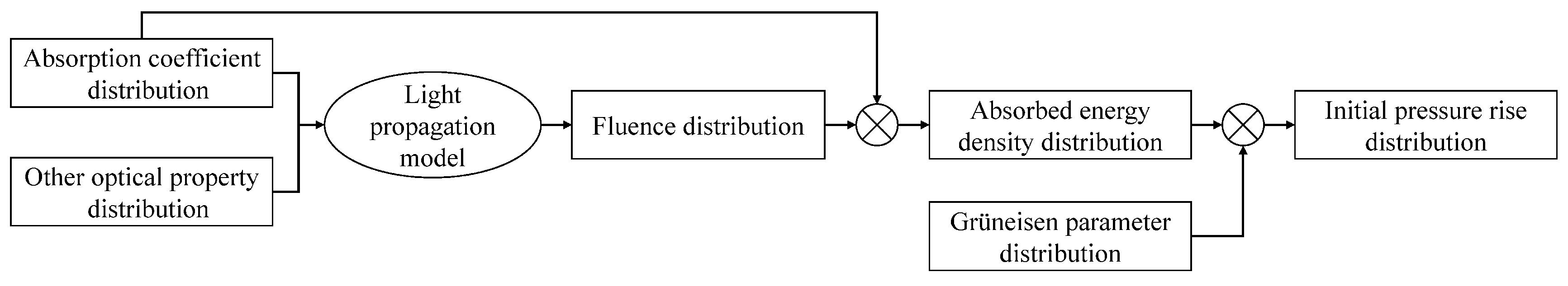
Table 1.
A brief summary of forward model-based methods.
| Category | Number of Forward Modeling | Advantages | Major Limitations |
|---|---|---|---|
| Fluence correction methods [9,41,42,43,44,45,46,47,48,49,50,51] | Single | Easy implementation; little computational load. | Extremely high dependence on predefined tissue properties, both geometrical and optical. |
| Model fitting methods [23,52,53] | Multiple | Certain applicability to unknown simple media; good computational efficiency. | Low accuracy due to the unrealistic optical homogeneity assumption. |
| Fixed-point iteration methods [54,55,56,57,58] | Iterative | High accuracy; high capability for unknown absorption distributions. | Requiring specified scattering distributions. |
| Minimization-based methods [59] | Iterative | Highest accuracy; high capability for all unknown optical property distributions. | Computationally intensive and time- consuming. |
Table 2.
A brief summary of all reviewed categories of methods.
| Category | Key Processes | Advantages | Limitations |
|---|---|---|---|
| Forward modeling-based methods | Utilizing a forward model to generate simulated counterparts of related variables. | Abundant choices of available frameworks with distinct features; a logically simple understanding due to the high conformity to the underlying physical process. | High dependence on the performance of the used light propagation model; a strict requirement of adequate knowledge of the experimental configurations. |
| Fluence correction via other techniques | Resorting to other techniques to measure the fluence map and correcting its impact. | Avoiding inherent complexity and limitations in the PA field. | Inherent drawbacks from the used assisted techniques; incorporating additional devices and procedures; compromising the system’s compactness. |
| Deep learning methods | Training deep neural networks to produce desired distributions in an end-to-end manner. | Significantly less dependence on prior knowledge of the object tissue and related physics; high computational efficiency in the implementation phase. | The extensive demand for training data labeled with true values and the lack of reliable in vivo measurement techniques; low generality of trained networks to system configurations and target scenario. |
| Decomposition-based methods | Decomposing related variables into a linear combination of a set of prescribed basis functions. | Producing acceptable results at a relatively less computational cost. | Very limited applicable cases due to the use of strong assumptions and the incomplete collection of basis functions. |
Disclaimer/Publisher’s Note: The statements, opinions and data contained in all publications are solely those of the individual author(s) and contributor(s) and not of MDPI and/or the editor(s). MDPI and/or the editor(s) disclaim responsibility for any injury to people or property resulting from any ideas, methods, instructions or products referred to in the content. |
© 2023 by the authors. Licensee MDPI, Basel, Switzerland. This article is an open access article distributed under the terms and conditions of the Creative Commons Attribution (CC BY) license (https://creativecommons.org/licenses/by/4.0/).
Share and Cite
MDPI and ACS Style
Wang, Z.; Tao, W.; Zhao, H. The Optical Inverse Problem in Quantitative Photoacoustic Tomography: A Review. Photonics 2023, 10, 487. https://doi.org/10.3390/photonics10050487
AMA Style
Wang Z, Tao W, Zhao H. The Optical Inverse Problem in Quantitative Photoacoustic Tomography: A Review. Photonics. 2023; 10(5):487. https://doi.org/10.3390/photonics10050487
Chicago/Turabian StyleWang, Zeqi, Wei Tao, and Hui Zhao. 2023. "The Optical Inverse Problem in Quantitative Photoacoustic Tomography: A Review" Photonics 10, no. 5: 487. https://doi.org/10.3390/photonics10050487
Note that from the first issue of 2016, this journal uses article numbers instead of page numbers. See further details here.