Determining Vortex-Beam Superpositions by Shear Interferometry


1
Department of Physics and Astronomy, Colgate University, Hamilton, NY 13346, USA
2
Departamento de Ciencias, Sección Física, Pontificia Universidad Católica del Peru, Apartado 1761, Lima, Peru
*
Author to whom correspondence should be addressed.
Photonics 2018, 5(3), 16; https://doi.org/10.3390/photonics5030016
Submission received: 17 May 2018
/
Revised: 19 June 2018
/
Accepted: 11 July 2018
/
Published: 14 July 2018
(This article belongs to the Special Issue Optical Angular Momentum in Nanophotonics)
Abstract
:Optical modes bearing optical vortices are important light systems in which to encode information. Optical vortices are robust features of optical beams that do not dissipate upon propagation. Thus, decoding the modal content of a beam is a vital component of the process. In this work, we present a method to decode modal superpositions of light beams that contain optical vortices. We do so using shear interferometry, which presents a simple and effective means of determining the vortex content of a beam, and extract the parameters of the component vortex modes that constitute them. We find that optical modes in a beam are easily determined. Its modal content can be extracted when they are of comparable magnitude. The use of modes of well-defined topological charge, but not well-defined radial-mode content, such as those produced by phase-only encoding, are much easier to diagnose than pure Laguerre–Gauss modes.
1. Introduction
Optical vortices are singular points contained in the transverse mode of beams of light. Around them, the phase of the light waves advances by an integer multiple of . They have attracted much attention in the last 25 years especially due to the intrinsic orbital angular momentum that they carry in the field surrounding the optical vortex [1]. Many applications of optical vortices have been found [2], and among them is the encoding of information for communication purposes, both classical [3,4] and quantal [5,6]. Spatial modes have become attractive for bearing information because optical vortices are particularly robust and recognizable features of beams. Although challenges remain in preserving the fidelity of spatial modes as the light propagates through media and turbulence [7], much promise remains [8,9,10,11]. The promise of this approach is the enhanced space of information bits, well beyond binary, and in principle unbound. Encoding can be done by use of vortices as an incoherent alphabet for communicating information [12] or as coherent superpositions of modes in a deliberate way [13] as a high-dimensional basis of states [14].
These developments have led to a number of methods to encode and decode optical-vortex structures in beams. In this work, we devote our attention to the detection of the vortex content of beams, and in particular superpositions. Numerous methods have been developed for the detection of optical modes of a beam bearing an optical vortex. They include non-collinear interferometry of the beam with itself [15], or in nested interferometers bearing parity-changing optical elements [16], or more simply, with single optical elements, such as a double slit [17], a single slit [18], a triangular aperture [19], cylindrical lenses [20], conformational optics [21], decoding by phase reconstruction and imaging [3,22], a shear interferometer [23] or a space-variant half-wave plate [24]. Beyond a beam carrying a singly- or multiply-charged vortex, it is quite necessary to be able to detect superpositions or to be able to sort the modal content of beams. Promising approaches include the use of projecting modes into the fundamental Gaussian mode [5,25], by unwrapping modes via conformational optics to spatially separate them [21,26] or by modal decomposition [22]. A more conventional approach is one that uses shear interferometry to recognize the vortex [27]. We also use shear interference by a single element, an extension of a method developed by two of us [23]. Some of the advantages of this method include: the use of very few optical elements, the determination of both the sign and magnitude of the vortices and its availability either commercially as a unit or easily constructed with standard optical components.
In this article, we present further use of the method by using it to determine the superposition of two beams each carrying an optical vortex. In such a situation, the vortices of the component beams are redistributed in a known way [28]. We use shear interferometry to unravel the pattern of vortices and determine the topological charge of each of the component beams. Furthermore, we discuss additional parameters of the superposition that can be obtained by this method: relative amplitude (within a range) and relative phase.
We start the article with the theoretical underpinnings, which are a summary of previous analyses adapted to the present problem [23,28]. This is divided into the two key aspects of the generated patterns: Section 2.1 for modal superpositions and Section 2.2 for shear interferometry. This is followed by the results divided into three sections: Section 3.1 for general features of the analysis with different types of beams: hypergeometric-Gauss, Laguerre–Gauss and Gaussian with phase encoding; Section 3.2 for the analysis of modal superpositions; and Section 3.3 for the determination of the relative weights of the component beams. A discussion of the results follows in Section 4. In the section on methods, we discuss: in Section 5.1, the details of the shear interferometer and the optical setup used, and in Section 5.2, an analysis of the shear patterns that determines the relative phase of each point in the image. Conclusions follow.
2. Theory
2.1. Modal Superpositions
Collinear superpositions of paraxial beams bearing optical vortices produce a composite mode where the location of the vortices reveals in a straightforward way the parameters of the superposition: the relative amplitude and phase of the component modes and their respective topological charge [28]. This is due to a basic feature of vortex beams: the modal pattern consists of a brightest inner ring with a radius that depends on the topological charge ℓ:
where a is a positive number. For pure Laguerre–Gauss beams, , where w is the beam half width.
Let us assume that the superposition of two vortex modes is given by:
where are the polar coordinates in the reference frame of the transverse mode, and are the topological charges of the two modes, specifies the ratio of the amplitudes of the two modes and is their relative phase. The functional expression for the modes is given by . We can distinguish two cases:
- When , the modal pattern is quite predictable and shows the following features:
- -
- The center of the pattern has an optical vortex of charge . This is what is theoretically predicted. In practice, a multiply-charged point is very susceptible to perturbations, and so, the center of the pattern may consist of singly-charged vortices of sign in close proximity.
- -
- The center is surrounded by vortices arranged symmetrically [28] and located at a radial distance that satisfies:For the case of pure Laguerre–Gauss modes, we know the analytical expressions of , and so, we can deduce :The angular position of the vortices depends on the relative phase between the two modes [28]:where is an odd integer.
For example, when and , the composite mode for consists of a central vortex of charge surrounded by three vortices of charge located at a radius . - When and , the pattern contains a central vortex of charge . At , there is no central vortex, and the composite mode has radial lines (nodes) of shear phase, evenly separated. The relative weights of the modes produce subtle variations in intensity, which yields greater uncertainty in the determination. The method presented in this article is much more effective for the first case.
2.2. Shear Interference Pattern
The shear interference pattern of a beam bearing an optical vortex of topological charge ℓ has the following characteristics [23] (details of the interferometer and a visual schematic of the angular parameters are shown in Section 5.1):
- The pattern consists of conjoined forks formed by the interference of the vortex beam with a displaced and tilted copy of it. If the shear interferometer is air spaced, the centers of the vortices are displaced by:where is the incident angle and t is the average separation between the reflecting surfaces. This relation is modified if the fringes are not parallel to the displacement of the two modes.
- The overall phase of the pattern is determined by the optical path-length difference and the reflection phases, which for our case is given by:where is the wavelength of the light.
- The fringe density of the pattern is given by:where:is the angle that the back reflection makes with the horizontal. We use the convention when the beam coming from the back reflection is tilted downward and assuming that the front reflection is in the horizontal plane. is the wedge angle between the two reflecting surfaces.
When the interferometer is a solid piece, which we have used in the past [23,29], these relations are modified slightly [30]. We found the air-spaced interferometer very convenient for freely changing the above parameters. In a typical situation, aiming for a total of 15 fringes over the full size of the beam of 4 mm (with ) requires a tilt arcmin. The pattern representing an optical vortex consists of forks joined by their handles or their tines when the topological charge is positive or negative, respectively, as discussed below. The correlation between the patterns and sign of the topological charge switches when .
3. Results
3.1. Mode Comparison
The effectiveness of the method depends on the radial dependence of the vortex mode. The best modes are those where the dark regions around the vortices are small relative to the beam diameter. This is because the pattern is the interference of two displaced identical modes. Such modes are the ones generated, for example, with a forked diffraction grating [31], spiral phase plate [32] or digital phase modulation [33,34]; and known as hypergeometric-Gaussian modes [35] or Kummer modes, which are expressed in terms of Bessel functions [36,37,38]. Laguerre–Gauss modes are categorized by two indices: the azimuthal index or topological charge ℓ and the radial index p specifying the number of nodes in the radial coordinate. Pure modes are the hardest to diagnose. This is because most of the light intensity is limited to a well-defined ring, and so, the signal to noise ratio of the interference patterns is low in the dark regions. Hypergeometric-Gaussian modes generated by phase-only encoding are in a superposition of Laguerre–Gauss modes of the same ℓ, but different p [15,39]. Such modes modes have intensity patterns featuring a main ring surrounded by broad radial modulations. They are much better because most regions of overlap of the modes have non-zero intensity and thus produce good fringe visibilities. When investigations are limited to a laboratory area, it is often convenient to image the mode encoding element via a four-f sequence of lenses. That way, the beam reconstructed on the camera is nearly a Gaussian (the input to the encoding device), with the phase encoding. Imperfections in the encoding, imaging apparatus and diffraction itself make the modes with distinct topological charge distinct, as well, enabling optical processing with such modes. We call this type of imaging “near field.”
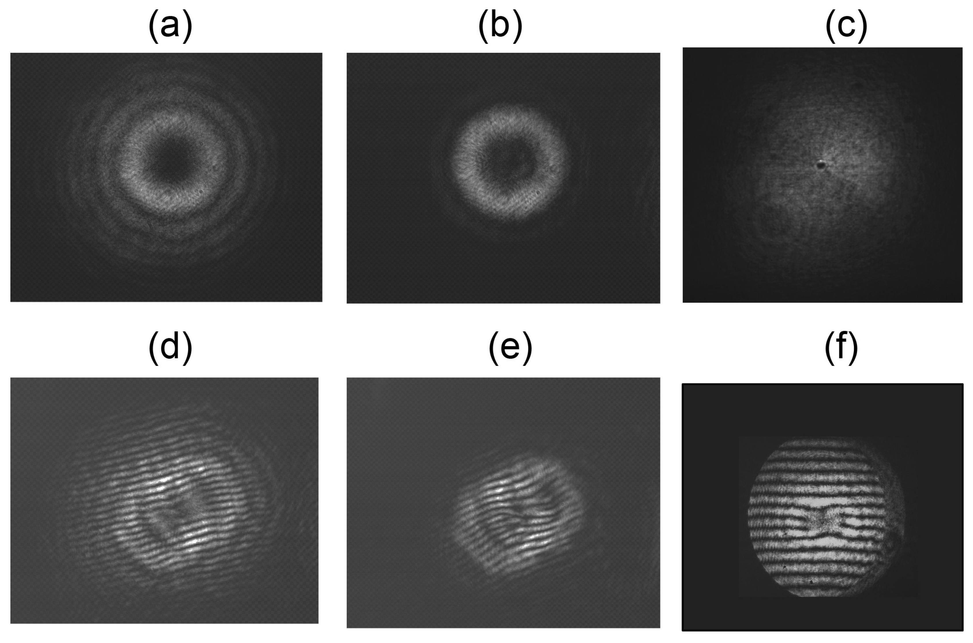
Figure 1 shows three types of modes that we prepared with a spatial light modulator and their corresponding shear interference pattern below. They were taken with our air-spaced interferometer, which allowed us to adjust the plate separation. The modes were generated by diffraction off the phase grating of a spatial light modulator with and without amplitude modulation. The amplitude modulation produced a pure Laguerre–Gauss mode (Figure 1b), while the lack of amplitude modulation produced a hypergeometric-Gauss mode (Figure 1a) as described above. Near-field imaging produced a Gaussian mode with phase encoding (Figure 1c). Pure Laguerre–Gauss modes are much harder to determine because they contain more than one ring, with consecutive rings being out of phase. This feature complicates the pattern produced by the shear interferometer. The darkened regions in the modes of Figure 1a–c are candidates for locations bearing optical vortices, but only the shear interference pattern can confirm the association of darkened regions with vortices.
3.2. Determining the Topological Charge of the Component Beams
The main virtue of the method presented in this article involves identifying superpositions of vortex-modes. When this involves equal-amplitude superpositions ( in Equation (2)), we can clearly determine the modes, regardless of type. Beyond inspecting the static images of the patterns, we can determine the relative phase of each image point by slightly varying the incident angle of the light on the shear interferometer and fitting the phase of the pattern, as described in Section 5.2. We show such a sequence in Movie 1.
Figure 2 shows the example of the superposition of with (). We use the Gaussian mode with phase encoding to best appreciate the method. The modes are determined using the following procedure:
- We first examine the fork pattern in the center of the mode. From it, we extract the magnitude and sign of the mode with smaller topological charge (recall that we assume ). No vortices means . In the case of Figure 2b, we see the conjoined-fork pattern of a vortex, revealing that . In the table in Figure 2a, we give the correspondence between the sign of the topological charge of the vortex and its forked signature in the shear pattern.
- We count the number of peripheral vortices N (in Figure 2b, we see that ). The type of conjoined forks specifies their sign. If the sign of peripheral vortices is the same as the one at the center, then:If the sign is different than the center vortex, then:In our example of Figure 2b, because the sign of the peripheral vortices is different from the one of the central vortex, we conclude that .
- The angular orientation of the vortices reveals the relative phase between the modes per Equation (5). In our example, .
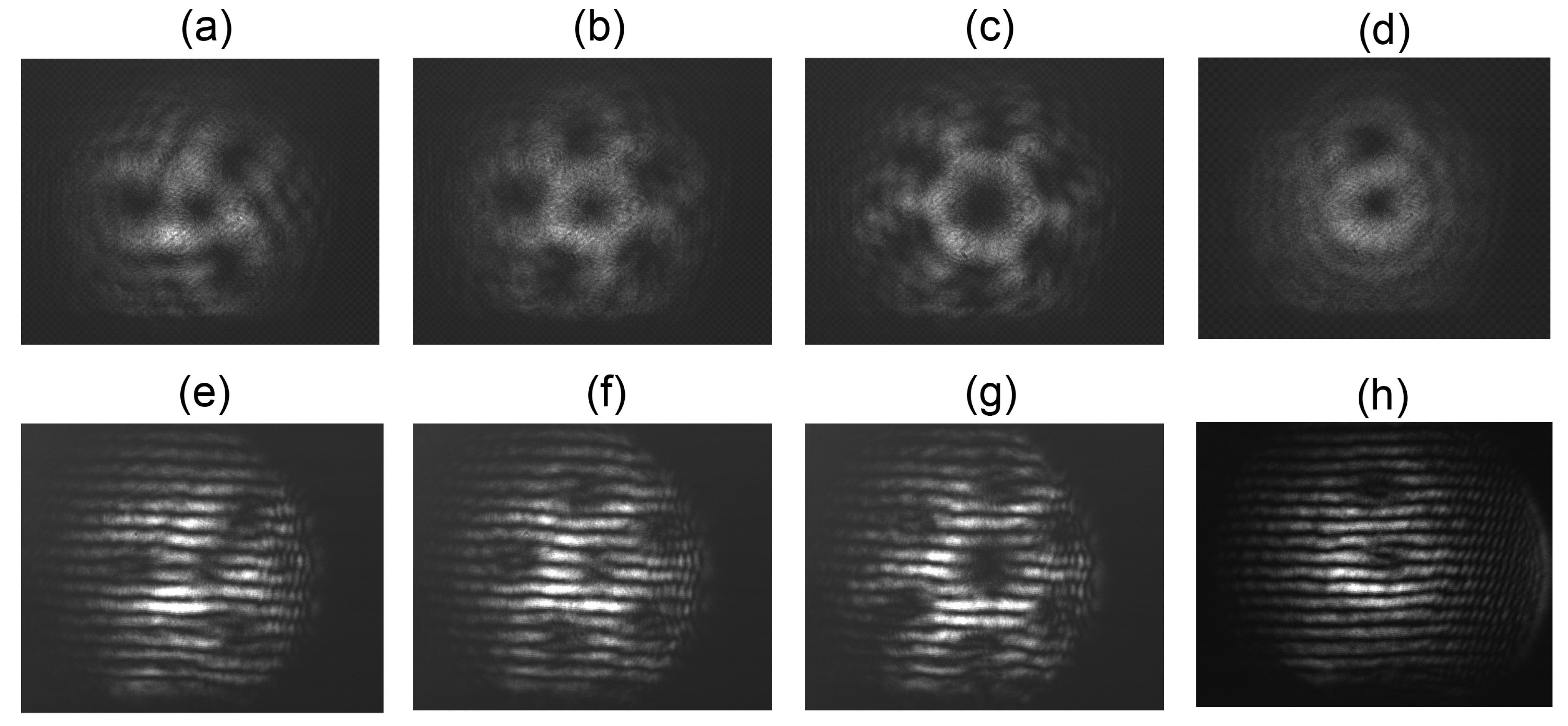
Figure 3 shows four cases with distinct values of : , , and . The figure shows views of the mode images in Panes (a–d) and the shear interferograms in (e–h). All cases were taken in the far field produced by the non-amplitude modulated encoding. The mode images show dark regions where the vortices are located. The presence of a vortex is only confirmed by the appearance of the forked dislocations in the interferograms. The first case (a,e) is similar to the one in Figure 2b, featuring one central +1 vortex surrounded by three vortices. The second case in (b,f) has again a central vortex surrounded by five vortices. The third case with underscores the method, showing a central vortex, surrounded by six vortices. The case involves . When , the peripheral vortex is along the horizontal axis of the pattern. When the fringes are lined up along the direction connecting the centers of the displaced modes, two forks connected by their handle reveal positive vortices, whereas two forks conjoined by the tines reveal negative vortices. If the alignment is not as good, then the conjoined forks are laterally displaced, as illustrated in Figure 2a, so that for example, in the case of negative vortices, the forks share only one tine. They can also share no tines and just be laterally displaced. We can also make adjustments to a second tilt of the air-spaced interferometer to tilt the fringes along the direction that connects the centers of the displaced vortices. The case of Figure 2b shows clearly that the forks representing each vortex are joined by both tines. Depending on the value of the local phase difference between the two interfering reflections, the forks are more clearly observed either via the bright or dark fringes.
3.3. Determining the Relative Amplitude of the Component Beams
The comparisons of the previous cases involve equal-amplitude superpositions. For a certain range of parameters, we can determine the superposition of modes with unequal amplitudes. A superposition can be determined as long as light from one reflection overlaps with all vortex locations of the other reflection, and vice versa. Such a situation is the requirement for producing a measurable fork pattern for each vortex. In the case of the pure Laguerre–Gauss modes, the settings of the shear interferometer (separation and tilt) have to be adjusted for the particular situation, whereas for the hypergeometric-Gauss or Gaussian with phase encoding, no specific settings are required.
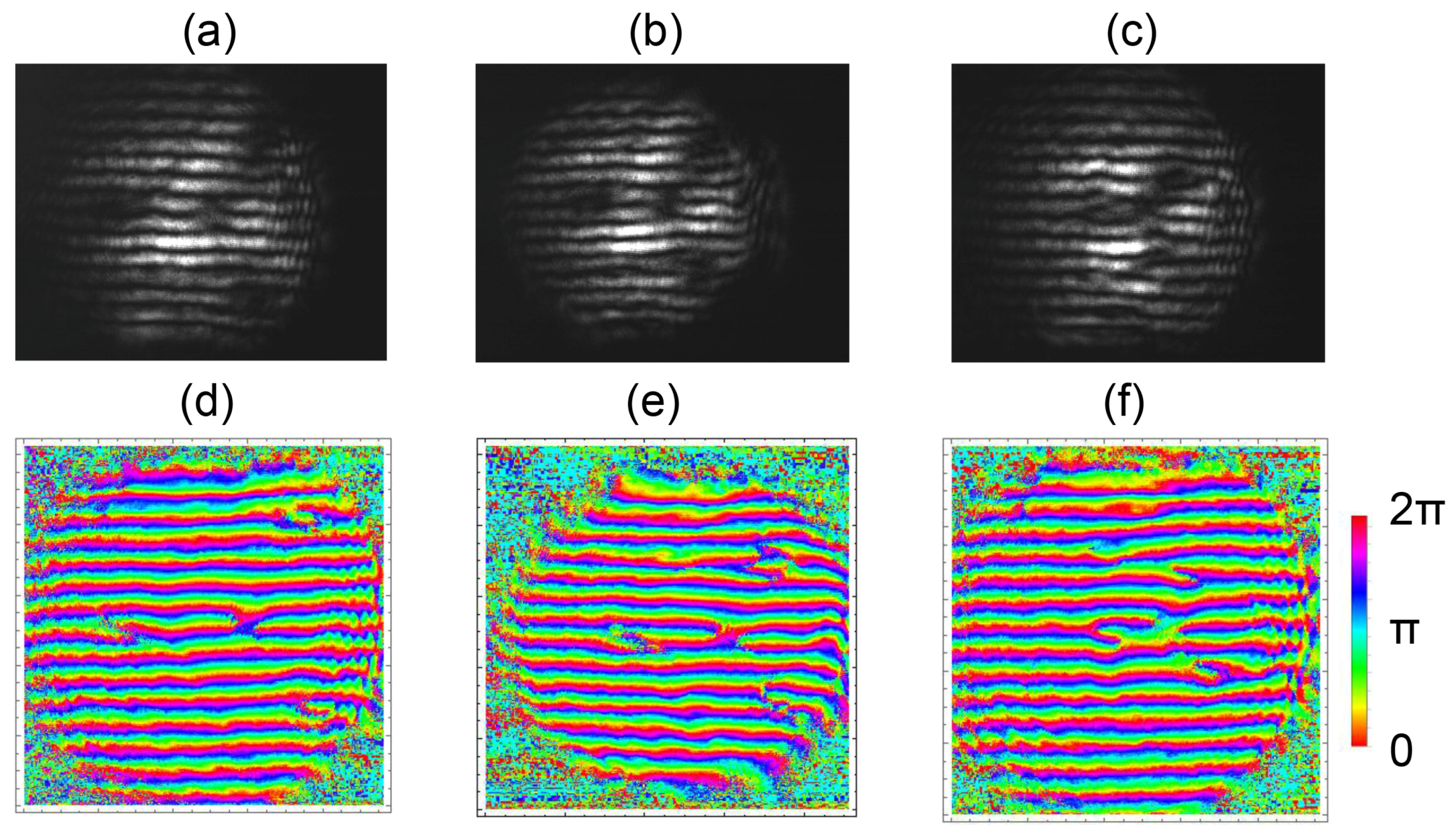
The peripheral vortices that surround the central vortex, located at a radius , are seen as long as , where R is the visible radius of the beam. This sets a lower bound for the value of in Equation (2), which depends on the type of vortex mode: lower for non-Laguerre–Gauss modes. The pattern of the case of in Figure 4a was created with . The peripheral vortices are close to the edge of the beam. Depending on the type of mode, can be between and .
In a similar manner, as , the singly-charged vortices reach the center to form a region of charge . For , it is not possible to distinguish clearly the central vortex from the peripheral vortices, and so, we cannot identify the component modes. From our own experience, . Figure 4c shows the case for . We have taken sequences of a number of cases with varying values of , and . In Movie 2, we show the case for a sequence of values.
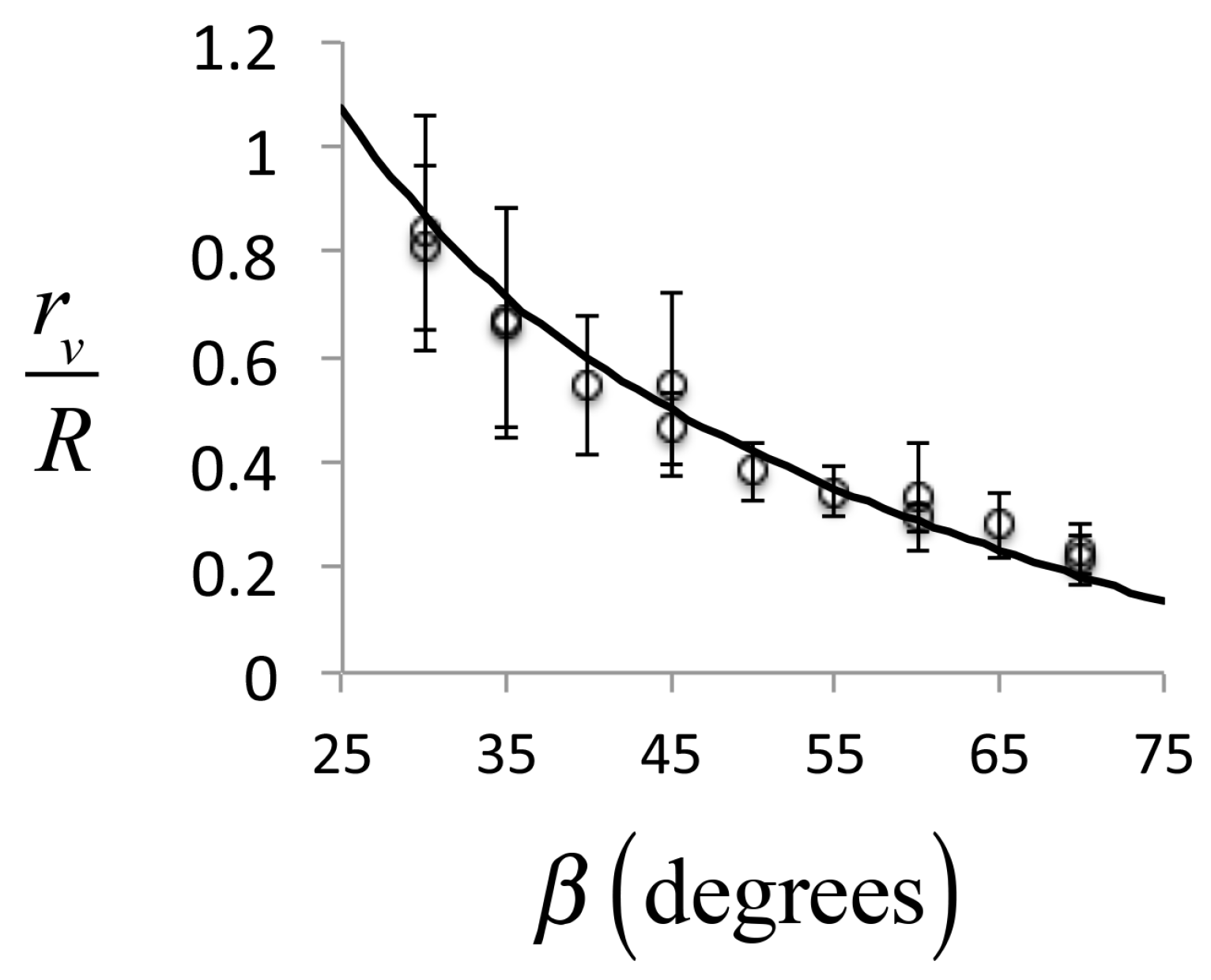
We did an analysis of the variation of with by measuring the values of in the images. In Figure 5, we show as a function of for the case of . The uncertainties are standard deviations of the measurements. We compare those measurements with the predicted value of scaled by a factor of . We found similar agreement with two other cases that we studied, but using other scalings.
4. Discussion
The analysis shown above shows that shear interferometry can be used to identify the topological charges of modes in superpositions. We can do this determination for most pure or semi-pure modes bearing optical vortices. We have shown this with modes imaged in the far field, as well as in the near field [29]. The method can be used to determine the relative weights of the two modes when their amplitudes are not too dissimilar (in the language of Equation (2), for ). The results of this article apply for modes in the far field, which may be used in communications. If the use of vortex beams is limited to the laboratory environment, one can use engineered near-field patterns, which allow greater flexibility in the encoding of vortices [13] and greater ease in their detection by shear interferometry [29].
The identification of modal superpositions presented here was done with an air-spaced shear interferometer that we built. This gives much flexibility in the adjustment of the interferometer angles for setting a pattern that best suits the modal determinations. These determinations can also be done with a commercially available single-plate shear interferometer, as reported recently [23,29].
5. Apparatus and Methods
5.1. Shear Interferometer
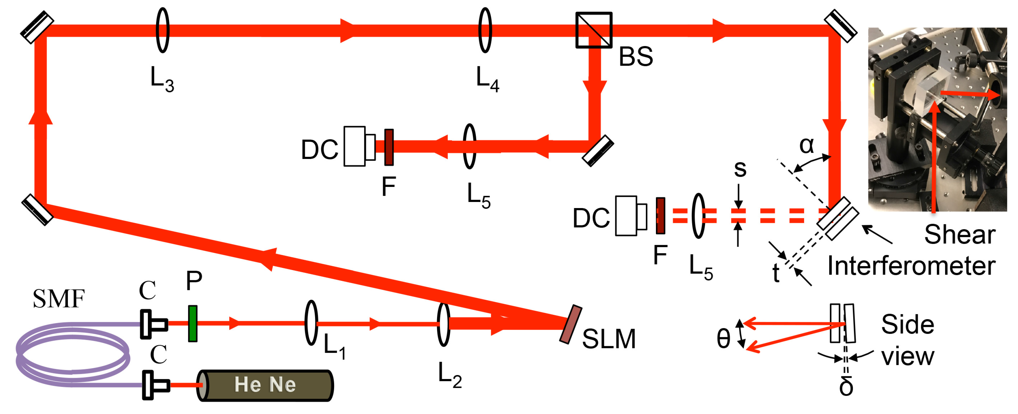
In this work, we used an air-spaced shear interferometer shown in the insert to Figure 6. It consisted of two thick (∼5 mm) uncoated wedged glass blanks mounted in such a way that the one responsible for the back reflection was mounded in a mirror-type mount, so that its tilt could be adjusted. The blank responsible for the first reflection, made of Vycor glass (), was mounted on a translating mount to enable adjustment of the separation t between the two surfaces causing the interference pattern. The entire interferometer was mounted on a rotation stage that allowed slight variations in the incident angle . We used the latter to change the phase between the two reflections. The data were taken for , which corresponds to an internal angle of incidence on the shear gap of .
The entire layout of our optical setup is shown in Figure 6. The output of a helium-neon laser was spatially filtered by passage through a single-mode fiber (SMF) coupled to collimators (C). The polarization of the beam was adjusted for optimal diffraction with a spatial light modulator (SLM). The light incident on it was expanded via lenses L and L. The first-order diffraction off the SLM was expanded further with lenses L and L and divided by a beam splitter to observe the mode with the digital camera. The second beam expansion was needed for a greater overlap of the two sheared reflections. The light transmitted by the beam splitter was steered onto the shear interferometer. We also used a single-element shear interferometer to insure that the input beam had a maximum radius of curvature. The beam bearing the shear interference pattern was slightly focused by a lens to fit the mode within the digital camera sensing element.
5.2. Shear-Pattern Analysis
The shear interferometer has the flexibility to allow the change in the phase of the interference pattern by slightly varying the incident angle : a 3-arcmin change per fringe shift using Equation (7). As mentioned above, we collected a movie of the pattern for at least one fringe shift. We used these data to fit the period of the pattern in a sequence of images. The outcome of that fit was used as a fixed parameter to fit the phase of each imaged point. The outcome of this analysis yielded the phase patterns of the type shown in Figure 2 and Figure 4. The phase of the pattern allows a straightforward determination of the vortices, and from them, we can find the topological charge of the component beams. We used this procedure as an alternative to the determination of vortices directly from the interferograms. This procedure can be automated further using an algorithm to make an automatic determination of the location of the vortices and their topological charge.
6. Conclusions
We presented a robust method to determine the topological charges of modal superpositions based on shear interferometry. The method relies on the interference of an incoming beam with itself, so it does not rely on a reference beam. The key aspect of the method is that it is simple and robust. Optical vortices are arranged in a predictable way that can be used to make the modal determinations. This includes a range of the relative weights of the two vortex modes in the superposition and their relative phase. The method presented here can be used to identify vortex modes when they are inserted in optical beams for the purpose of encoding information. This method may also be used as a diagnosis tool when using optical vortices in biomedical applications or nanotechnology.
Author Contributions
Conceptualization and Methodology, B.K. and E.J.G.; Data Acquisition, B.K. and J.R.G.U.; Analysis, B.K., J.R.G.U. and E.J.G.; Writing, E.J.G.
Funding
This research was funded by the National Science Foundation Grant Number PHY1506321.
Conflicts of Interest
The authors declare no conflict of interest. The founding sponsors had no role in the design of the study; in the collection, analyses or interpretation of data; in the writing of the manuscript; nor in the decision to publish the results.
References
- Allen, L.; Beijersbergen, M.; Spreeuw, R.; Woerdman, J. Orbital angular momentum of light and the transformation of Laguerre–Gaussian laser modes. Phys. Rev. A 1992, 45, 8185–8189. [Google Scholar] [CrossRef] [PubMed]
- Rubinsztein-Dunlop, H.; Forbes, A.; Berry, M.V.; Dennis, M.R.; Andrews, D.L.; Mansuripur, M.; Denz, C.; Alpmann, C.; Banzer, P.; Bauer, T.; et al. Roadmap on structured light. J. Opt. 2017, 19, 013001. [Google Scholar] [CrossRef]
- Gibson, G.; Courtial, J.; Padgett, M.; Vasnetsov, M.; Pas’ko, V.P.; Barnett, S.; Franke-Arnold, S. Free-space information transfer using light beams carrying orbital angular momentum. Opt. Express 2004, 12, 5448–5456. [Google Scholar] [CrossRef] [PubMed]
- Wang, J.; Yang, J.Y.; Fazal, I.M.; Ahmed, N.; Yan, Y.; Huang, H.; Ren, Y.; Yue, Y.; Dolinar, S.; Tur, M.; et al. Terabit free-space data transmission employing orbital angular momentum multiplexing. Nat. Photonics 2012, 340, 488–496. [Google Scholar] [CrossRef]
- Mair, A.; Vaziri, A.; Weihs, G.; Zeilinger, A. Entanglement of the orbital angular momentum states of photons. Nature 2001, 412, 313–316. [Google Scholar] [CrossRef] [PubMed] [Green Version]
- Molina-Terriza, G.; Torres, J.; Torner, L. Twisted photons. Nat. Phys. 2008, 3, 305–310. [Google Scholar] [CrossRef]
- Rodenburg, B.; Lavery, M.; Malik, M.; O’Sullivan, M.; Mirhosseini, M.; Robertson, D.; Padgett, M.; Boyd, R. Influence of atmospheric turbulence on states of light carrying orbital angular momentum. Opt. Lett. 2012, 37, 3735–3737. [Google Scholar] [CrossRef] [PubMed]
- Malik, M.; O’Sullivan, M.; Rodenburg, B.; Mirhosseini, M.; Leach, J.; Lavery, M.P.J.; Padgett, M.; Boyd, R. Influence of atmospheric turbulence on optical communications using orbital angular momentum for encoding. Opt. Express 2012, 20, 13195–13200. [Google Scholar] [CrossRef] [PubMed] [Green Version]
- D’Ambrosio, V.; Nagali, E.; Walborn, S.; Aolita, A.; Slussarenko, S.; Marrucci, L.; Sciarrino, F. Complete experimental toolbox for alignment-free quantum communication. Nat. Commun. 2012, 3, 961. [Google Scholar] [CrossRef] [PubMed] [Green Version]
- Ren, Y.; Wang, Z.; Xie, G.; Li, L.; Willner, A.; Cao, Y.; Zhao, Z.; Yan, Y.; Ahmed, N.; Ashrafi, N.; et al. Atmospheric turbulence mitigation in an OAM-based MIMO free-space optical link using spatial diversity combined with MIMO equalization. Opt. Lett. 2016, 41, 2406–2409. [Google Scholar] [CrossRef] [PubMed]
- Krenn, M.; Handsteiner, J.; Fink, M.; Fickler, R.; Ursin, R.; Malik, M.; Zeilinger, A. Twisted light transmission over 143 km. Proc. Natl. Acad. Sci. USA 2016, 113, 13648–13653. [Google Scholar] [CrossRef] [PubMed]
- Krenn, M.; Fickler, R.; Fink, M.; Handsteiner, J.; Malik, M.; Scheidl, T.; Ursin, R.; Zeilinger, A. Communication with spatially modulated light through turbulent air across Vienna. New J. Phys. 2014, 16, 113028. [Google Scholar] [CrossRef] [Green Version]
- Molina-Terriza, G.; Torres, J.; Torner, L. Management of the angular momentum of light: Preparation of photons in multidimensional vector states of angular momentum. Phys. Rev. Lett. 2002, 88, 013601. [Google Scholar] [CrossRef] [PubMed]
- Barreiro, J.; Langford, N.; Peters, N.; Kwiat, P. Generation of hyperentangled photon pairs. Phys. Rev. Lett. 2005, 95, 260501. [Google Scholar] [CrossRef] [PubMed]
- Heckenberg, N.; McDuff, R.; Smith, C.; Rubinsztein-Dunlop, H.; Wegener, M. Laser beams with phase singularities. Opt. Quanum Electron. 1992, 24, 355–361. [Google Scholar] [CrossRef]
- Leach, J.; Padgett, M.J.; Barnett, S.M.; Franke-Arnold, S.; Courtial, J. Measuring the orbital angular momentum of a single photon. Phys. Rev. Lett. 2002, 88, 257901. [Google Scholar] [CrossRef] [PubMed]
- Sztul, H.I.; Alfano, R.R. Double-slit interference with Laguerre–Gaussian beams. Opt. Lett. 2006, 31, 999–1001. [Google Scholar] [CrossRef] [PubMed]
- Ferreira, Q.; Jesus-Silva, A.; Fonseca, E.; Hickmann, J. Fraunhofer diffraction of light with orbital angular momentum by a slit. Opt. Lett. 2011, 36, 3106–3108. [Google Scholar] [CrossRef] [PubMed]
- Hickmann, J.; Fonseca, E.; Soares, W.; Chavez-Cerda, S. Unveiling a truncated optical lattice associated with a triangular aperture using light’s orbital angular momentum. Phys. Rev. Lett. 2010, 105, 053904. [Google Scholar] [CrossRef] [PubMed]
- Beijersbergen, M.W.; Allen, L.; van der Veen, H.E.L.O.; Woerdman, J.P. Astigmatic laser mode converters and transfer of orbital angular momentum. Opt. Commun. 1993, 96, 123–132. [Google Scholar] [CrossRef]
- Berkhout, G.C.; Lavery, M.P.; Courtial, J.; Beijersbergen, M.W.; Padgett, M.J. Efficient sorting of orbital angular momentum states of light. Phys. Rev. Lett. 2010, 105, 153601. [Google Scholar] [CrossRef] [PubMed]
- Schulze, C.; Dudley, A.; Flamm, D.; Duparré, M.; Forbes, A. Measurement of the orbital angular momentum density of light by modal decomposition. New J. Phys. 2013, 15, 073025. [Google Scholar] [CrossRef] [Green Version]
- Khajavi, B.; Galvez, E. Determining topological charge of an optical beam using a wedged optical flat. Opt. Lett. 2017, 42, 1516–1519. [Google Scholar] [CrossRef] [PubMed]
- Liu, G.G.; Wang, K.; Lee, Y.H.; Wang, D.; Li, P.P.; Gou, F.; Li, Y.; Tu, C.; Wu, S.T.; Wang, H.T. Measurement of the topological charge of vortex vector optical fields with a space-variant half-wave plate. Opt. Lett. 2018, 43, 823–826. [Google Scholar] [CrossRef] [PubMed]
- Jack, B.; Leach, J.; Ritsch, H.; Barnett, S.; Padgett, M.; Franke-Arnold, S. Precise quantum tomography of photon pairs with entangled orbital angular momentum. New J. Phys. 2009, 11, 103024. [Google Scholar] [CrossRef] [Green Version]
- O’Sullivan, M.; Mirhosseini, M.; Malik, M.; Boyd, R. Near-perfect sorting of orbital angular momentum and angular position states of light. Opt. Express 2012, 20, 24444. [Google Scholar] [CrossRef] [PubMed]
- Ghai, D.P.; Senthilkumaran, P.; Sirohi, R. Shearograms of an optical phase singularity. Opt. Commun. 2008, 281, 1315–1322. [Google Scholar] [CrossRef]
- Baumann, S.; Kalb, D.; MacMillan, L.; Galvez, E. Propagation dynamics of optical vortices due to Gouy phase. Opt. Express 2009, 17, 9818–9827. [Google Scholar] [CrossRef] [PubMed]
- Khajavi, B.; Galvez, E. Determination of the topological charge of complex light beams by shearing interference from a wedged optical flat. Proc. SPIE 2018, 10549, 105490M. [Google Scholar]
- Riley, M.E.; Gusinow, M.A. Laser beam divergence utilizing a lateral shearing interferometer. Appl. Opt. 1977, 16, 2753–2756. [Google Scholar] [CrossRef] [PubMed]
- Bazhenov, V.; Vatnetsov, M.; Soskin, M. Laser beams with screw dislocations in their wavefronts. JETP Lett. 1990, 52, 1037–1039. [Google Scholar]
- Beijersbergen, M.; Coerwinkel, R.; Kristensen, M.; Woerdman, J. Helical-wavefront laser beams produced with a spiral phaseplate. Opt. Commun. 1994, 112, 321–327. [Google Scholar] [CrossRef]
- Curtis, J.; Grier, D. Structure of optical vortices. Phys. Rev. Lett. 2003, 90, 133901. [Google Scholar] [CrossRef] [PubMed]
- Leach, J.; Yao, E.; Padgett, M. Observation of the vortex structure of a non-integer vortex beam. New J. Phys. 2004, 6, 71. [Google Scholar] [CrossRef]
- Karimi, E.; Zito, G.; Piccirillo, B.; Marrucci, L.; Santamato, E. Hypergeometric-Gaussian modes. Opt. Lett. 2007, 32, 3053–3055. [Google Scholar] [CrossRef] [PubMed]
- Berry, M. Optical vortices evolving from helicoidal integer and fractional phase steps. J. Opt. A Pure Appl. Opt. 2004, 6, 259–268. [Google Scholar] [CrossRef]
- Basistiy, I.; Pas’ko, V.; Slyusar, V.; Soskin, M.; Vasnetsov, M. Synthesis and analysis of optical vortices with fractional topological charges. J. Opt. A Pure Appl. Opt. 2004, 6, S166–S169. [Google Scholar] [CrossRef]
- Bekshaev, A.; Karamoch, A. Spatial characteristics of vortex light beams produced by diffraction gratings with embedded phase singularity. Opt. Commun. 2008, 281, 1366–1374. [Google Scholar] [CrossRef]
- Sephton, B.; Dudley, A.; Forbes, A. Revealing the radial modes in vortex beams. Appl. Opt. 2016, 55, 7830–7835. [Google Scholar] [CrossRef] [PubMed]
Figure 1.
Beam modes (a–c) and corresponding shear interferograms (d–f) of vortex beams generated using phase modulation only (a,c), phase and amplitude modulation (b) and far-field (a,b) and near-field imaging (c). All modes have .
Figure 1.
Beam modes (a–c) and corresponding shear interferograms (d–f) of vortex beams generated using phase modulation only (a,c), phase and amplitude modulation (b) and far-field (a,b) and near-field imaging (c). All modes have .

Figure 2.
(a) Table showing the conditions that lead to distinct shear patterns of optical vortices along with their signature in the pattern. corresponds to the second reflection deflected downward relative to the first reflection off the shear interferometer. (b) Phase pattern of the shear interference of the superposition of modes with topological charges and . We label the arrangement of vortices produced by the superposition. The measured radial distance of the vortices is taken as the distance between the center of the central pattern and the center of each of the peripheral vortices.

Figure 3.
Images of equal-amplitude superpositions of modes with topological charges in (a), in (b), in (c) and in (d). The images in the second row (e–h) are the shear interferograms of the superpositions above them.
Figure 3.
Images of equal-amplitude superpositions of modes with topological charges in (a), in (b), in (c) and in (d). The images in the second row (e–h) are the shear interferograms of the superpositions above them.

Figure 4.
Top row: shear interferograms of the superposition of modes with topological charges and for several values of : in (a), in (b) and in (c). Bottom row (d–f): reconstructions of the phase of the light field corresponding to the shear patterns above them. False color encodes phase.
Figure 4.
Top row: shear interferograms of the superposition of modes with topological charges and for several values of : in (a), in (b) and in (c). Bottom row (d–f): reconstructions of the phase of the light field corresponding to the shear patterns above them. False color encodes phase.

Figure 5.
Graph of the radial position of the peripheral vortices relative to the beam radius as a function of the parameter that determines the ratio of the amplitudes of the modes in Equation (2). The data shown correspond to the case . The solid line corresponds to the in Equation (4).

Figure 6.
Apparatus used to make the measurements. Components include the spatial light modulator (SLM) lenses (L), fiber collimators (C), single-mode fiber (SMF), beam splitter (BS), polarizer (P), neutral density filters (F) and digital camera (DC). The insert shows a photo of the shear interferometer. The diagram also shows the relevant parameters of the interferometer: the angle of incidence , the shear displacement s, the shear-plate separation t and second plate tilt .

© 2018 by the authors. Licensee MDPI, Basel, Switzerland. This article is an open access article distributed under the terms and conditions of the Creative Commons Attribution (CC BY) license (http://creativecommons.org/licenses/by/4.0/).
Share and Cite
MDPI and ACS Style
Khajavi, B.; Ureta, J.R.G.; Galvez, E.J. Determining Vortex-Beam Superpositions by Shear Interferometry. Photonics 2018, 5, 16. https://doi.org/10.3390/photonics5030016
AMA Style
Khajavi B, Ureta JRG, Galvez EJ. Determining Vortex-Beam Superpositions by Shear Interferometry. Photonics. 2018; 5(3):16. https://doi.org/10.3390/photonics5030016
Chicago/Turabian StyleKhajavi, Behzad, Junior R. Gonzales Ureta, and Enrique J. Galvez. 2018. "Determining Vortex-Beam Superpositions by Shear Interferometry" Photonics 5, no. 3: 16. https://doi.org/10.3390/photonics5030016
Note that from the first issue of 2016, this journal uses article numbers instead of page numbers. See further details here.