Overcoming Challenges in Large-Core SI-POF-Based System-Level Modeling and Simulation

Abstract

The application areas for plastic optical fibers such as in-building or aircraft networks usually have tight power budgets and require multiple passive components. In addition, advanced modulation formats are being considered for transmission over plastic optical fibers (POFs) to increase spectral efficiency. In this scenario, there is a clear need for a flexible and dynamic system-level simulation framework for POFs that includes models of light propagation in POFs and the components that are needed to evaluate the entire system performance. Until recently, commercial simulation software either was designed specifically for single-mode glass fibers or modeled individual guided modes in multimode fibers with considerable detail, which is not adequate for large-core POFs where there are millions of propagation modes, strong mode coupling and high variability. These are some of the many challenges involved in the modeling and simulation of POF-based systems. Here, we describe how we are addressing these challenges with models based on an intensity-vs-angle representation of the multimode signal rather than one that attempts to model all the modes in the fiber. Furthermore, we present model approaches for the individual components that comprise the POF-based system and how the models have been incorporated into system-level simulations, including the commercial software packages Simulink^TM and ModeSYS^TM.

1. Introduction

For many years now, researchers across the globe have been reporting experiments demonstrating the feasibility of transmitting high-speed data over different types of plastic optical fibers (POFs). Due to the high-loss of POF (~100–300 dB/km), its application was discussed in the context of short-reach in-home [1,2] and automotive networks [3]. More recently, POF has been suggested as a transmission medium for avionic platforms as well [4]. While the experimental results are quite impressive, the modeling and simulation of POF links have not kept pace; commercial software packages have only recently begun to add support for system-level modeling of POFs. POF-based communication systems are usually operated close to their capacity, which is limited by the scarce power budget, the reduced bandwidth or a combination of both. Moreover, the growing demand for higher data rates is challenging the capability of SI-POFs to supply enough bandwidth even in these restricted environments and is compelling researchers to investigate different technologies to enhance spectral efficiency [5,6,7,8,9]. Therefore, it is essential that the system performance using new transmission techniques be estimated and the design be optimized before the system is physically deployed. The tight power budget and multiple components comprising the POF-based system make the use of a rigorous, experimentally validated simulation framework, with proven predictive capabilities, a crucial tool in assessing the end-to-end system performance.

There are a few different types of POFs available in the market whose key distinguishing features lay in the properties of the material used for the core and cladding (related to the refractive index profile), the diameter of an individual core, the number of cores, and the refractive index profile. Each POF type possesses a set of unique characteristics that makes it particularly suitable for specific data network scenarios [10]. For short-range data transmission, the step-index plastic optical fiber (SI-POF) is a competitive media for low-cost applications. Although, recently, multicore step-index plastic optical fiber (MC SI-POF) and graded-index plastic optical fiber (GI-POF) have garnered attention due to their potentially greater bandwidths. Although poly-methyl methacrylate (PMMA)-based POF exhibits its best transmission performance when operating at the visible end of the spectrum, supporting red and green light sources, its attenuation is often higher than can be tolerated by some applications. Thus, researchers have been working on alternatives that inherently have lower loss and support transmission in the infrared region of the spectrum, where high-quality light sources are more readily available. Partially fluorinated methacrylate polymer such as poly (2,2,2-trifluoroethyl methacrylate) (P3FMA)-based GI-POF, with an attenuation coefficient of 71 dB/km, was shown to be superior to the PMMA-based POF, not only in terms of lower attenuation but also due to its lower modal dispersion [11]. Perfluorinated graded-index plastic optical fiber (PF GI-POF) with a core diameter of 50–120 µm is emerging with even better performance than the P3FMA. Losses of 50 dB/km and lower in the wavelength range 600–1300 nm are now being realized [12,13].

Over the years, different approaches to simulate optical power transmission in large-core POFs have been devised in an attempt to achieve a compromise between precision and computation time. Ray-tracing provides a highly intuitive approach that has been successfully applied to describe light propagation not only in SI-POFs [14], but also in MC-POFs and GI-POFs [15,16,17] and has also been adapted to research the effects of perturbations on light transmission [18]. While ray-tracing is flexible to incorporate constraints that describe different situations, its obvious drawback is the required computational time that prevents its use for system-level simulations. Particularly, and in contrast to glass optical fiber models, the strong diffusion of PMMA and the core-cladding surface roughness of POFs induce power transfer between neighboring mode groups or mode coupling, that can be modeled following different approaches. In the case of ray-tracing, this effect is described by a random change of the propagation direction that occurs after propagation up to a certain length. Another approach to describe mode coupling is the coupling-matrix that accounts for power transfer between all (and not only neighboring) modes, treating the fiber core-cladding roughness as a grating [19]. On the other hand, the most direct way to describe mode coupling is provided by the power flow equation introduced by Gloge to describe light transmission in multimode fibers [20], whose solution can be found using different strategies [21,22,23,24]. In this equation, the changes in the propagating power distribution are described by a diffusion function that quantifies mode coupling and a differential attenuation function that accounts for the different losses depending on the propagation angle. This equation can be solved analytically only in some particular cases [25,26]. A more general approach can be obtained using numerical methods [27,28] that in most instances assume simplifying hypotheses or approximations over the mode coupling and mode-dependent attenuation. Following this path, a model for light propagation in large-core POFs has been devised that accurately describes the high multimode characteristics of these fibers and also the effects of other elementary components found in POF systems, such as connectors and other components causing localized disturbances [29,30,31,32]. Along the way, we had to overcome many challenges to ensure the accuracy of the models and now the modeling approach is being adapted by a commercial software vendor [33].

Although we have experimented with both MC SI-POF and PF GI-POF, our modeling efforts in these areas are still rudimentary. Therefore, we will focus on the system-level modeling of large-core SI-POF in this review article. The article is organized as follows: first, we will discuss the generic simulation challenges related to large-core POF modeling and the associated components; second, we will briefly describe the modeling techniques behind the various large-core SI-POF and components that constitute the POF system; then, we will describe our system-level modeling, leading up to commercial software package implementation; this will be followed by a system-level example to demonstrate the utility of the modeling technique; and finally, we will mention some future directions and conclude the paper.

2. POF Modeling Challenges

There are several challenges to overcome in order to accomplish a realistic system-level simulation of POF-based networks. They are either associated with the optical properties of the fiber, whose size and manufacturing materials are very different to those of multimode glass fibers, or related to the environmental characteristics and deployment requirements of their applications. In this sense, the implementation of short-area POF-based networks entails the use of many components such as connectors or splitters that have an impact on transmission properties [34]. Also, fiber installation in compact environments such as cars, planes and houses implies pressuring and bending the fiber [32]. Moreover, in some of these settings, the fiber can be subjected to harsh environmental conditions [35]. Therefore, the fiber model should describe its behavior, precisely encompassing all sources of variability while simultaneously optimizing computation time. In addition, all necessary component models, including all relevant parameters, should be developed and incorporated into the simulation package.

First, due to the large diameter of SI-POF and the relatively large numerical aperture (NA), a huge number of propagating modes are supported and consequently, it is impractical to use modes or even mode groups to model signal flow in these POFs. To address this fundamental issue, a computationally efficient method that describes power propagation in large-core SI-POFs using the generalized power flow differential equation was developed [29]. This approach is based on approximating the very large number of modes by a continuum, where each degenerate mode group is characterized by its propagation angle. Also, in PMMA SI-POFs, mode coupling is much higher than in other multimode fibers. This fiber behavior is incorporated into the model by using a function of the propagating angle to describe mode coupling: the angular diffusion function which is estimated for each particular fiber type from experimental measurements [23]. This strong mode coupling does not, however, guarantee rapid achievement of stationary behavior, and to reach the steady-state power distribution (SSD) usually requires transmission lengths of up to 100 m [23]. Since POF links are mainly implemented for short-range applications, the usual fiber lengths are shorter than the length where the SSD has been reached (coupling length) and thus, they are usually operating in non-stationary conditions. Modeling the behavior of POFs well below their coupling length is very demanding as the fiber behavior is determined by the launching and detecting conditions, and also altered by localized disturbances caused by passive devices (such as couplers, connectors, etc.) or by installation (such as bends, stress, etc.) [36].

Another distinct feature of large-core POFs is the substantial influence of the launching and detection conditions over the transmission parameters, which explains the wide range of published values of power loss and bandwidth measurements [10,29]. In a typical system-level simulation framework, there are transmitter models with a variety of sources whose wavelength/frequency characteristics are precisely described, but that simplify or ignore their spatial characteristics, such as its aperture and beam divergence or symmetry. Also, in simulation packages, the receiver represents a variety of photodetector models where the area of the photo-diode is either not included or, if so, only as a parameter to set the device electrical bandwidth. However, experimental measurements demonstrate that photodetectors with smaller areas filter out power at high angles, thereby enhancing the fiber transmission capacity [37]. Moreover, the transmitter and receiver connections to the fibers in POF commercial devices implement a variety of designs whose parameters determine the launching distribution and the amount of power reaching the photodetector. In particular, the fiber distance from the source or the active area of the photodetector regulates the angular power distribution that gets into the fiber or the restriction imposed on the received angles, respectively. The relatively high tolerance of POF connections introduces a large uncertainty in the values of these parameters resulting in a high variability in the launching and detection conditions that poses yet another challenge to the predictability of POF transmission parameters. Therefore, comprehensive source and photodetector models must be included in a POF simulation framework, incorporating the necessary parameters to describe their spatial characteristics and their relative positions with respect to the fibers.

A theoretical assessment of the variability in input and detected power distributions due to emitter and receiver designs revealed their important contribution to the high standard deviation found in experimental measurements of fiber transmission properties [38]. These factors, combined with other sources of variability such as the changes in fiber properties due to aging or to environmental issues or the presence of passive components, introduce further complexity to the modeling tasks. Ideally, a system-level simulation framework should account for system performance metrics that require a statistical treatment. For instance, the use of air-gap connectors to avoid fiber damage due to vibrations at a physical contact, introduces statistically varying positional shifts during system operation. This uncertainty compounds the already large variability present in experimental measurements of transmission parameters. At a minimum, the ability to configure critical parameter values statistically is needed in a POF-based system-level design. That is, we should be able to assign a distribution, mean, and standard deviation to these values and perform Monte Carlo simulations to estimate system performance. With this in mind, a model to incorporate diameter and numerical aperture mismatches, as well as offsets between two fibers, was used to estimate more realistic coupling losses [39,40]. Similar approaches were used to estimate the tolerable variability of lateral connector misalignment in the context of an automotive Ethernet over a POF system based on the IEEE 802.3bv standard and also to assess the impact of statistical connector shifts on the transmission properties in a typical aircraft network with a large number of connectors [41,42,43]. Although these works applied statistical analysis to POF systems, they have only included the variability of one or two component parameters. For example, the fiber models are still based on deterministic parameters obtained as the averages of experimental measurements. A realistic model should incorporate confidence intervals for the relevant parameters of the fiber and components to allow for a complete statistical analysis. This is an important goal of our future work and some capabilities to do this are already available in commercial tools [42].

As POFs are being deployed or are under consideration for different application areas, including home networks, networks in cars, and avionics, the operating environment can be harsh and may experience rapid changes, especially in some of the mobile platforms [44,45]. Therefore, it is imperative that a system designer also takes into account the environmental impacts on system performance. Allowing system designers to estimate the dynamic effects of relevant environmental and operational conditions such as temperature, vibration, stress and dust is also an important feature of a comprehensive simulation framework. This suggests that an understanding of how component performance is affected by the various conditions is prerequisite knowledge, which can be gained through experimentation and subsequently incorporated into the fiber and component models [3,4,46,47,48,49,50,51].

3. Component Modeling

Here, two variants of the same approach to model SI-POF systems are reported. The core of both is the power-flow differential equation that describes light propagation through the fiber, but while one solves this equation in the temporal domain, the other works in the frequency domain. Although the fiber itself is the defining component in any POF-based system, there are a number of other important components that make the system work. A transmitter and receiver are obviously needed, but so are the physical connectors to connect them to the fiber and to possibly connect multiple fiber segments. Moreover, it is often the case that a software model needs to capture a phenomenon or a behavior that is observed experimentally, but does not necessarily fit into its own physical component of the system. Strong initial diffusion, fiber bends and the coupling of light from the end of a fiber to the active area of a detector are examples that fall into this category. All these components and effects introduce localized perturbations of the intensity distribution, which do not modify the temporal properties of the signal. Thus, their models only have a spatial dependency and therefore, can be equally utilized in the temporal and frequency domains. In this section, we describe the methods that we use to model various building blocks and behavior that must be included in the system-level simulation framework. In particular, we describe our modeling approach for the SI-POF, Transmitter, Injection, Connector, Fiber Bend, and Detector Coupling models.

3.1. SI-POF Modeling

Two variant yet equivalent approaches to model SI-POFs are described here. Both use the power-flow differential equation to describe light transmission through the fiber, but one solves this equation in the temporal domain, obtaining the intensity as a function of time, while the other works in the frequency domain with its Fourier transform and uses matrices to describe fiber segments of different lengths.

The basis of the first modeling solution for the SI-POF is the Gloge power-flow equation in the time domain, which describes the flow of optical power inside the fiber as a function of internal angle θ [20,23,29,52] according to:

$$\frac{\partial p(\theta ,z,t)}{\partial z}+\frac{1}{v_g(\theta )}\cdot \frac{\partial p(\theta ,z,t)}{\partial t}=-\alpha (\theta )\cdot p(\theta ,z,t)+\frac{1}{\theta }\cdot \frac{\partial }{\partial \theta }\left(\theta D(\theta )\cdot \frac{\partial p(\theta ,z,t)}{\partial \theta }\right)$$

(1)

where p(θ, z, t) is the intensity as a function of internal angle, distance z, and time t. Furthermore, v_g(θ) is an angle-dependent group velocity accounting for modal dispersion, α(θ) is an angle-dependent power attenuation accounting for differential mode attenuation (DMA), and D(θ) is the diffusion function that accounts for power coupling during propagation. We define the angle-dependent group velocity as [29]:

$$v_g(\theta )=\frac{c}{n_{core}}\cdot \cos (\theta )$$

(2)

where c is the speed of light and n_core is the core index. For D(θ), we use a sigmoid function [23]:

$$D(\theta )=D_0+\frac{D_1}{1+D_2{e}^{{\sigma }_d^2{\theta }^2}}$$

(3)

where D₀, D₁, D₂, and σ_d are fitting parameters of our experimental data for a specific fiber type. Optionally, we may set D(θ) = D₀ [23], thereby neglecting any angular dependence. For α(θ), the angular dependence can be modeled quadratically using [20]:

$$\alpha (\theta )=\gamma \cdot \left(1+A_2{\theta }^2\right)$$

(4)

where γ is a power attenuation coefficient and A₂ is a fitting parameter. Alternatively, following the treatment in [23], we may define α(θ) using:

$$\alpha (\theta )=\gamma +\frac{1}{\theta Q(\theta )}\cdot \frac{\partial }{\partial \theta }\left(\theta D(\theta )\frac{\partial Q(\theta )}{\partial \theta }\right)$$

(5)

where Q(θ) is the SSD defined using a product of sigmoid functions:

$$Q(\theta )=\frac{1+e^{-{\sigma }_1^2{\theta }_1^2}}{1+e^{-{\sigma }_1^2\left({\theta }_1^2-{\theta }^2\right)}}\cdot \frac{1+e^{-{\sigma }_2^2{\theta }_2^2}}{1+e^{-{\sigma }_2^2\left({\theta }_2^2-{\theta }^2\right)}}$$

(6)

and σ₁, σ₂, θ₁, and θ₂ are fitting parameters.

As a first step to solve Equation (1), we assume that the intensity is defined up to some maximum internal angle θ_max (which may be larger than the maximum as determined by the fiber’s NA [23,29]) and then, as described in [29], we discretize the θ dimension by sampling over the interval [0, θ_max] at N points, each of which corresponds to a discrete internal angle θ whose intensity in the fiber is described by p(θ, z, t). We then numerically solve the resulting equations to determine the output intensity p(θ, z = L, t), where L is the fiber length. An iterative time domain split-step procedure can be applied [53,54], wherein the algorithm alternates between propagation over a distance ∆z, and coupling/attenuation calculated via numerical integration [55].

Once the output intensity p(θ, z = L, t) is obtained, any required information about the transmitted signal can be calculated. Thus, the temporal signal at a fiber length L is obtained by integrating over the solid angle:

$$p(z=L,t)={\displaystyle \underset{\phi =0}{\overset{2\pi }{\int }}{\displaystyle \underset{\theta =0}{\overset{{\theta }_{max}}{\int }}p(\theta ,z=L,t)\sin (\theta )d\theta d\phi =2\pi {\displaystyle \underset{\theta =0}{\overset{{\theta }_{max}}{\int }}p(\theta ,z=L,t)\sin (\theta )d\theta }}}$$

(7)

where φ and θ are the polar and azimuthal angle, respectively, and circular symmetry is assumed (that is, the function is independent on the angular coordinate φ). On the other hand, the angle-dependent intensity can be obtained by integrating the signal over time:

$$p(\theta ,z=L)={\displaystyle \underset{t=-\infty }{\overset{+\infty }{\int }}p(\theta ,z=L,t)dt}$$

(8)

Finally, to obtain the total power carried by the signal up to a length L requires performing both integrals.

There are a number of important considerations to keep in mind as a result of the above approach. First, the input signal is converted to an equivalent intensity representation; therefore, any phase information in the signal is lost. Second, we typically neglect the effects of Fresnel reflection at the input, which may be small [26], and if not, can be accounted for via inclusion of an optical attenuator during simulation. Third, the fiber can be configured to reject any portion of the input signal that resides at an angle outside of the NA. Finally, if the input signal consists of different wavelength and polarizations, X and Y polarizations are treated separately, as are different wavelengths, and therefore, a separate Gloge power-flow equation will be solved in each case.

In the second modeling methodology, the Gloge power flow equation is solved in the frequency domain. Equation (9) shows the Fourier transform of Equation (1):

$$\frac{\partial p(\theta ,z,\omega )}{\partial z}=-\left(\alpha (\theta )+j\omega \frac{1}{v_g(\theta )}\right)p(\theta ,z,\omega )+\frac{1}{\theta }\cdot \frac{\partial }{\partial \theta }\left(\theta D(\theta )\cdot \frac{\partial p(\theta ,z,\omega )}{\partial \theta }\right)$$

(9)

where ω is the frequency and the other variables are the same as in Equation (1). Thus, light intensity is described as a function of internal angle θ, distance z, and frequency ω, and p(θ, z, ω) is the Fourier Transform of p(θ, z, t). Although both functions are different, the same name will be used throughout the paper as they can be distinguished by their dependency on t or ω. The finite-difference method is used to solve the equation in the frequency domain. The resulting equations can be re-written in matrix form to allow for a fast and robust means of describing light propagation in POF systems [29]. Thus, in this approach, matrix products represent the differential changes in the intensity for each propagation angle at each ∆z step. As a result, if we know the intensity as a function of the angle at each frequency ω for an initial length z₁, the intensity at a longer length z₂ can be calculated with the following matrix equation:

$$P(z_2,\omega )=M{(\omega )}^{\frac{z_2-z_1}{\Delta z}}\cdot P(z_1,\omega )$$

(10)

where P(z,ω) are vectors, whose components are the intensity values for each discretized angle and are different at each z and for each frequency ω. Although it is usually called a propagation matrix, M(ω) is, in fact, not only one matrix but a set of tri-diagonal matrices that are calculated from the angular diffusion and attenuation functions as defined in Equations (3) and (5). To fully characterize the fiber, we need the complete set of matrices M(ω), one for each frequency, which have complex values except for M(0). For the typical case where z₁ is at the input source, P_in(ω) = P(0,ω) and the output is at the end of a fiber segment of length L, P_out(ω) = P(L,ω), Equation (11) describes how the output intensity at the end of that fiber segment can be obtained from the input intensity:

$$P_{out}(\omega )=M_L(\omega )\cdot P_{in}(\omega )$$

(11)

where the set of matrices M_L(ω) are obtained as powers of the basic tri-diagonal matrices, M(ω)^L/∆z, and account for the effect of the fiber on the input optical intensity. Therefore, to obtain the intensity after propagation through a given length L, it is necessary to calculate the matrix product in Equation (11) for each frequency. The resulting output intensity P_out(ω) contains the information required to obtain all the important spatial and temporal parameters related to fiber transmission. Figure 1a illustrates the operation described in Equation (11) with a set of vectors at the input (right) and another at the output (left), which is obtained by performing the corresponding matrix product of the former with the set of matrices. The absolute values of matrices M_L(ω_i) are shown in Figure 1b as an example for the case of a commercial SI-POF of 25 m and three different values of frequency.

These images illustrate the attenuation and diffusion effects of fiber propagation, and that the angular dependency of these effects is different for each frequency. The relatively large width around the diagonal, particularly noticeable in the first image, indicates that modal coupling involves not only the next neighboring angles but also others further away when light has propagated through the fiber. A comparison of the three images shows that as the frequency increases, the overall intensity decreases due to the lowpass filter nature of the fiber. This effect is even stronger for the intensity at high-order modes, corresponding to higher angles.

3.2. Transmitter Modeling

Models for transmitters in POF-based communications systems have to account not only for temporal/frequency characteristics, but also for spatial ones. In fact, the intensity launched into the fiber p(θ, z = 0, t), which is required to solve the Gloge power-flow equation, is an important modeling consideration, especially when dealing with short fiber segments where the SSD is not reached [31,49]. It is quite common to specify the launch as a Gaussian intensity profile dependent on external angle, θ_ext, i.e., the angle outside the fiber, related to the internal or propagation angle θ by θ_ext = asin(n_core sin(θ)):

$$p({\theta }_{ext})=e^{-\frac{{\theta }_{ext}^2}{2{\sigma }_{ext}^2}}$$

(12)

where ${\sigma }_{ext}=FWH{M}_{ext}/\left(2\sqrt{2\ln (2)}\right)$. In this expression, FWHM_ext is the full-width at half maximum, specified in degrees. Similar expressions can also be used as a function of internal angle. This way, different means of describing the launch intensity can be used to satisfy the needs of most system designers: either launch intensity as a function of external or internal angle: p(θ_ext, z = 0) and p(θ, z = 0), respectively, or encircled angular flux: EAF(θ_ext) or EAF(θ).

The EAF is defined as the fraction of the far-field power contained within a given solid angle [48]. The EAF is related to an intensity distribution p(θ) via the following equation:

$$EAF(\theta )=\frac{2\pi {\displaystyle \underset{0}{\overset{\theta }{\int }}p(\theta {}^{\prime })\sin (\theta {}^{\prime })d\theta {}^{\prime }}}{2\pi {\displaystyle \underset{0}{\overset{{\theta }_{max}}{\int }}p(\theta {}^{\prime })\sin (\theta {}^{\prime })d\theta {}^{{}^{\prime }}}}$$

(13)

which produces the EAF as a function of the internal angle and is consistent with a spherical integration of far-field intensity when there is no azimuthal dependence. EAF(θ_ext) is related similarly to p(θ_ext).

Both the optical intensity and the EAF can be used to describe the spatial distribution, not only at the launch, but also at any fiber length. Figure 2 shows examples of the normalized intensities and EAFs for three different sources with FWHM of 5°, 15° and 30° at the input and after a 150 m SI-POF. For this length, the graphs show that the intensity distributions and the EAFs for all input sources are very similar, which indicates it is close to the SSD.

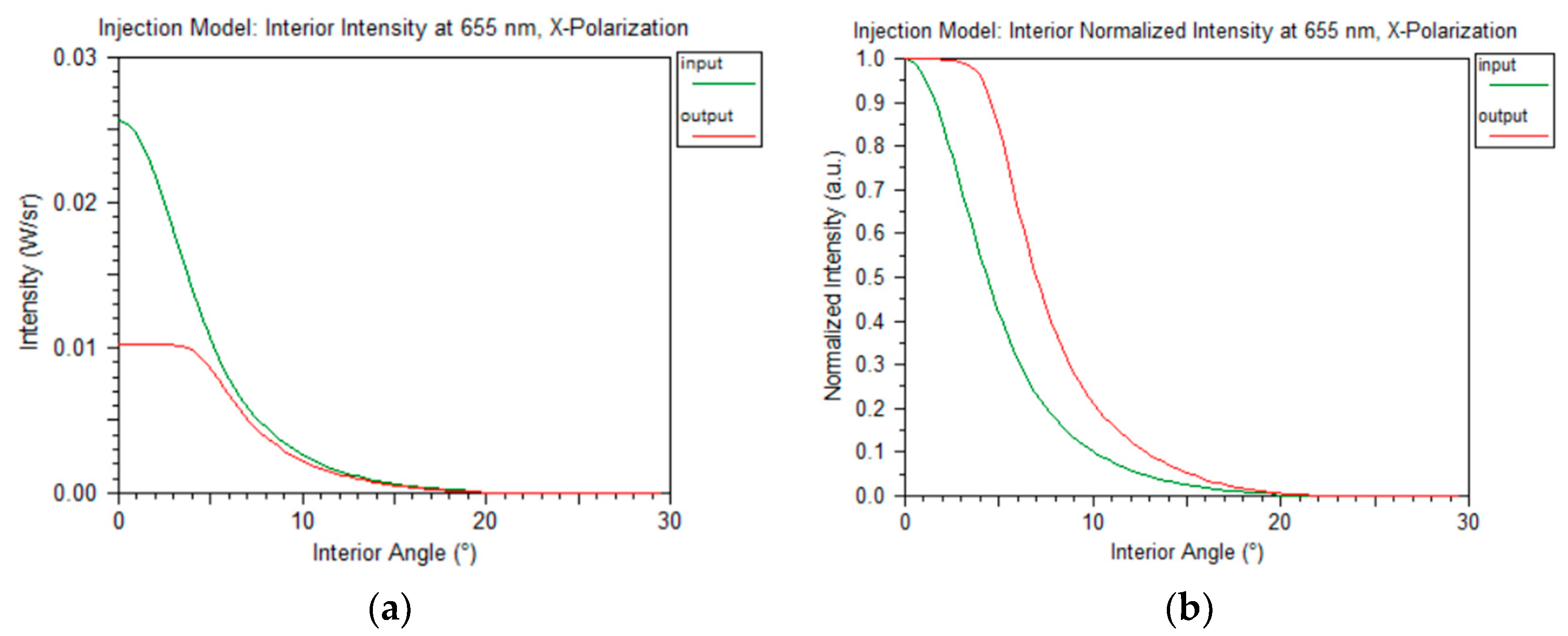
3.3. SI-POF Injection

As described in [29,49], there is strong initial diffusion of power to higher angles at the input of large-core step-index POFs. This strong diffusion cannot be correctly captured by a fit of the Gloge power-flow equation to fiber performance at longer lengths. The strong power diffusion can be modeled via an injection matrix M_inj, in which the output intensity at some angle θ_i is a weighted linear summation of the input powers at all input angles [29]. Using our discretized angles approach, the output intensity as a function of the input intensities can be represented as:

$$p_{out}({\theta }_i,t)={\displaystyle \sum _{j=0}^N{m}_{inj}({\theta }_i,{\theta }_j)\cdot p_{in}({\theta }_j,t)}$$

(14)

where m_inj(θ_i, θ_j) is a coupling coefficient between the input at θ_j and the output at θ_i and t indicates that the signals are in the time domain. If we represent the intensities as vectors P_out(t) = [p_out(θ_i,t)]^T and P_in(t) = [p_in(θ_j,t)]^T, we can also represent this relationship as

$$P_{out}(t)=M_{inj}\cdot P_{in}(t)$$

(15)

where M_inj is the injection matrix with elements m_inj(θ_i, θ_j). M_inj can be derived from measurements, as described in detail in [30,32,49]. An equation equivalent to Equation (15) can be written with the intensity vectors as functions of frequency instead of time:

$$P_{out}(\omega )=M_{inj}\cdot P_{in}(\omega )$$

(16)

In this equation, the injection matrix is the same as that in Equation (15) because it is independent of both time and frequency. As Equations (15) and (16) are formally equal, from now on, we will write the vectors without an explicit dependence on time or frequency when we describe other components to avoid repetition of the time and frequency versions of the equation.

The injection effects in the fiber can also be modeled via an equivalent Gloge model using a fit for α (θ) and D(θ) [20,23,29,30]. In this case, we ignore time-dependence of the Gloge power-flow equation since the injection matrix operates instantaneously. While the Gloge power-flow equation assumes a propagation distance L, this quantity is not meaningful for the injection model. Thus, as shown in [30], because we solve the Gloge equation numerically, we need to specify a fixed number of steps N_z of width Δz to take along the z direction. The choice of Δz is arbitrary and, therefore, it suffices to specify the fiber injection loss factor as a function of angle, the coupling terms D₀ and D₁ of Equation (3) in units of radians² (rather than radians²/m), and the number of steps N_z. The parameters D₂ and σ_d are also specified.

3.4. Connector Modeling

Representing optical signals as intensity functions of the propagation angle makes it possible to implement more computationally efficient models for other components within a large-core POF-based system. Of particular interest is an efficient model that represents connectors between optical fibers, which is essential for modeling a POF-based system. Our connector model follows an approach that is similar to the one used for the SI-POF Injection model discussed above and is based on work presented in [30,50,51]. The key assumption of the model is that for a particular connector, the output intensity at some angle θ_i is a weighted linear summation of the input powers at all input angles. Similar to Equation (10), the output intensity as a function of the input intensities can be represented as:

$$p_{out}({\theta }_i,t)={\displaystyle \sum _{j=0}^N{m}_{conn}({\theta }_i,{\theta }_j)\cdot p_{in}({\theta }_j,t)}$$

(17)

where m_conn(θ_i, θ_j) is a coupling coefficient between the input at θ_j and the output at θ_i. Likewise, if we represent the intensities as vectors P_out and P_in, which can be functions of either time or frequency, we can also represent this relationship as the matrix product:

$$P_{out}=M_{conn}\cdot P_{in}$$

(18)

where M_conn is a matrix with elements m_conn(θ_i, θ_j).

The advantage of this approach is that for any connector arrangement with arbitrary transverse, longitudinal, and angular misalignments, it is possible to measure an appropriate connector matrix which can be used in simulation. As was the case for the Injection model, and discussed in [30], in many cases, it is possible to fit this matrix to the Gloge power-flow equation [20,23,29,30]. In this case, the interpretation of the Gloge power-flow equation is similar to that of the Injection model. We use measured data for α (θ), and a constant value for the power-coupling term D(θ) = D₀.

It is also possible to model lateral and longitudinal misalignments between fibers via analytical expressions [50,51]. This method is based on the hypothesis that each point in the fiber end surface acts as an independent uncorrelated source whose radiation pattern is given by g(θ), as shown in Figure 3a. We assume this function is related to the fiber Far Field Pattern (FFP). To obtain the total radiated intensity at any point in space in cylindrical coordinates R(r, φ, z), the scalar contributions are added from all radiating sources that reach that point (Figure 3b). As all functions involved have circular symmetry, the zero-order Hankel Transform can be used to speed up and simplify calculations. Thus, the light intensity radiated from the end surface of this fiber is given by:

$$R(r,z)=z^2\cdot {\mathrm{H}}^{-1}\left(\frac{a{\mathrm{J}}_1(2\pi a\rho )}{\rho }\cdot G(z\rho )\right)$$

(19)

where ρ is the transformed radial variable, H⁻¹ is the inverse zero-order Hankel transform, J₁(2π a ρ)/ρ is the Airy pattern that is the transform of the circular aperture with radius $a$ used to model the fiber surface, and G(ρ) is the transform of g(r), which is the projection of the radiation pattern. As the radiated intensity has circular symmetry, the explicit dependency on φ has been omitted.

Once the radiated intensity has been obtained, misalignment loss is calculated assuming that the intensity captured by the receiving fiber is the fraction of intensity radiated from the first fiber that overlaps with the core surface of the second fiber, as shown in Figure 4. In this case, the model produces a scalar power-loss factor l_p(r₀, z₀) for a given pair of misalignments [51]. A more flexible approach is to calculate the proportion of light that on exiting the radiating fiber at a given angle of interest in free-space (thus, an external angle) θ_i,ext, is able to reach the receiving fiber. This is equivalent to assuming that each point of the fiber radiates light in a very narrow angular range centered at that angle. Then, instead of a circular pattern, its projection onto a perpendicular plane will be a very narrow ring. The equations to calculate this angular loss function are:

$$R({\theta }_{i,ext},r,z)=2\pi z\tan ({\theta }_{i,ext})a^2{\mathrm{H}}^{-1}\left(\frac{{\mathrm{J}}_1(2\pi a\rho )}{a\rho }\cdot {\mathrm{J}}_0\left(2\pi z\tan ({\theta }_{i,ext})\rho \right)\right)$$

(20a)

$$l_p({\theta }_{i,ext},r_0,z_0)=\{\begin{array}{c}\frac{2{\displaystyle \underset{r_0-a}{\overset{r_0+a}{\int }}{\cos }^{-1}\left(\frac{r_0^2+r^2-a^2}{2r_{0}r}\right)}R({\theta }_{i,ext},r,z_0)rdr}{2\pi {\displaystyle \underset{0}{\overset{\infty }{\int }}R({\theta }_{i,ext},r,z_0)rdr}},\mathrm{if}{r}_0\ge a\\ \frac{2\pi {\displaystyle \underset{0}{\overset{a-r_0}{\int }}R({\theta }_{i,ext},r,z_0)rdr}+2{\displaystyle \underset{a-r_0}{\overset{a+r_0}{\int }}{\cos }^{-1}\left(\frac{r_0^2+r^2-a^2}{2r_{0}r}\right)}R({\theta }_{i,ext},r,z_0)rdr}{2\pi {\displaystyle \underset{0}{\overset{\infty }{\int }}R({\theta }_{i,ext},r,z_0)rdr}},\mathrm{if}{r}_0<a\end{array}$$

(20b)

In the simplest case, we can model the connector using just the analytical model for power loss due to lateral and longitudinal misalignments. However, this will not capture the effects of imperfections in the fiber end facets, nor rapid power diffusion during re-injection of optical power into the second fiber [30]. Thus, the complete model, as described in [50,51], combines both the basic connector matrix, which is used to model the fiber–fiber connection in the absence of any lateral and longitudinal misalignments, along with the analytical misalignment model:

$$P_{out}=M_{misalign}\cdot M_{conn}\cdot P_{in}$$

(21)

where M_misalign is a diagonal matrix whose diagonal elements are calculated from Equation (20b) after conversion from external to internal angles:

$$m_{misalign}({\theta }_i)=l_p({\theta }_i,r_0,z_0)$$

(22)

Equation (21) can be written either in the temporal or in the frequency domain by only introducing the variables of the input and output intensity vectors. The complete connector matrix M_CC is the product of the misalignment matrix M_misalign and the basic connector matrix M_conn, and is the same for the temporal and frequency approaches. Figure 5 shows the connector matrices for several misalignment pairs. The images show how the connector introduces not only attenuation but also diffusion. Misalignments do not introduce further diffusion but can considerably increase attenuation.

3.5. Fiber Bends

In a similar way to connectors, fiber bends can be modeled via a matrix M_bend, or via an equivalent fit of the Gloge power-flow equation [32]. The matrix will depend on the bend radius and also on the bend angle (e.g., a complete turn of 360°, will be different from a right-angle turn of 90°). Once again, the key assumption is that the output intensity at some angle θ_i is a weighted linear summation of the input powers at all input angles. In other words

$$p_{out}({\theta }_i,t)={\displaystyle \sum _{j=0}^N{m}_{bend}({\theta }_i,{\theta }_j)\cdot p_{in}({\theta }_j,t)}$$

(23)

where m_bend (θ_i, θ_j) is a coupling coefficient between the input at θ_j and the output at θ_i. Representing the intensities as vectors P_out and P_in, that can be functions of time or frequency, we can also express this relationship as:

$$P_{out}=M_{bend}\cdot P_{in}$$

(24)

where M_bend is a matrix with elements m_bend (θ_i, θ_j). Furthermore, similar to the Injection and Connector models, and as described in [32], it is possible to fit this matrix to the Gloge power-flow equation [20,23,29,30]. Similarly, the interpretation of the Gloge power-flow equation is the same as that of the Injection and Connector models above. The fiber bend matrix M_bend can be derived from measurements, as described in detail in [32].

3.6. Detector Coupling

In this section, we describe a model that allows for the computationally efficient simulation of optical coupling between the POF and a detector of arbitrary radius in the presence of misalignments. The model can be used to model spatial filtering at the detector and its dependence on the detector radius. It is based on the same equations used in the connector model for modeling the effects of lateral and longitudinal misalignment [50,51]. Using Equation (20a,b), it is possible to determine how much power is actually coupled into the detector, and therefore, determine an angle-dependent loss factor as a function of lateral and longitudinal misalignment, where r₀ is the lateral shift between the fiber axis and the detector center and z₀ is the longitudinal distance of the fiber end to the active area of the photodetector. Accounting for the detector possibly having a radius b that is different from the fiber core radius a, implies replacing a with b in Equation (20b). Thus, we can calculate the power-loss factor as a function of the propagation angle and the two shifts: l_p(θ_i, r₀, z₀). [50,51]. The complete model can be represented as:

$$P_{out}=M_{det}\cdot P_{in}$$

(25)

where P_out is the vector of output intensities, P_in is the vector of input intensities that can be functions of time or frequency, and M_det is a diagonal matrix with diagonal elements m_det(θ_i) calculated as:

$$m_{det}({\theta }_i)=l_p({\theta }_i,r_0,z_0)$$

(26)

4. System Level Modeling: Two-Step and One-Step Approaches

Having provided an overview of the fundamental building blocks needed to model and simulate a large-core POF system, we will now turn our attention to the utilization of the models in POF-based system-level simulations. Conceptually, the modeling approach is the standard hierarchical method in which the building blocks are at the lowest level and the system is at a level above. This allows us to assess the impact of the individual building blocks on the overall system performance. Moreover, the cumulative impact on performance due to propagation through the connected components comprising the system can be quickly evaluated.

Until recently, commercial software packages did not include the capability to model and simulate large-core POFs at the system-level. This led us to develop a two-step simulation approach to meet our immediate need for system-level simulations [34,56]. The first step uses the matrix representation of the components to calculate the output intensity distribution and frequency response of the system being studied. In the second step, system-level simulations are performed by introducing, in any system-level simulation environment, a black box with this frequency response. For example, let us imagine that we have a system consisting of a source, four fiber segments connected by ST connectors, followed by a detector. This scenario is depicted in Figure 6 for the more general case of k fiber segments, where k is a positive integer. As the scheme shows, both the spatial characteristics of the optical source and the photodetector are modeled as was described above and introduced into the POF system (first step). On the other hand, their temporal (frequency) characteristics are introduced in the system-level simulation (second step). Our implementation utilized the frequency-domain approach for the first step where all the components, including the fiber, are modeled with matrices. However, the equivalent time-domain approach would yield the same results.

The system has an optical source in the transceiver that is modeled by its angular intensity in vector form, P_s(ω). The frequency dependence in this vector is flat, as the temporal characteristics of the transmitter are introduced in the second step. As for the fiber segments, they can be modeled with the corresponding propagation matrices M_Li(ω), i = 1, ..., 4, while ST connectors can be modeled by characteristic matrices M_ST. Finally, matrix M_det is the diagonal matrix to account for angles that are not captured in the detector area, as discussed above. As in the case of the transmitter, the frequency response of the receiver and amplifier electronics is introduced in the second step. The optical intensity at the output of the whole POF layout, P_out(ω), can then be calculated as the product of the matrices of every component of the POF link:

$$\begin{array}{ll}{P}_{out}(\omega )& =M_{det}\cdot M_{L4}(\omega )\cdot M_{ST}(\omega )\cdot M_{L3}(\omega )\cdot M_{ST}(\omega )\cdot M_{L2}(\omega )\cdot M_{ST}(\omega )\cdot M_{L1}(\omega )\cdot P_s(\omega )\\ & =M_{det}\cdot F(\omega )\cdot P_s(\omega ),\end{array}$$

(27)

where F(ω) is a single matrix that models the fiber link without the active components and all the individual matrices for each component can be derived as described in the previous sections. Additionally, connector misalignment, fiber bend and injection aspects can be easily accommodated by inserting their corresponding matrices at the appropriate points in Equation (27). Thus, for a given source with a particular spatial distribution, the frequency response of the POF layout can be derived as [29]:

$$H(\omega )=2\pi {\displaystyle \underset{\theta =0}{\overset{{\theta }_{max}}{\int }}{p}_{out}(\theta ,\omega )\sin (\theta )d\theta }$$

(28)

where p_out(θ,ω) is the output intensity vector in the frequency domain, whose discretized version is P_out(ω) from Equation (27), that is shown here as a function of the propagation angle, as well as of the frequency. Therefore, the spatial aspects of the system can be modeled as an equivalent linear system whose frequency response is H(ω).

Once the equivalent frequency response of the POF system has been obtained, the temporal aspects of the system design are introduced during the second step, allowing for the calculation of bit error rate (BER) and eye diagrams using different modulation formats. We implemented the first step using MATLAB^TM [57] and the second used the commercial simulation package OptSim^TM, utilizing its MATLAB co-simulation capability to combine both steps into a single simulation event [58].

While this two-step approach can be quite efficient, especially when the time-domain signal includes a large number of bits (i.e., it provides for a reduced number of components to simulate in the second step), it does have a couple of notable drawbacks: (1) it can be tedious to work with two separate software packages, (2) it only allows access to the transmitted time/frequency domain signal at the input and output of the whole POF system, since the entire system is collapsed into a single black box. To overcome these issues, a one-step approach that integrates the temporal aspects of the signal transmitted through the POF system with the time-space characteristics of the system has been introduced [59,60]. This approach overcomes the first drawback since it fits naturally into a single simulation environment. It overcomes the second drawback since it allows monitoring of the optical intensity, time-domain transmitted signal, or any other desired measurement at inputs and outputs of all the components constituting the POF system. Figure 7 shows schematically the general idea of the one-step approach. The one-step example is shown in the frequency domain, although it will be equivalent to work in the temporal domain. Optical intensity vectors P(ω) at the output of the system components are represented in 2-D according to their dimensions: frequency ω and propagation angle θ.

As can be observed from Figure 7, in the one-step simulation approach, the optical intensity vector at the output of the transmitter, which is propagated throughout the system components, contains not only the spatial but also the frequency properties of the transmitted signal. Therefore, time-domain signals can be easily extracted at any point of the link from the corresponding intensity vectors in order to obtain the desired system-level performance measurements such as BER or eye diagram [61,62]. The derivation from the two-step to the one-step methodology can be done very easily by adding the signal frequency properties as explained in the following. Considering that a data signal s(t) is to be transmitted through a POF link, the output data signal r(t) can be obtained using the inverse Fourier transform and according to the two-step approach as:

$$r(t)={\mathrm{FT}}^{-1}\left(S(\omega )\cdot H(\omega )\right)={\mathrm{FT}}^{-1}\left(S(\omega )\cdot 2\pi {\displaystyle \underset{\theta =0}{\overset{{\theta }_{max}}{\int }}{p}_{out}(\theta ,\omega )\sin (\theta )d\theta }\right)$$

(29)

where S(ω) is the Fourier transform of the input data signal s(t) and H(ω) is the equivalent frequency response of the POF system, that is obtained from Equation (28). Since in Equation (29), the integral is computed in the spatial domain, it can be rewritten as

$$r(t)={\mathrm{FT}}^{-1}\left(2\pi {\displaystyle \underset{\theta =0}{\overset{{\theta }_{max}}{\int }}{p}_{out,sig}(\theta ,\omega )\sin (\theta )d\theta }\right)$$

(30)

where the new variable p_out,sig(θ,ω), that has been introduced, accounts for the output intensity containing both the spatial characteristics of the output signal and its frequency characteristics. This intensity can be calculated taking into account Equations (27) and (29):

$$P_{out,sig}(\omega )=S(\omega )\cdot P_{out}(\omega )=M_{det}\cdot F(\omega )\cdot S(\omega )\cdot P_s(\omega )=M_{det}\cdot F(\omega )\cdot P_{s,sig}(\omega )$$

(31)

so that in the intensity vector P_s,sig(ω) the frequency information of the transmitted data signal has been merged with the spatial information of the optical source and can be propagated in a block-by-block basis to perform system-level simulation of the POF link.

5. Commercial Software

The modeling techniques described so far can be implemented in commercial software packages and this is beginning to happen as POF gains popularity [42,60]. This is very desirable since it makes large-core POF modeling capability available to a potentially large user base. It also lessens the development burden since it allows us to take advantage of sophisticated building blocks included in established commercial packages, which are based on tried-and-tested algorithms and simulation techniques.

5.1. MATLAB/Simulink

As a first stage, the one-step approach has been successfully adapted in a Simulink^TM environment [61]. The POF model formulated in the frequency domain in matrix form can be efficiently implemented in MATLAB, using Simulink as the software user interface and integration engine to build the POF simulation framework. Simulink offers two main simulation modes, denominated sample mode and frame mode, which specify how the schematic building blocks interact and process the signal that propagates throughout the model as the simulation progresses. In sample-based processing, blocks process signals one sample at a time and then propagate the processed sample to the next block. The frame mode accumulates a large number of signal samples constituting a frame. This frame is subsequently processed as a single unit by the model blocks. In our case, the frame-mode has been chosen for introducing the POF models. This simulation mode speeds up simulations significantly. Moreover, since the matrix models are in the frequency domain, working with frames is the natural way to split up the input data signal so that it can undergo a Fourier-transform.

The developed simulation framework consists of a custom Simulink POF library containing blocks that model the fiber and related components, such as sources, connectors, bends etc., described above. Furthermore, due to the particular nature of the signal, custom blocks were designed to perform analysis and plotting functions, such as optical power and 3 dB bandwidth measurement, calculation of the equivalent complex frequency response, group delay and impulse response or representation of the far field pattern [57,60]. The developed blocks interact with the user via dialog boxes to set the parameters that define each model. All these blocks, together with already existing Simulink blocks from the communications blockset, can be put together into a schematic to form the communication system to evaluate. In the developed framework, the default signal passed between blocks is the intensity vector with frequency information of the data, P_s,sig(ω), that has been defined in the description of the one-step simulation methodology.

In this approach, the evolution of the transmitted signal along the POF system is accessible, which enables the evaluation of the optical intensity, the time-domain signal or any other desired measurement at any point of the link. This feature can be of great importance in order to identify the critical path or component in a network. However, a disadvantage of this framework is that Simulink is a general-purpose simulation environment that does not include blocks specific for optical components or optical measurement systems.

5.2. ModeSYS

ModeSYS^TM is a simulation tool that is developed and marketed by Synopsys, Inc. [33]. Over the years, it has been used to model and simulate communication systems based on multimode glass optical fibers, with a primary focus on data communication applications. Unlike SI-POF, these fibers are usually of the graded-index variety made with core diameters of 50 or 62.5 microns, much less than that of SI-POF, which can be as large as 1 mm. Also, the sources are usually in the 850 or 1300 nm wavelength window. This means that, at most, only hundreds of propagating modes are supported by these fibers. Hence, ModeSYS takes the reasonable approach of simulating both the temporal waveform and spatial mode profiles of multimode glass optical fiber systems, thus combining system-level efficiency with device-level representation accuracy. It provides the user with an extensive set of measurement and analysis tools such as the basic signal representation in the time and frequency domains, but also representation of transverse mode profiles, radial power distributions, effective modal bandwidth, differential mode delay, encircled flux, eye diagram and BER.

ModeSYS is able to capture all the guided modes in multimode glass fibers via a signal representation that contains all the detailed spatial mode profiles; however, this representation is not adequate for large-core fibers, where there are millions of propagation modes. In addition, as mentioned before, the strong mode coupling in SI-POF induces power transfer between neighboring modes, which is much higher than in glass multimode fibers. Recently, the ModeSYS framework has been updated to support the modeling and simulation of large-core SI-POF systems based on the modeling techniques described above [33,42]. The approach is essentially an implementation of the one-step approach [57,60], in this case, using the split-step time-domain algorithm for solving the Gloge power flow equation, as opposed to the frequency-domain matrix-based method. Interestingly, the ModeSYS framework provides a method to map the detailed spatial field representation at the POF input to the intensity-vs-angle representation that is assumed by the Gloge power flow equation and is compatible with the model implementations discussed above. To accomplish this, the optical signals with spatial mode profiles at the POF input are first converted into an equivalent intensity representation p(θ, z = 0, t) (where θ is internal angle and z = 0 indicates that we are at the fiber input) via the use of a Fourier-based far-field transformation. The following assumptions are made in carrying out this conversion. First, it is assumed that the input signal originates from free space. Second, it is assumed that the extent of the input beam is fully captured by the fiber core. Third, the far-field transformation is performed using the core index as the medium of propagation. It is also assumed that the fiber rejects any portion of the input that resides at an angle outside of the NA, and therefore, the corresponding launch intensities at these angles are set equal to zero. Finally, the effects of Fresnel reflection at the input are ignored [26]. ModeSYS also supports directly launching an input signal in the intensity-vs-angle domain, allowing the user to specify the angular dependence of the launch intensity via either data files or parameters to set the launch field analytically.

The ModeSYS framework also includes an interface with MATLAB that allows custom models in a simulation to be executed within the MATLAB environment. Through this interface, a user is able to take full advantage of an extensive and proprietary library of digital signal processing (DSP) modeling algorithms that are included with the software package, many of which have been well established in the literature [62]. As a result, sophisticated transmitter and receiver models using a combination of built-in blocks and custom MATLAB components can be implemented. The framework automatically invokes MATLAB as needed and provides for the exchange of propagating signals between the tools. In so doing, advanced modulation formats, along with feedforward and feedback equalization techniques, can be implemented in the MATLAB environment using tried-and-tested algorithms.

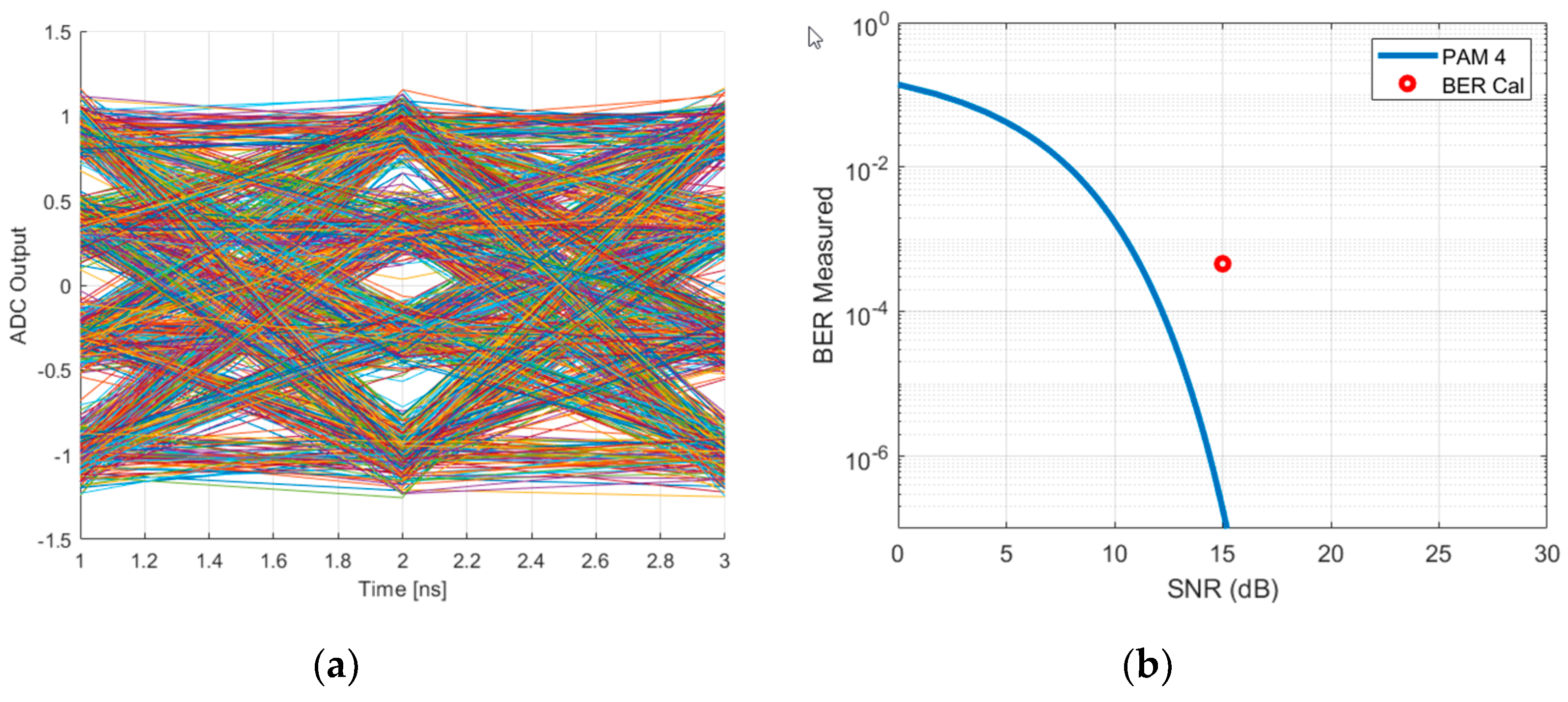
6. System Level Simulation Example: PAM-4 Transmission over Large-Core Plastic Optical Fiber

In this section, we describe an example implemented in the ModeSYS simulation framework based on the component models and system-level modeling techniques discussed above. This example is motivated by real world layouts though it does not attempt to implement the details of any real POF link. The goal is to show an instance that demonstrates the utility of the models for large-core SI-POFs and modeling techniques implemented in the simulation package rather than to create an optimal link design based on the assumed link scenarios and parameters.

Particularly, the example demonstrates how PAM-4 modulation with DSP equalization at the receiver can help overcome the inherent bandwidth limitations of POF at Gb/s data rates for short-distance data interconnects [6,63]. Based partially on work presented in [63,64], Figure 8 illustrates a topology that implements end-to-end 1-Gb/s PAM-4 transmission over 1-mm diameter SI-POF. ModeSYS is used to simulate the fiber using the computationally efficient model based on the Gloge power-flow equation, while MATLAB co-simulation models the transmitter and receiver DSP using functions from the OptSim DSP Library for MATLAB. The transmitter generates an electrical PAM-4 signal with Nyquist pulse shaping and pre-emphasis filtering [65], and the receiver DSP uses a least mean square (LMS) equalization algorithm to recover the transmitted symbols and analytically estimate the BER. A Fiber Injection block is used to model the impact of the strong initial power diffusion at the fiber input [23,29]. The large-core SI-POF parameters used in the simulation are based on extracted model parameters for a 1 mm diameter ESKA-PREMIER GH4001 fiber from Mitsubishi [23]. The fiber injection uses parameters from [30] for the power diffusion, as well as the same angle-dependent loss as that used in the fiber. We would expect that the fiber injection, which tends to spread the power to higher angles, should result in a slower overall system response and reduced system bandwidth. Figure 9a shows the intensity in W/sr (not normalized) as a function of internal angle. Figure 9b shows the normalized version, illustrating the strong power diffusion. Figure 10 depicts the optical eyes at the POF system input and output, showing eye closure due to intermodal dispersion and mode coupling. Figure 11a illustrates the recovered eye diagram after the receiver’s analog-to-digital conversion (ADC) and equalization, which has compensated for the eye closure, while Figure 11b depicts the analytically estimated BER in comparison with an ideal PAM4 reference curve. The BER of 4.6 × 10⁻⁴ is below an FEC threshold of 3.7 × 10⁻³ [66,67]. As described in [63], the supported bit rate for this typical system can be much higher than the 1 Gb/s used in this example. Close to the absolute bandwidth limit, we can also employ a detector coupler to eliminate the higher angle modes at the receiver, thus increasing the bandwidth; however, the resulting power loss in combination with the receiver sensitivity may force other system adjustments to meet the BER specifications.

7. Conclusions

In this paper, we have stressed the need for an accurate comprehensive system-level modeling and simulation framework that allows system designers to explore various design options before building and deploying their particular network. We have presented a review of the fundamental challenges associated with the modeling and simulation of large-core POF-based systems and how we have addressed them at the component and system levels for SI-POF. Specifically, we have described the time domain and the alternative frequency domain approaches to model SI-POF based on the power-flow equation. We then reviewed our approach to modeling various other components, followed by a description of the important system-level modeling considerations. Our approach is rooted in first developing efficient experimentally verified models of the individual components and observed behaviors. Subsequently, the models are used to construct various link or network configurations whose performances are estimated at the system level via typical metrics such as BER and eye diagrams.

We then described our historical approaches to address our need to model POF-based systems since there was a lack of commercial offerings. Thankfully, commercial software packages are now emerging and we have described an approach based on a custom Simulink library and ModeSYS, which is primarily a glass multimode fiber simulation environment which has more recently been adapted to handle large-core POF-based systems.

Our future work will investigate other types of POFs, including various MC SI-POF and GI-POF. The ultimate goal is to again develop reliable models of the components and study them at the system level with an emphasis on high-speed data transmission over these media as we push the limits of POF-based networks. Among other things, the study will naturally involve modulation formats and DSP algorithms for pre- and post-processing at the transmitter and receiver, respectively. Also, the variability of model parameters for the fiber and all the other components will be quantified and more extensively studied at the system level to ensure that the predicted system-level performances are realistic.

References

1. Losada, M.A.; Mateo, J. Short Range (in-building) Systems and Networks: A Chance for Plastic Optical Fibers. In WDM Systems and Networks. Modeling, Simulation, Design and Engineering; Antoniades, N., Ellinas, G., Roudas, I., Eds.; Springer: New York, NY, USA, 2012; pp. 301–323. [Google Scholar]
2. Nespola, A.; Abrate, S.; Gaudino, R.; Zerna, C.; Offenbeck, B.; Weber, N. High-Speed Communications Over Polymer Optical Fibers for In-Building Cabling and Home Networking. IEEE Photonics J. 2010, 2, 347–358. [Google Scholar] [CrossRef]
3. Grzemba, A. MOST: The Automotive Multimedia Network; Franzis Verlag: Munich, Germany, 2011; ISBN 9783645650618. [Google Scholar]
4. Truong, T.K. Commercial airplane fibre optics: Needs, opportunities, challenges. In Proceedings of the 19th International Conference on Plastic Optic Fibres and Application, Tokyo, Japan, 19–21 October 2010; p. DN2-1–M. [Google Scholar]
5. Lee, S.C.J.; Breyer, F.; Randel, S.; van den Boom, H.P.A.; Koonen, A.M.J. High-speed transmission over multimode fiber using discrete multitone modulation. J. Opt. Netw. 2008, 7, 183–196. [Google Scholar]
6. Breyer, F.; Lee, S.C.J.; Randel, S.; Hanik, N. Comparison of OOK- and PAM-4 Modulation for 10 Gbit/s Transmission over up to 300 m Polymer Optical Fiber. In Proceedings of the OFC/NFOEC 2008—2008 Conference on Optical Fiber Communication/National Fiber Optic Engineers Conference, San Diego, CA, USA, 24–28 February 2008; IEEE: Piscataway, NJ, USA, 2008; p. OWB5. [Google Scholar]
7. Zeolla, D.; Nespola, A.; Gaudino, R. Comparison of different modulation formats for 1-Gb/s SI-POF transmission systems. IEEE Photonics Technol. Lett. 2011, 23, 950–952. [Google Scholar] [CrossRef]
8. Loquai, S.; Kruglov, R.; Ziemann, O.; Vinogradov, J.; Bunge, C.-A. 10 Gbit/s over 25 m Plastic Optical Fiber as a Way for Extremely Low-Cost Optical Interconnection. In Proceedings of the Optical Fiber Communication Conference, San Diego, CA, USA, 21–25 March 2010; OSA: Washington, DC, USA, 2010; p. OWA6. [Google Scholar]
9. Loquai, S.; Kruglov, R.; Schmauss, B.; Bunge, C.-A.; Winkler, F.; Ziemann, O.; Hartl, E.; Kupfer, T. Comparison of Modulation Schemes for 10.7 Gb/s Transmission Over Large-Core 1 mm PMMA Polymer Optical Fiber. J. Light. Technol. 2013, 31, 2170–2176. [Google Scholar] [CrossRef]
10. Ziemann, O.; Krauser, J.; Zamzowr, P.E.; Daum, W. Application of Polymer Optical and Glass Fibers. In POF Handbook: Optical Short Range Transmission Systems, 2nd ed.; Springer: Berlin/Heidelberg, Germany, 2008. [Google Scholar]
11. Koike, K.; Koike, Y. Design of Low-Loss Graded-Index Plastic Optical Fiber Based on Partially Fluorinated Methacrylate Polymer. J. Light. Technol. 2009, 27, 41–46. [Google Scholar] [CrossRef]
12. Polley, A.; Kim, J.H.; Decker, P.J.; Ralph, S.E. Statistical Study of Graded-Index Perfluorinated Plastic Optical Fiber. J. Light. Technol. 2011, 29, 305–315. [Google Scholar]
13. Technologies | Perfluorinated GI-POF. Available online: https://chromisfiber.com/technology/why-perfluorinated-gi-pof/ (accessed on 16 June 2019).
14. Aldabaldetreku, G.; Zubia, J.; Durana, G.; Arrue, J. Numerical Implementation of the Ray-Tracing Method in the Propagation of Light Through Multimode Optical Fiber. In POF Modelling: Theory, Measurements and Application; Bunge, C.A., Poisel, H., Eds.; Verlag Books on Demand GmbH: Norderstedt, Germany, 2007. [Google Scholar]
15. Berganza, A.; Aldabaldetreku, G.; Zubia, J.; Durana, G.; Arrue, J. Misalignment Losses in Step-Index Multicore Plastic Optical Fibers. J. Light. Technol. 2013, 31, 2177–2183. [Google Scholar] [CrossRef]
16. Berganza, A.; Aldabaldetreku, G.; Zubia, J.; Durana, G. Ray-tracing analysis of crosstalk in multi-core polymer optical fibers. Opt. Express 2010, 18, 22446–22461. [Google Scholar] [CrossRef]
17. Arrue, J.; Aldabaldetreku, G.; Durana, G.; Zubia, J.; Garces, I.; Jimenez, F. Design of mode scramblers for step-index and graded-index plastic optical fibers. J. Light. Technol. 2005, 23, 1253–1260. [Google Scholar] [CrossRef]
18. Arrue, J.; Kalymnios, D.; Zubia, J.; Fuster, G. Light power behaviour when bending plastic optical fibres. IEE Proc. Optoelectron. 1998, 145, 313–318. [Google Scholar] [CrossRef]
19. Appelt, V.; Bunge, C.; Kruglov, R.; Surkova, G.; Poisel, H.; Zadorin, A. Determination of Mode Coupling Matrix Used by Split-Step Algorithm. In POF Modelling: Theory, Measurements and Application; Bunge, C.A., Poisel, H., Eds.; Verlag Books on Demand GmbH: Norderstedt, Germany, 2007. [Google Scholar]
20. Gloge, D. Optical Power Flow in Multimode Fibers. Bell Syst. Tech. J. 1972, 51, 1767–1783. [Google Scholar] [CrossRef]
21. Breyer, F.; Hanik, N.; Lee, S.; Randel, S. Getting the Impulse Respose of SI-POF by solving the Time-Dependent Power-Flow Equation Using the Crank-Nicholson Scheme. In POF Modelling: Theory, Measurements and Application; Bunge, C.A., Poisel, H., Eds.; Verlag Books on Demand GmbH: Norderstedt, Germany, 2007. [Google Scholar]
22. Djordjevich, A.; Savovic, S. Investigation of mode coupling in step index plastic optical fibers using the power flow equation. IEEE Photonics Technol. Lett. 2000, 12, 1489–1491. [Google Scholar] [CrossRef]
23. Mateo, J.; Losada, M.A.; Garcés, I.; Zubia, J. Global characterization of optical power propagation in step-index plastic optical fibers. Opt. Express 2006, 14, 9028–9035. [Google Scholar] [CrossRef]
24. Stepniak, G.; Siuzdak, J. Modeling of transmission characteristics in step-index polymer optical fiber using the matrix exponential method. Appl. Opt. 2018, 57, 9203–9207. [Google Scholar] [CrossRef]
25. Jiang, G.; Shi, R.F.; Garito, A.F. Mode coupling and equilibrium mode distribution conditions in plastic optical fibers. IEEE Photonics Technol. Lett. 1997, 9, 1128–1130. [Google Scholar] [CrossRef]
26. Zubia, J.; Durana, G.; Aldabaldetreku, G.; Arrue, J.; Losada, M.A.; Lopez-Higuera, M. New method to calculate mode conversion coefficients in si multimode optical fibers. J. Light. Technol. 2003, 21, 776–781. [Google Scholar] [CrossRef]
27. Rousseau, M.; Jeunhomme, L. Numerical Solution of the Coupled-Power Equation in Step-Index Optical Fibers. IEEE Trans. Microw. Theory Tech. 1977, 25, 577–585. [Google Scholar] [CrossRef]
28. Djordjevich, A.; Savović, S. Numerical solution of the power flow equation in step-index plastic optical fibers. J. Opt. Soc. Am. B 2004, 21, 1437–1438. [Google Scholar] [CrossRef]
29. Mateo, J.; Losada, M.A.; Zubia, J. Frequency response in step index plastic optical fibers obtained from the generalized power flow equation. Opt. Express 2009, 17, 2850–2860. [Google Scholar] [CrossRef]
30. Esteban, A.; Losada, M.A.; Mateo, J.; Antoniades, N.; López, A.; Zubia, J. Effects of connectors in si-pofs transmission properties studied in a matrix propagation framework. In Proceedings of the 20th International Conference on Plastic Optical Fibres and Applications, Bilbao, Spain, 14–16 September 2011; pp. 341–346. [Google Scholar]
31. Losada, M.A.; Mateo, J.; Martínez-Muro, J.J. Assessment of the impact of localized disturbances on SI-POF transmission using a matrix propagation model. J. Opt. 2011, 13, 055406. [Google Scholar] [CrossRef]
32. Losada, M.A.; López, A.; Mateo, J. Attenuation and diffusion produced by small-radius curvatures in POFs. Opt. Express 2016, 24, 15710. [Google Scholar] [CrossRef]
33. ModeSYSTM–Multimode Optical Communication Systems. Available online: https://www.synopsys.com/optical-solutions/rsoft/system-network-modesys.html (accessed on 15 June 2019).
34. Richards, D.H.; Losada, M.A.; Antoniades, N.; Lopez, A.; Mateo, J.; Jiang, X.; Madamopoulos, N. Modeling Methodology for Engineering SI-POF and Connectors in an Avionics System. J. Light. Technol. 2013, 31, 468–475. [Google Scholar] [CrossRef]
35. Lopez, A.; Jiang, X.; Losada, M.A.; Mateo, J.; Richards, D.; Madamopoulos, N.; Antoniades, N. Temperature sensitivity of POF links for avionics applications. In Proceedings of the 2017 19th International Conference on Transparent Optical Networks (ICTON), Girona, Spain, 2–6 July 2017; IEEE: Piscataway, NJ, USA, 2017. [Google Scholar]
36. Pujols, N.; Losada, M.Á.; Mateo, J.; López, A.; Richards, D. A POF Model for Short Fiber Segments in Avionics Applications. In Proceedings of the 2016 18th International Conference on Transparent Optical Networks (ICTON), Trento, Italy, 10–14 July 2016; IEEE: Piscataway, NJ, USA, 2016. [Google Scholar]
37. Raptis, N.; Grivas, E.; Pikasis, E.; Syvridis, D. Space-time block code based MIMO encoding for large core step index plastic optical fiber transmission systems. Opt. Express 2011, 19, 10336–10350. [Google Scholar] [CrossRef]
38. Lopez, A.; Losada, A.; Mateo, J.; Zubia, J. On the Variability of Launching and Detection in POF Transmission Systems. In Proceedings of the 2018 20th International Conference on Transparent Optical Networks (ICTON), Bucharest, Romania, 1–5 July 2018; IEEE: Piscataway, NJ, USA, 2018. [Google Scholar]
39. Werzinger, S.; Bunge, C.A.; Loquai, S.; Ziemann, O. An Analytic Connector Loss Model for Step-Index Polymer Optical Fiber Links. J. Light. Technol. 2013, 31, 2769–2776. [Google Scholar] [CrossRef]
40. Werzinger, S.; Bunge, C.A. Statistical analysis of intrinsic and extrinsic coupling losses for step-index polymer optical fibers. Opt. Express 2015, 23, 22318–22329. [Google Scholar] [CrossRef]
41. IEEE 802.3bv-2017—IEEE Standard for Ethernet Amendment 9: Physical Layer Specifications and Management Parameters for 1000 Mb/s Operation Over Plastic Optical Fiber. Available online: https://standards.ieee.org/standard/802_3bv-2017.html (accessed on 13 June 2019).
42. Mena, P.V.; Ghillino, E.; Richards, D.; Hyuga, S.; Nakai, M.; Kagami, M.; Scarmozzino, R. Using system simulation to evaluate design choices for automotive ethernet over plastic optical fiber. In Proceedings of the SPIE 10560, Metro and Data Center Optical Networks and Short-Reach Links, San Francisco, CA, USA, 30–31 January 2018; Glick, M., Srivastava, A.K., Akasaka, Y., Eds.; SPIE: Bellingham, WA, USA, 2018; Volume 10560, p. 17. [Google Scholar]
43. Lopez, A.; Losada, A.; Richards, D.; Mateo, J.; Jiang, X.; Antoniades, N. Statistical Approach for Modeling Connectors in SI-POF Avionics Systems. In Proceedings of the 2019 International Conference of Transparent Optical Networks (ICTON), Angers, France, 9–13 July 2019. [Google Scholar]
44. Cherian, S.; Spangenberg, H.; Caspary, R. Investigation on Harsh Environmental Effects on polymer Fiber Optic link for Aircraft Systems; Kazemi, A.A., Kress, B.C., Mendoza, E.A., Eds.; International Society for Optics and Photonics: Bellingham, WA, USA, 2014; Volume 9202, p. 92020I. [Google Scholar]
45. Poisel, H. Optical fibers for adverse environments. In Proceedings of the 12th International. Conference on Plastic Optical. Fibers, Seattle, WA, USA, 14–17 September 2003; pp. 10–15. [Google Scholar]
46. Chen, L.W.; Lu, W.H.; Chen, Y.C. An investigation into power attenuations in deformed polymer optical fibers under high temperature conditions. Opt. Commun. 2009, 282, 1135–1140. [Google Scholar] [CrossRef]
47. Savovic, S.; Djordjevich, A. Mode Coupling in Plastic-Clad Silica Fibers and Organic Glass-Clad PMMA Fibers. J. Light. Technol. 2014, 32, 1290–1294. [Google Scholar] [CrossRef]
48. Tao, R.; Hayashi, T.; Kagami, M.; Kobayashi, S.; Yasukawa, M.; Yang, H.; Robinson, D.; Baghsiahi, H.; Fernández, F.A.; Selviah, D.R. Equilibrium modal power distribution measurement of step-index hard plastic cladding and graded-index silica multimode fibers. In Proceedings of the SPIE 9368, Optical Interconnects XV, San Francisco, CA, USA, 9–11 February 2015; Schröder, H., Chen, R.T., Eds.; SPIE: Bellingham, WA, USA, 2015; p. 93680N. [Google Scholar]
49. Losada, M.A.; Mateo, J.; Serena, L. Analysis of Propagation Properties of Step Index Plastic Optical Fibers At Non-Stationary Conditions. In Proceedings of the 16th International Conference on Plastic Optical Fibres and Applications, Turin, Italy, 10–12 September 2007; pp. 299–302. [Google Scholar]
50. Mateo, J.; Losada, M.A.; Antoniades, N.; Richards, D.; Lopez, A.; Zubia, J. Connector misalignment matrix model. In Proceedings of the 21st International Conference on Plastic Optical Fibres and Applications, Atlanta GA, USA, 10–12 September 2012; pp. 90–95. [Google Scholar]
51. Mateo, J.; Losada, M.A.; López, A. POF misalignment model based on the calculation of the radiation pattern using the Hankel transform. Opt. Express 2015, 23, 8061–8072. [Google Scholar] [CrossRef] [Green Version]
52. Gloge, D. Impulse Response of Clad Optical Multimode Fibers. Bell Syst. Tech. J. 1973, 52, 801–816. [Google Scholar] [CrossRef]
53. Yevick, D.; Stoltz, B. Effect of mode coupling on the total pulse response of perturbed optical fibers. Appl. Opt. 1983, 22, 1010–1015. [Google Scholar] [CrossRef]
54. Stoltz, B.; Yevick, D. Influence of mode coupling on differential mode delay. Appl. Opt. 1983, 22, 2349–2355. [Google Scholar] [CrossRef]
55. Press, W.H.; Teukolsky, S.A.; Vetterling, W.T.; Flannery, B.P. Numerical Recipes in C: The Art of Scientific Computing; Cambridge University Press: Cambridge, UK, 1992; ISBN 9780521431088. [Google Scholar]
56. Antoniades, N.; Losada, M.A.; Mateo, J.; Richards, D.; Truong, T.K.; Jiang, X.; Madamopoulos, N. Modeling and characterization of si-pof and connectors for use in an avionics system. In Proceedings of the 20th International Conference on Plastic Optical Fibres and Applications, Bilboa, Spain, 14–16 September 2011; pp. 105–110. [Google Scholar]
57. MATLAB—MathWorks—MATLAB & Simulink. Available online: https://www.mathworks.com/products/matlab.html (accessed on 14 June 2019).
58. OptSim—OptSim Product Overview | RSoft Products. Available online: https://www.synopsys.com/optical-solutions/rsoft/system-network-optsim.html (accessed on 14 June 2019).
59. Lopez, A.; Losada, M.A.; Mateo, J.J. Simulation framework for POF-based communication systems. In Proceedings of the 2015 17th International Conference on Transparent Optical Networks (ICTON), Budapest, Hungary, 5–9 July 2015; IEEE: Piscataway, NJ, USA, 2015; Volume 2015, p. Mo.D5.4. [Google Scholar]
60. Alcoceba, A.; Lopez, A.; Losada, M.A.A.; Mateo, J.; Vazquez, C.; López, A.; Losada, M.A.A.; Mateo, J.; Vázquez, C. Building a Simulation Framework for POF Data Links. In Proceedings of the 24th International Conference on Plastic Optical Fibers, Nuremberg, Germany, 22–24 September 2015. [Google Scholar]
61. Simulink—Simulation and Model-Based Design—MATLAB & Simulink. Available online: https://www.mathworks.com/products/simulink.html (accessed on 15 June 2019).
62. Bosco, G.; Curri, V.; Carena, A.; Poggiolini, P.; Forghieri, F. On the Performance of Nyquist-WDM Terabit Superchannels Based on PM-BPSK, PM-QPSK, PM-8QAM or PM-16QAM Subcarriers. J. Light. Technol. 2011, 29, 53–61. [Google Scholar] [CrossRef]
63. Kruglov, R.; Loquai, S.; Bunge, C.-A.; Schueppert, M.; Vinogradov, J.; Ziemann, O. Comparison of PAM and CAP Modulation Schemes for Data Transmission Over SI-POF. IEEE Photonics Technol. Lett. 2013, 25, 2293–2296. [Google Scholar] [CrossRef]
64. Kruglov, R.; Vinogradov, J.; Loquai, S.; Ziemann, O.; Bunge, C.-A.; Hager, T.; Strauss, U. 21.4 Gb/s Discrete Multitone Transmission over 50-m SI-POF employing 6-channel WDM. In Proceedings of the Optical Fiber Communication Conference, San Francisco, CA, USA, 9–13 March 2014; OSA: Washington, DC, USA, 2014; p. Th2A.2. [Google Scholar]
65. Erkilinc, M.S.; Thakur, M.P.; Pachnicke, S.; Griesser, H.; Mitchell, J.; Thomsen, B.C.; Bayvel, P.; Killey, R.I. Spectrally Efficient WDM Nyquist Pulse-Shaped Subcarrier Modulation Using a Dual-Drive Mach–Zehnder Modulator and Direct Detection. J. Light. Technol. 2016, 34, 1158–1165. [Google Scholar] [CrossRef]
66. Karinou, F.; Prodaniuc, C.; Stojanovic, N.; Ortsiefer, M.; Daly, A.; Hohenleitner, R.; Kogel, B.; Neumeyr, C. Directly PAM-4 Modulated 1530-nm VCSEL Enabling 56 Gb/s/λ Data-Center Interconnects. IEEE Photonics Technol. Lett. 2015, 27, 1872–1875. [Google Scholar] [CrossRef]
67. Yekani, A.; Chagnon, M.; Park, C.S.; Poulin, M.; Plant, D.V.; Rusch, L.A. Experimental comparison of PAM vs. DMT using an O-band silicon photonic modulator at different propagation distances. In Proceedings of the 2015 European Conference on Optical Communication (ECOC), Valencia, Spain, 27 September–1 October 2015. [Google Scholar]
Figure 1. (a) Graphical representation of the calculation of the optical intensity at the output of the fiber as a function of the input intensity; (b) absolute values of the fiber matrices for a 25 m step-index plastic optical fiber (SI-POF) at different values of ω that correspond to frequencies of 0, 0.5 and 1 GHz.
Photonics 06 00088 g001
Figure 2. Normalized intensities (a) and encircled angular flux (EAFs) (b) as a function of the width of the Gaussian intensity profile as emitted by the source (L = 0 m) and at the output of a 150 m SI-POF.
Photonics 06 00088 g002
Figure 3. (a) Point A in the fiber end surface has a radiation pattern given by g(θ) and (b) each point in the fiber end surface (A, B, C, D, etc.) acts as an independent uncorrelated source.
Photonics 06 00088 g003
Figure 4. The radiated pattern R(r0, z0) is integrated over the receiving fiber end surface to obtain misalignment loss.
Photonics 06 00088 g004
Figure 5. Basic connector matrix with no lateral or longitudinal misalignment (center up) and examples of connector matrices with various combined misalignments. Values of the misalignment are given in mm.
Photonics 06 00088 g005
Figure 6. System-level simulation of a POF system according to the two-step methodology.
Photonics 06 00088 g006
Figure 7. System-level simulation of a POF link according to the one-step methodology.
Photonics 06 00088 g007
Figure 8. Topology for simulating PAM4 transmission over SI-POF.
Photonics 06 00088 g008
Figure 9. Injection model intensity profile at input and output: not normalized (a) and normalized (b), showing the strong initial power diffusion from lower to higher angles.
Photonics 06 00088 g009
Figure 10. Simulated POF input (a) and output (b) eyes, showing the effects of intermodal dispersion and mode coupling.
Photonics 06 00088 g010
Figure 11. (a) Equalized eye at the receiver demonstrating compensation of eye closure. (b) Analytical BER estimate in comparison to an ideal reference curve.
Photonics 06 00088 g011