Ultra-Wideband WDM Optical Network Optimization

Abstract

Ultra-wideband wavelength division multiplexed networks enable operators to use more effectively the bandwidth offered by a single fiber pair and thus make significant savings, both in operational and capital expenditures. The main objective of this study is to minimize optical node resources, such as transponders, multiplexers and wavelength selective switches, needed to provide and maintain high quality of network services, in ultra-wideband wavelength division multiplexed networks, at low cost. A model based on integer programming is proposed, which includes a detailed description of optical network nodal resources. The developed optimization tools are used to study the ultra-wideband wavelength division multiplexed network performance when compared with the traditional C-band wavelength division multiplexed networks. The analysis is carried out for realistic networks of different dimensions and traffic demand sets.

1. Introduction

Optical networks based on Wavelength Division Multiplexing (WDM) technology that operate within the C-band are near the limit of their capacity. New ideas are hence explored to increase the data transmission rates in WDM networks. These include especially the use of transmission wavelengths adjacent to the C-band, i.e., the Ultra Wideband WDM (UW-WDM) systems, and systems that rely on use of optical fibers with a larger number of cores, i.e., Space Division Multiplexing (SDM) systems. Of these two approaches to increasing the telecommunication network transport capacity, the former one is at the moment much nearer to practical implementation since the latter is linked with the need to deploy multicore fibers. Hence, the analysis of routing in UW-WDM systems is the main subject of this contribution.

From the network operator point of view, the ever-increasing demand for high-speed data services translates into the need to continually upgrade the networks to increase the data transmission rate per optical fiber. In currently deployed optical networks, which are based on single core fibers, the data transmission rate can be increased by using either a larger per-channel bit rate or by increasing the number of available channels within a certain transmission spectrum. Furthermore, an increase in the transmission rate can be achieved by using transponders with advanced modulation formats or by adding polarization multiplexing. All these means of increasing the data transmission rate within the C-band will reach soon the limits set by the information theory and the physics of the optical pulse propagation within silica glass optical fibers. Thus, the WDM network equipment providers have to expand the system capacity by reaching out to other segments of the optical spectrum that are available in silica glass optical fibers, i.e., the S-band and L-band.

Existing fiber optic networks that operate in C-band (1530 nm to 1565 nm) typically support up to 96 channels of 50 GHz bandwidth. The selection of the C-band for optical long-haul communications was justified by the presence of low light attenuation in silica glass fiber and by the availability of high quality, low cost erbium ion doped fiber amplifiers (EDFAs) pumped by semiconductor lasers. One option for gaining additional capacity in C-band WDM systems is to use flexible grid, which enables provisioning flexible size WDM channels (flexible grid) with bandwidth as small as 12.5 GHz and the carrier wavelength step of 6.25 GHz. This allows for a more effective use of the available bandwidth within the C-band, mainly by effectively reducing the guard bands. However, once all transmission channels of the C-band are filled, the only way of further increasing the link capacity is through adding on a new pair of fibers. Since many backbone network service providers lease fiber pairs, adding a new fiber pair may translate into a significant increase of the network operating cost and thus may prove prohibitively expensive. Considering that the fiber lease prices are usually quoted per fiber length unit [1], a significant increase of operational costs may adversely affect further network expansion particularly in the network sections that use long routes.

An alternative approach that provides additional capacity to the optic network operators is the use of L-band (1565 nm to 1625 nm). The throughput obtained using both C and L bands is significantly larger than that obtained using C band only [2,3], and recently it was shown to exceed 100 Tb/s [4], reaching even 150 Tb/s when C, L, and S bands are used [5,6,7,8,9]. The L-band shares the main characteristics with the C-band, i.e., low attenuation in silica glass fibers and availability of good quality and cost effective EDFAs pumped by semiconductor lasers. The network equipment providers already offer solutions that allow taking advantage of the C-band and L-band in one fiber pair. Such an UW-WDM solution provides up to 192 50 GHz bands instead of 96 channels available in the traditional C-band WDM systems. Thus, in this paper, we explore the advantages of UW-WDM system using C + L-band when compared with the traditional C-band-based WDM system.

The currently available UW-WDM routing architecture provides channels with minimum bandwidth of 12.5 GHz and the carrier wavelength step of 6.25 GHz (flexible grid) over the C + L bands along with colorless, directionless and contentionless operation (CDC-F). In modern optical WDM networks based on CDC-F Reconfigurable Optical Add Drop Multiplexer (ROADM) operating within C + L band wavelength routing improves to the point whereby practically every segment of the available bandwidth can be accessed by a transponder with an almost arbitrary carrier wavelength and operating bandwidth. Thus, the overall network flexibility increases and potentially reduces the operational costs. CDC-F ROADMs allow for simple adding, dropping and express routing traffic through network nodes and hence offer benefits such as simple planning, simple and robust bandwidth use and low cost network maintenance since CDC-F ROADMs conform with Software Defined Network (SDN) paradigm. Finally, the advantages of the CDC-F ROADM structure enable operators to offer a flexible service, which may translate into a reduction of Operational Expenditure (OpEx) and Capital Expenditure (CapEx) when compared with other solutions [10,11].

During the last decade, the attention of the telecommunication community was concentrated on Routing and Wavelength Assignment (RWA) and Routing and Spectrum Allocation (RSA) problems. Both problems mainly concern the C-band. Consequently, numerous exact and heuristic methods are now available to solve RWA and RSA problems in static [12,13,14,15] and dynamic [16,17,18] environments. However, only recently has the relevance of the ultra wideband networks been considered. This study concentrates on the optimization of UW-WDM networks. The problem is formulated using Mixed Integer Programming (MIP). A comparative study of UW-WDM and classical C-band WDM network is performed. Network topologies used in the simulations are realistic and representative for optical DWDM networks for selected countries [19]. Traffic demands are typical for DWDM networks and are represented using a traffic matrix.

The rest of the paper is organized as follows. In Section 2, the mathematical background relevant to the applied optimizing procedures is provided. In Section 3, a discussion of the results is provided, which is followed by a concise summary given in the last section.

2. Problem Formulation

In this section, UW-WDM network optimization problem is formulated using MIP. For this purpose, the following sets are defined:

$\mathcal{N}$

set of all nodes

$\mathcal{T}$

set of transponders

$\mathcal{S}$

set of frequency slices

$\mathcal{E}$

set of edges

${\mathcal{P}}_{(n,n^{\prime })}$

set of paths between nodes $n,n^{\prime }\in \mathcal{N}$; $p\subseteq \mathcal{E}$

$\mathcal{B}$

set of bands

${\mathcal{S}}_b$

set of frequency slices used by band $b\in \mathcal{B}$; ${\mathcal{S}}_b\subseteq \mathcal{S}$; ${\displaystyle \bigcup _{b\in \mathcal{B}}}{\mathcal{S}}_b=\mathcal{S}$

${\mathcal{S}}_t$

set of frequency slices that can be used as starting slices for transponder $t\in \mathcal{T}$; ${\mathcal{S}}_t\subseteq \mathcal{S}$

The following objective cost function is optimized using an IP algorithm subject to the listed below constraints:

$$min\sum _{b\in \mathcal{B}}(\xi \left(b\right)\sum _{e\in \mathcal{E}}{y}_{be}+\sum _{t\in \mathcal{T}}\xi (t,b)\sum _{n,n^{\prime }\in \mathcal{N}}\sum _{p\in {\mathcal{P}}_{(n,n^{\prime })}}\sum _{s\in {\mathcal{S}}_t}{x}_{tn{n}^{\prime }ps})$$

(1)

where, $\xi \left(b\right)$ is a cost of using band b at a single edge (equipment like: ETFAs, preamplifiers, and boosters are considered), $y_{be}$ is a binary variable, equals 1 if band b is used on edge e and 0 otherwise, $\xi (t,b)$ is a cost of using a pair of transponders t in band b and $x_{tn{n}^{\prime }ps}$ is a binary variable that equals 1 if transponders t are installed between node n and node $n^{\prime }$, routed on path p, and starting on frequency slice $s\in {\mathcal{S}}_t$ and 0 otherwise.

In the cost model ETFAs, preamplifiers, boosters, and transponders are included but not WSSs, ILAs, and filters since the latter devices are not a subject of optimization.

In the model the following three constraints were included:

$$\sum _{t\in \mathcal{T}}\sum _{p\in {\mathcal{P}}_{(n,n^{\prime })}}\sum _{s\in {\mathcal{S}}_t}v\left(t\right)x_{tn{n}^{\prime }ps}\ge d(n,n^{\prime })\forall n,n^{\prime }\in \mathcal{N}$$

(2)

where, $v\left(t\right)$ is a bitrate provided by transponder t and $d(n,n^{\prime })$ is a bitrate demanded from node n to node $n^{\prime }$.

$$\begin{array}{c}\hfill x_{tn{n}^{\prime }ps}h\nu \left(b\right)c\left(t\right)\Delta \left(t\right)\sum _{e\in \mathcal{E}}w(n,n^{\prime },p,e)·(f\left(e\right)(e^{\frac{\mu \left(s\right)l\left(e\right)}{1+f\left(e\right)}}+V-2)+(e^{\frac{\mu \left(s\right)l\left(e\right)}{1+f\left(e\right)}}+W-2))\le P_0\\ \hfill \forall t\in \mathcal{T},\forall n,n^{\prime }\in \mathcal{N},\forall p\in {\mathcal{P}}_{(n,n^{\prime })},\forall b\in \mathcal{B},\forall s\in {\mathcal{S}}_b\end{array}$$

(3)

where, h is the Planck constant equal to $6.62607004·{10}^{-34} {\mathrm{m}}^2 \mathrm{k}\mathrm{g}/\mathrm{s}$, $\nu \left(b\right)$ is a frequency of band b, $c\left(t\right)$ is an OSNR of transponder t, which was calculated using the standard formula, c.f. [20,21,22,23]. $\Delta \left(t\right)$ is the bandwidth used by a transponder t, $f\left(e\right)$ is several In-Line Amplifiers (ILAs) evenly distributed over edge e to re-amplify the signal in order to prevent OSNR from dropping to a very small value, $\mu \left(s\right)$ is a loss per km using slice s, $l\left(e\right)$ is a length of edge e, V and W is the maximum gain of ILA in C and L band, respectively. Both amplifiers compensate for the nodal loss, while the transmitter output power for a single WDM channel is assumed to be equal to 1 mW and is represented by $P_0$. Finally, a constraint is added for avoiding duplicate allocation of the same wavelength in an edge:

$$\sum _{t\in \mathcal{T}}\sum _{n,n^{\prime }\in \mathcal{N}}\sum _{p\in {\mathcal{P}}_{(n,n^{\prime })}}\sum _{s\in {\mathcal{S}}_t}w(n,n^{\prime },p,e)u(t,s,s^{\prime })·x_{tn{n}^{\prime }ps}\le y_{be}\forall e\in \mathcal{E},\forall b\in \mathcal{B},\forall s^{\prime }\in {\mathcal{S}}_b$$

(4)

where, $w(n,n^{\prime },p,e)$ is a binary constant that equals 1 if a path p between nodes n and $n^{\prime }$ uses edges e and 0 otherwise, $u(t,s,s^{\prime })$ is a binary constant that equals 1 if transponder t using bandwidth starting at frequency slice s also uses frequency slice $s^{\prime }$ and 0 otherwise.

The subject of minimization is the cost of installed amplifiers and transponders in (1). Constraints (2) ensure that all demands are satisfied. Constraints (3) ensure that all installed transponders are routed in such a way that their power budgets are not exceeded. Notice that these constraints can be precalculated and reduced to $x_{tn{n}^{\prime }ps}=0$ for some combinations of indices and removed for other combinations. Finally, (4) ensure that using a band results in installing appropriate amplifiers. Notice that these constraints also ensure that each frequency slice at each edge is not used more than once. It is noted that the constraints included do not allow for considering nonlinear interactions and resulting signal impairments.

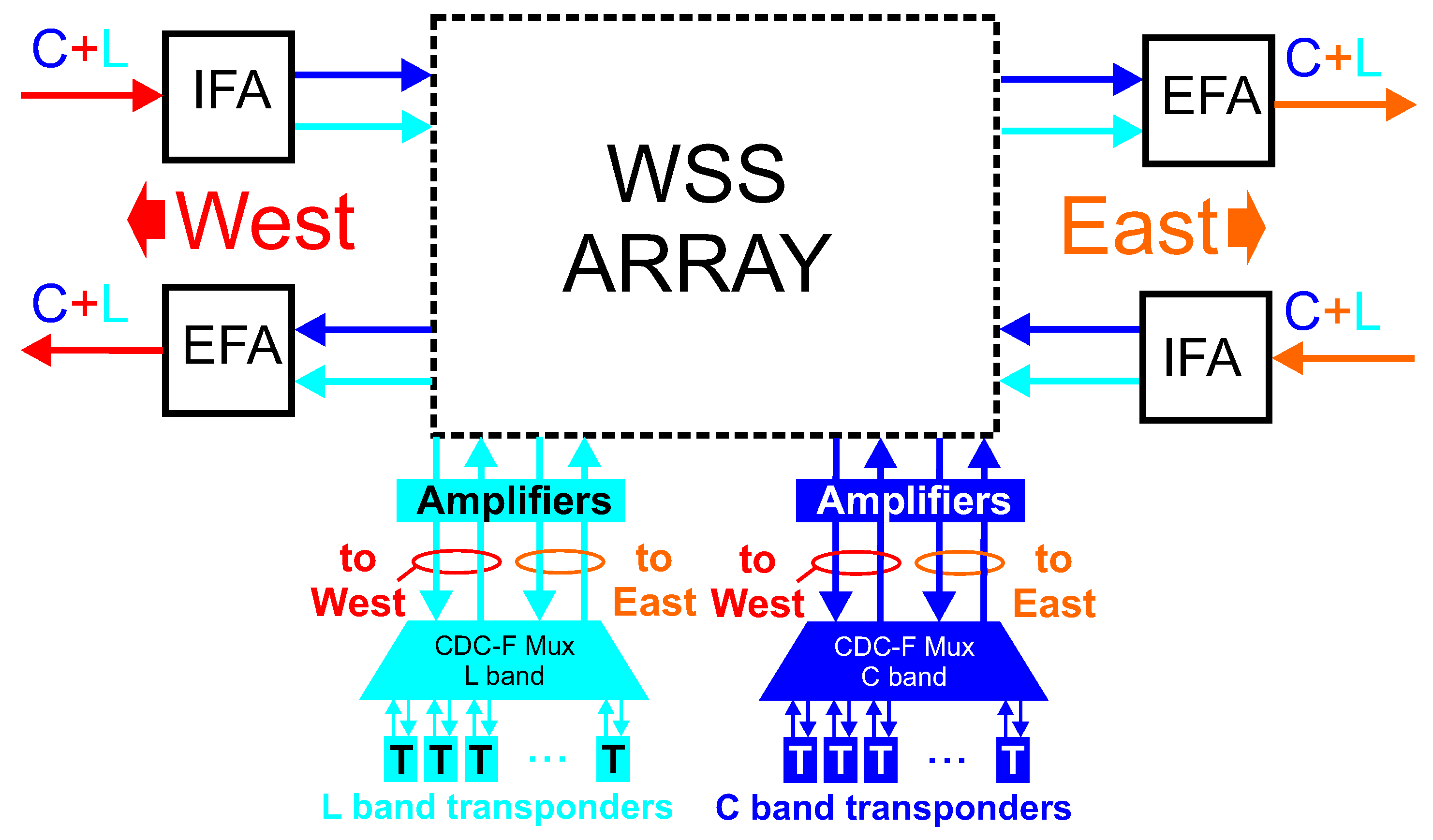
Figure 1 shows a schematic diagram of a two dimensional CDC-F Reconfigurable Optical Add Drop Multiplexer (ROADM) architecture for an UW-WDM optical network operating within C + L-band that was assumed while performing optimization. Higher dimensional nodes are arranged in an analogous manner.

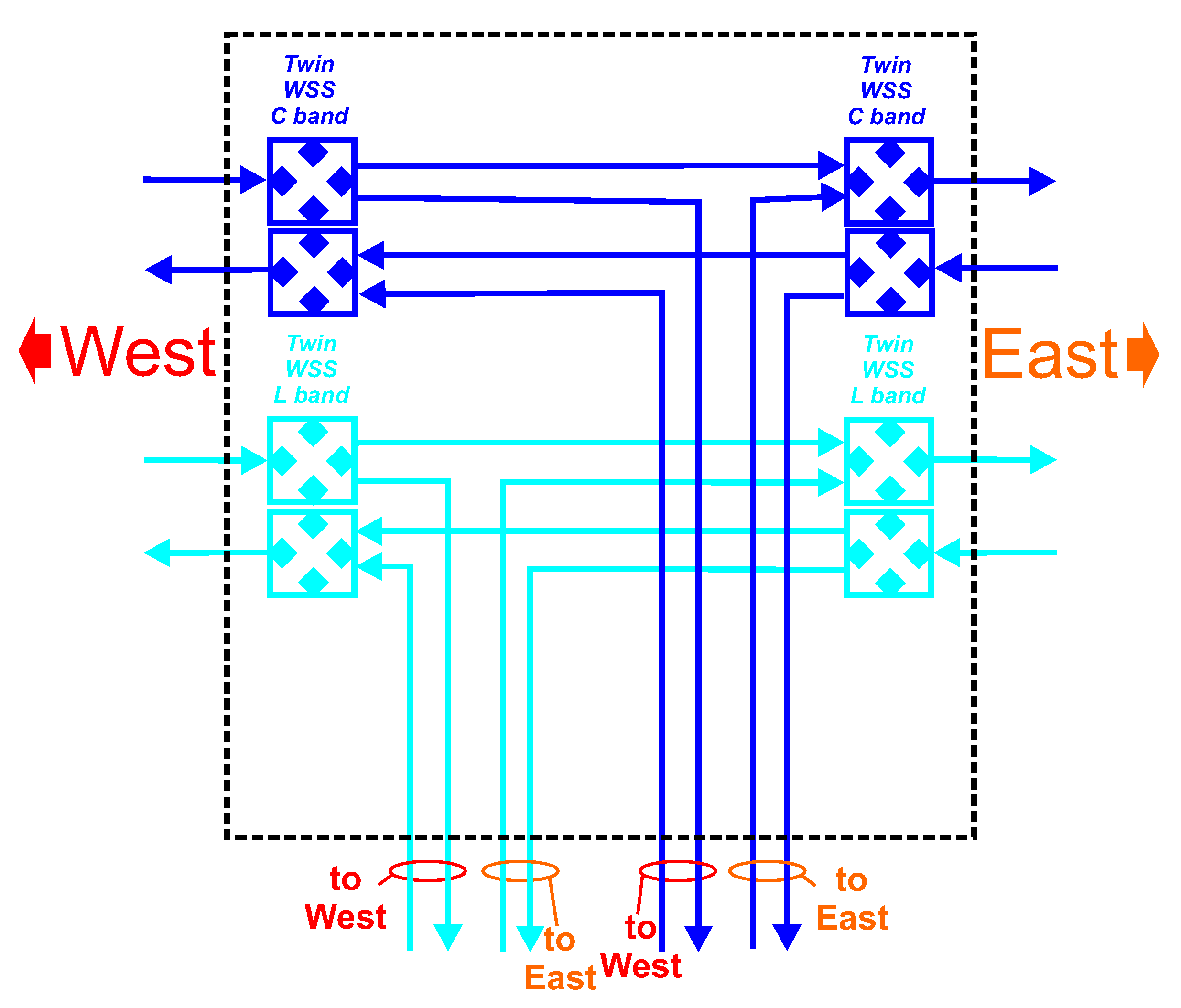
In Figure 1 Ingress Fiber Amplifier (IFA) amplifies the signal entering the ROADM from a transmission line. In IFA the C and L band are separated using a C/L band splitter and the C and L band signals are fed separately to C and L band fiber amplifiers. After amplification the C and L band signals are fed separately to Wavelength Selective Switch (WSS) array. The inner structure of the WSS array is shown in Figure 2.

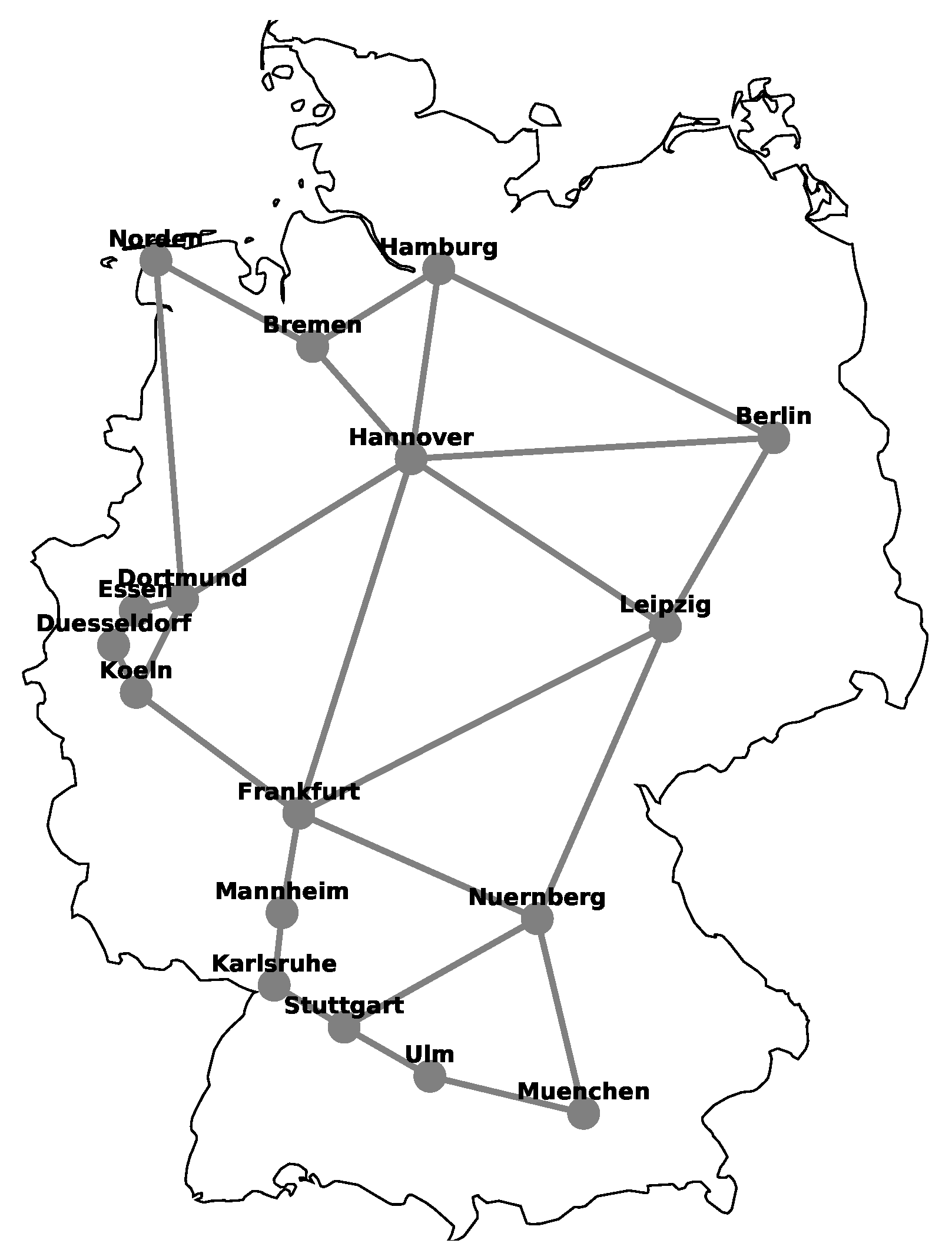
The C- and L-band signals are handled separately by C- and L-band WSSs that connect the signals entering and leaving the node with the CDC-F multiplexers and transponders (Figure 1). The signals leaving the node are boosted by the Egress Fiber Amplifiers (EFAs). In an EFA similarly as for IFA and C-band and L-band signals are amplified separately and combined together using a C/L band combiner before being sent into the transmission line. The overall network node attenuation for transit traffic and for add-drop channels was assumed to be equal to 15 dB and independent of the node dimensionality up to the maximum node dimensionality considered in the networks studied, i.e., 6 (Figure 3, Figure 4 and Figure 5). This assumption is well justified by the fact that the actual architecture of optical node equipment is based on a fixed maximum node dimensionality.

3. Results and Discussion

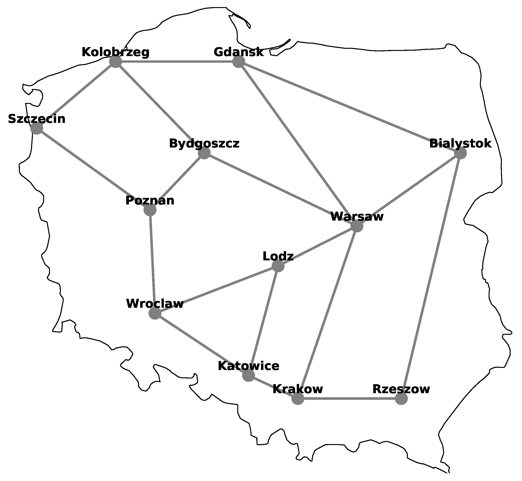
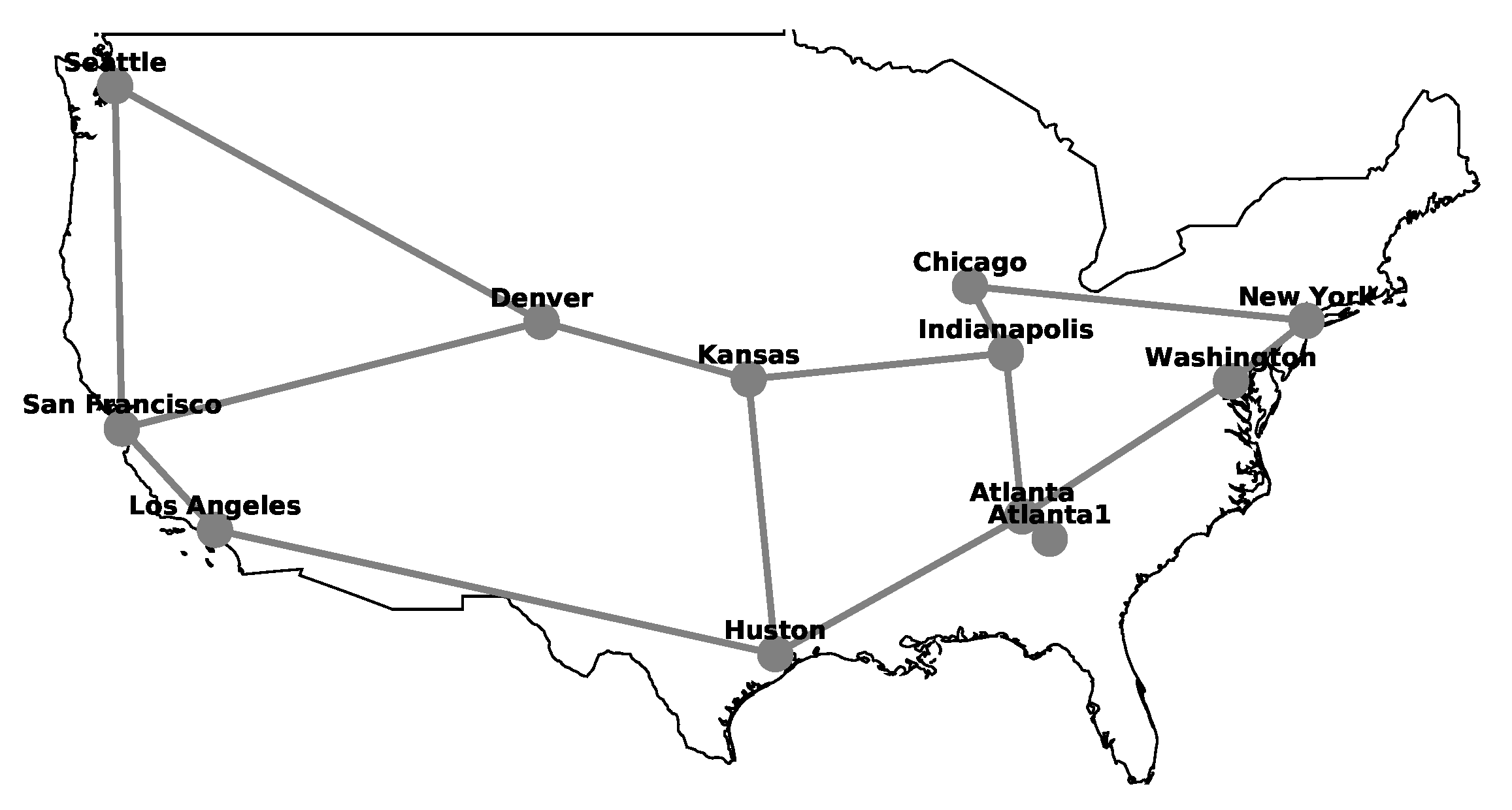
Computational results were obtained for three optical networks, Polish (Figure 3), American (Figure 4) and German (Figure 5), that have different characteristics. The networks correspond to actual optical networks stemming from specified countries and were taken from [19].

Table 1. Analyzed network parameters.

Network	# Nodes	# Link	# Demand
Polish	12	18	66
USA	12	15	66
German	17	26	136

and Figure 3, Figure 4 and Figure 5 provide the relevant parameters for both networks and their topologies.

The demands that were used in optimization of network cost, are given by demand matrix, which provides the values of traffic flow between selected nodes expressed in Gbps. An example demand matrix for the network from Figure 3 is presented in

Table 2. An example demands matrix.

	2	3	4	5	6	7	8	9	10	11	12
1	50	50	50	50	50	50	50	50	50	50	50
2		50	50	50	50	50	50	50	50	50	50
3			50	50	50	50	50	50	50	50	50
4				50	50	50	50	50	50	50	50
5					50	50	50	50	50	50	50
6						50	50	50	50	50	50
7							50	50	50	50	50
8								50	50	50	50
9									50	50	50
10										50	50
11											50

.

The calculations were carried out using a linear solver engine of CPLEX 12.8.0.0 on a 2.1 GHz Xeon E7-4830 v.3 processor with 256 GB RAM running under Linux Debian operating system. The average calculation time for Polish, American, and German networks was approximately equal to 56,000 s, 36,000 s, and 72,000 s, respectively.

The increase of traffic in an analyzed DWDM network was simulated by increasing the values of demand matrix elements (demands between initial and end nodes). It was assumed that all elements of the demand matrix were equal, i.e., set initially to 50 and then increased to 100, 300, and so on. The channels from C band were used first and L band channels were used only when C band ones were no longer available. For the sake of clarity, it is noted that on the abscissa axis the demand volume is measured using the value of a single demand matrix element, i.e., it is initially set to 100 and then increased to 300, 500, etc. until an integer solution is not feasible taking into account the available resources of the physical layer, i.e., a path for at least one of the demands cannot be provided.

Table 3. Sets description.

Set	Set Settings
$\mathcal{N}$	in Table 1
$\mathcal{E}$	in Table 1
$\mathcal{S}$	768 slots
$\mathcal{B}$	2 bands
$\mathcal{T}$	3 transponders
${\mathcal{S}}_b$	${\mathcal{S}}_1=\{1\dots 384\}$, ${\mathcal{S}}_2=\{385\dots 768\}$
${\mathcal{S}}_t$	${\mathcal{S}}_1=\{1\cdots 380\}\cup \{385\cdots 764\}$ ${\mathcal{S}}_2=\{1\cdots 378\}\cup \{385\cdots 762\}$ ${\mathcal{S}}_3=\{1\cdots 376\}\cup \{385\cdots 760\}$

describes in detail the sets and their settings and

Table 4. Modelling parameters.

Constant	Constant Settings
bitrate [Gbps]	$v\left(1\right)=100$, $v\left(2\right)=200$, $v\left(3\right)=400$
OSNR [dB]	$c\left(1\right)=$ 12, $c\left(2\right)=$ 15, $c\left(3\right)=$ 22
d(n,n’) [Gbps]	an example in Table 2
$\xi \left(b\right)$	$\xi \left(1\right)=1$, $\xi \left(2\right)=2$
$\xi (t,b)$	$\xi (1,1)=5$, $\xi (2,1)=7$, $\xi (3,1)=9$ $\xi (1,2)=6$, $\xi (2,2)=8.4$, $\xi (3,2)=11.8$
$\Delta \left(t\right)$ [GHz]	$\Delta \left(1\right)=$ 25, $\Delta \left(2\right)=50$, $\Delta \left(3\right)=75$,
$\nu \left(b\right)$ [THz]	$\nu \left(1\right)=193.8$, $\nu \left(2\right)=188.5$
$\mu \left(s\right)$ [dB/km]	$\mu \left(s\right)=0.046$ for $b=1$ and $\mu \left(s\right)=0.055$ for $b=2$
W [dB]	15
V [dB]	15
$P_0$ [W]	${10}^{-3}$

presents constant settings used during computational process.

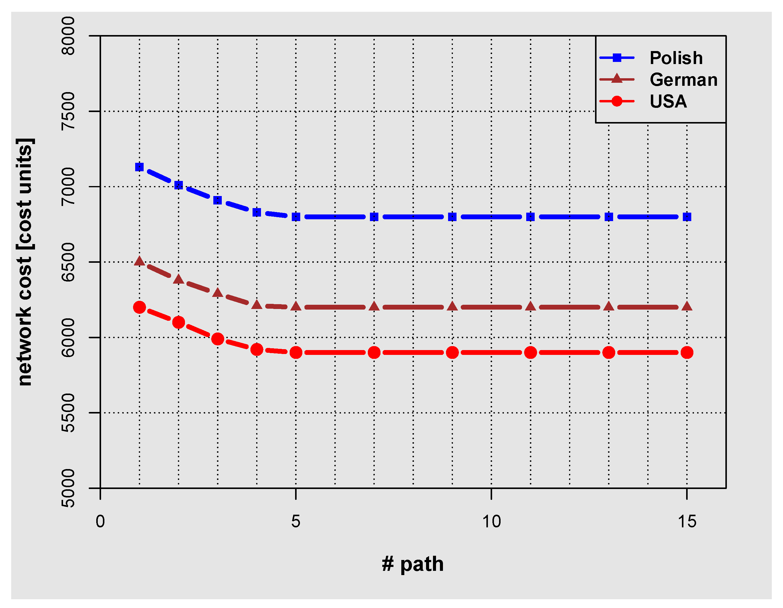
Figure 6 shows the dependence of network cost on the number of paths for Polish, American, and German networks calculated at the maximum value of the demand volume, which was $d=4500$, $d=3000$ and $d=2500$ for Polish, German, and American networks, respectively. The paths were selected using Yen’s K-shortest path algorithm [24].

In these calculations both C and L bands were used. The results from Figure 6 show that the network cost initially decreases with the increasing number of paths and then gradually levels off and settles to a constant value for the number of paths larger than 5. This indicates that increasing the number of available paths beyond 5 does not result in further significant reduction of the network cost while it may significantly increase the calculation time. Therefore the results shown in Figure 7, Figure 8, Figure 9, Figure 10, Figure 11 and Figure 12, were calculated with the number of paths set to 5.

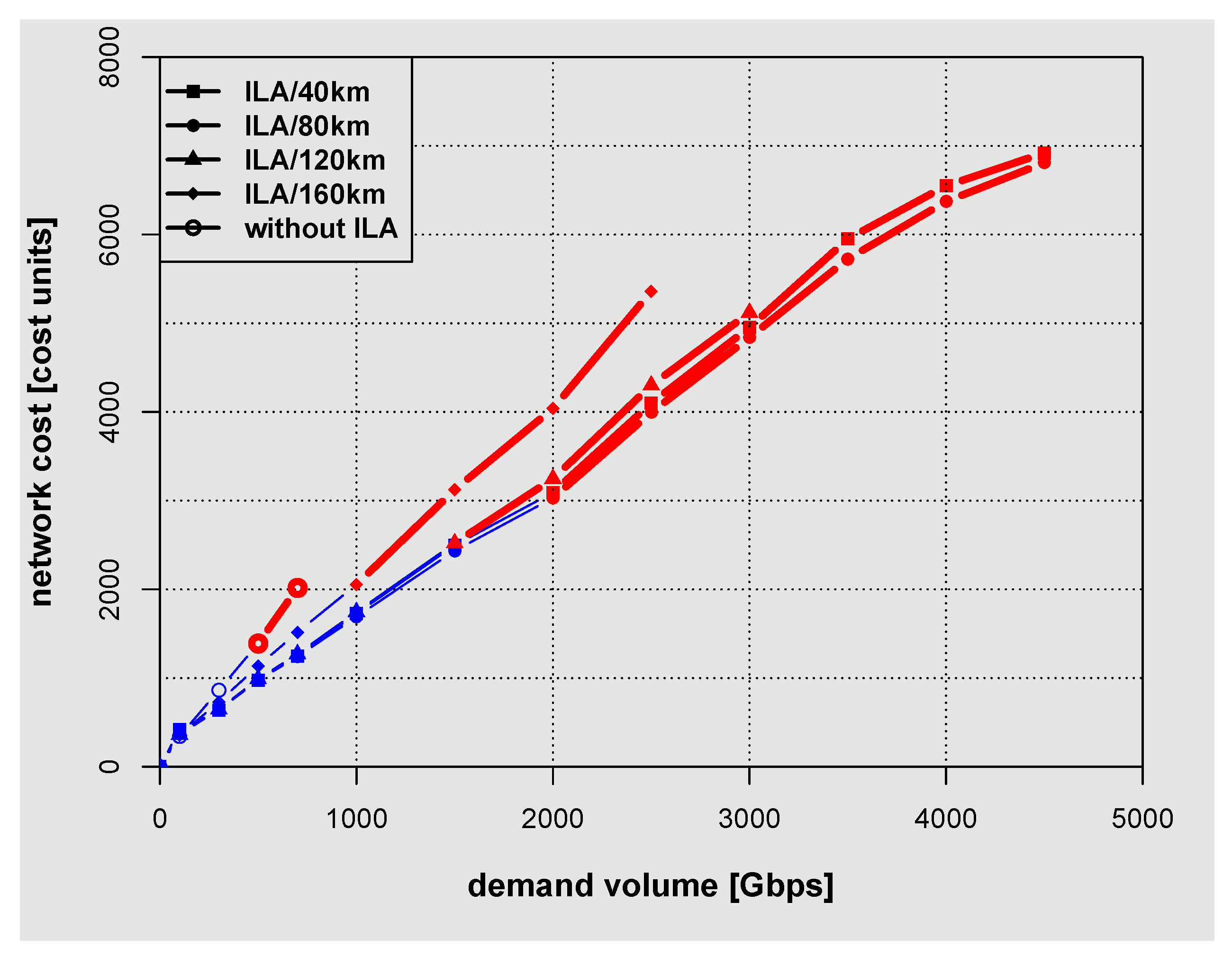
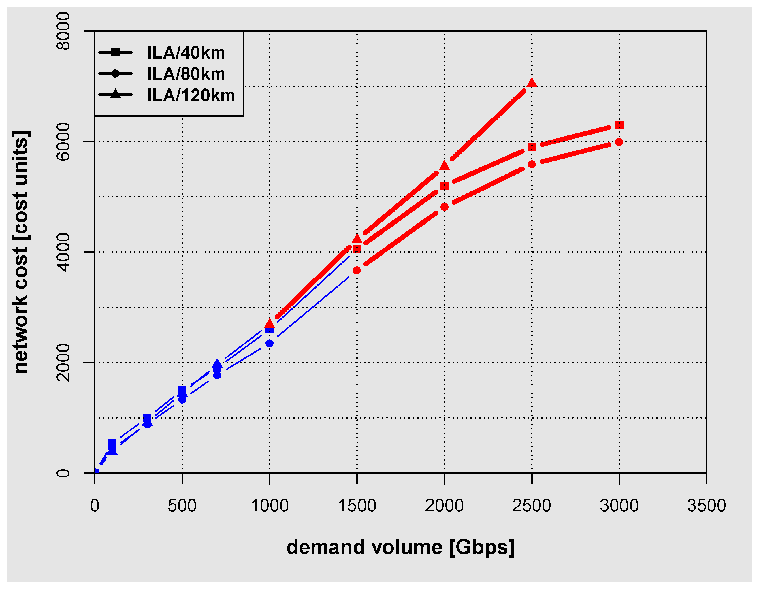
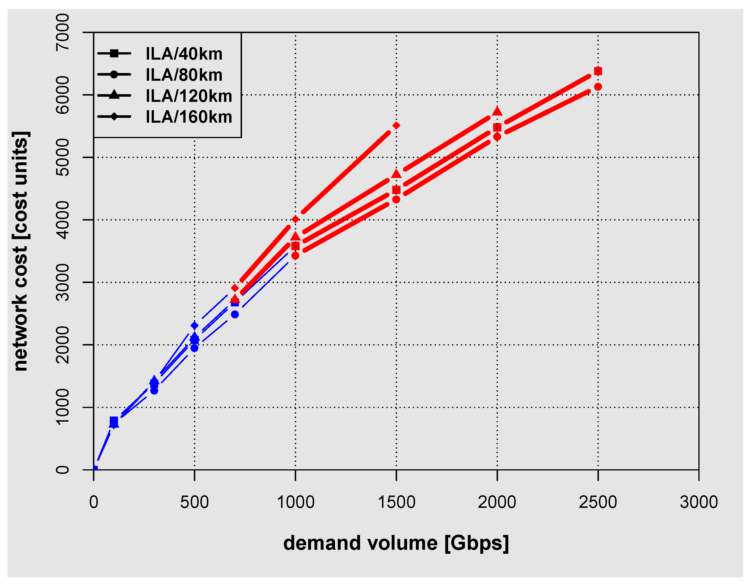
Figure 7, Figure 8 and Figure 9 present the dependence of network cost on the network capacity for Polish, American and German network. In Figure 7, Figure 8 and Figure 9 color coding is used to differentiate between lines representing the network costs obtained using C band only (blue thin line) and C + L band (red thick line). ILA were placed every 160 km, 120 km, 80 km and 40 km in each link of the network. The results shown in Figure 7, Figure 8 and Figure 9 indicate that using C and L band allowed more than doubling the amount of the allocated demand volume when compared with C band only. Interestingly, especially for cases with ILA spaced at 40 km and 80 km, the cost only doubles at most, when comparing the values for maximum allocated demand volume for C and L band (the end of red thick line) with C band only (the end of thin blue line). This is the case despite of the fact that nodal components (e.g., transponders and amplifiers) are by 20% more expensive for band L than for band C [25]. A closer inspection of the results shown in Figure 7, Figure 8 and Figure 9 reveals that the dependence of the network cost on the demand volume for Polish network is nearly linear for ILA spacing of 40 km and 80 km. However, for the German and American network the dependence of the network cost on the demand volume deviates more from a straight line. The ratio of the network cost to the demand volume for German network with ILA spacing of 80 km at demand volume of 1000 Gbps (maximum capacity for C band only) is equal approximately to 3.4 cost units/Gbps while for maximum capacity achievable using both C and L band it reduces to 2.4 cost units/Gbps whereas for the American network the ratio of the network cost to the demand volume reduces from 2.5 to 2 cost units/Gbps. For the Polish network however, the ratio of the network cost to the demand volume in both cases remains nearly constant and equal to 1.5 cost units/Gbps. Thus, in terms of the ratio of the network cost to the demand volume the largest benefits of using C and L band are obtained for American and German network. However, when one compares the maximum allocated demand volume for all three networks one can notice that the largest benefits from using C and L band are achieved for Polish and German network. For Polish and German network at ILA spacing of 80 km, the maximum allocated demand volume for C and L band is approximately 2.5 times that for C band only. For the American network only a twofold increase is observed. It is also noted that the results presented in Figure 7, Figure 8 and Figure 9 show that using ILAs too densely only increases costs without increasing the maximum allocated demand volume. In fact the best results for all three networks were obtained at the ILA spacing of 80 km, which agrees with engineering practice.

Potentially, an alternative solution to an implementation of ILAs is the use of Raman amplifiers either instead or in combination with ILAs. It is however, noted that a consistent delivery of Raman amplification over the entire L band up to 1625 nm, while the C band is in use, is not straightforward. ILAs on the other hand, for both the entire C and L band, are readily commercially available. Hence, here this latter route to improving a channel OSNR is studied.

The last point that needs to be explained is the lack of the results for large ILA spacing in the case of German and American network in (Figure 8 and Figure 9). This is due to a presence of long links. Specifically, in the case of American and German network results (Figure 8 and Figure 9) links with the length above 200 km for German network and most links for American network cannot be used without ILAs due to excessive signal attenuation and hence an unacceptably low OSNR. This in the context of the optimization procedures corresponds to an unfeasible solutions. Therefore, in order to make these links available for allocation it is necessary to place an ILA in the middle of a link to improve OSNR. Especially in the American network, which is a long-distance network, there is a need to use ILAs.

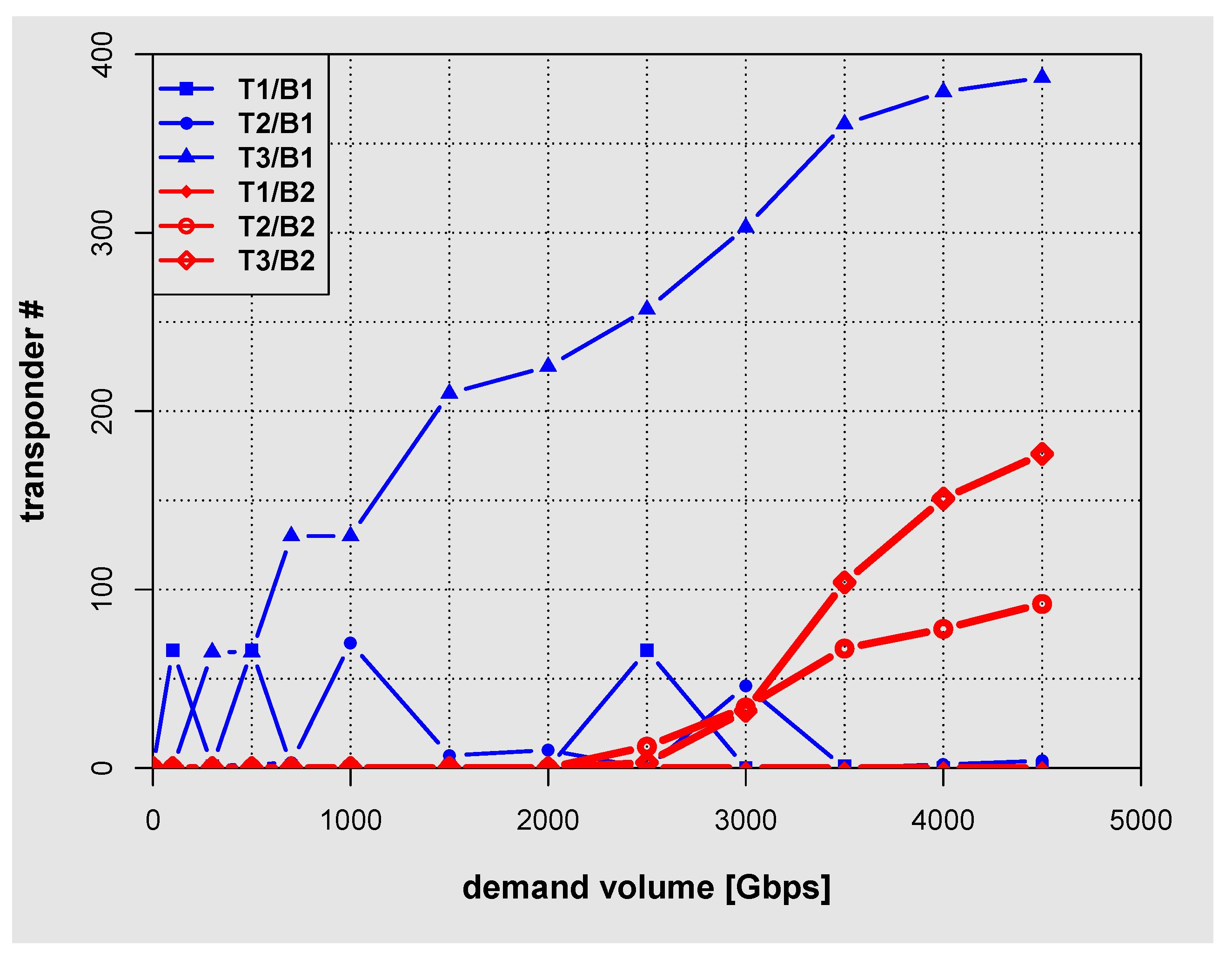
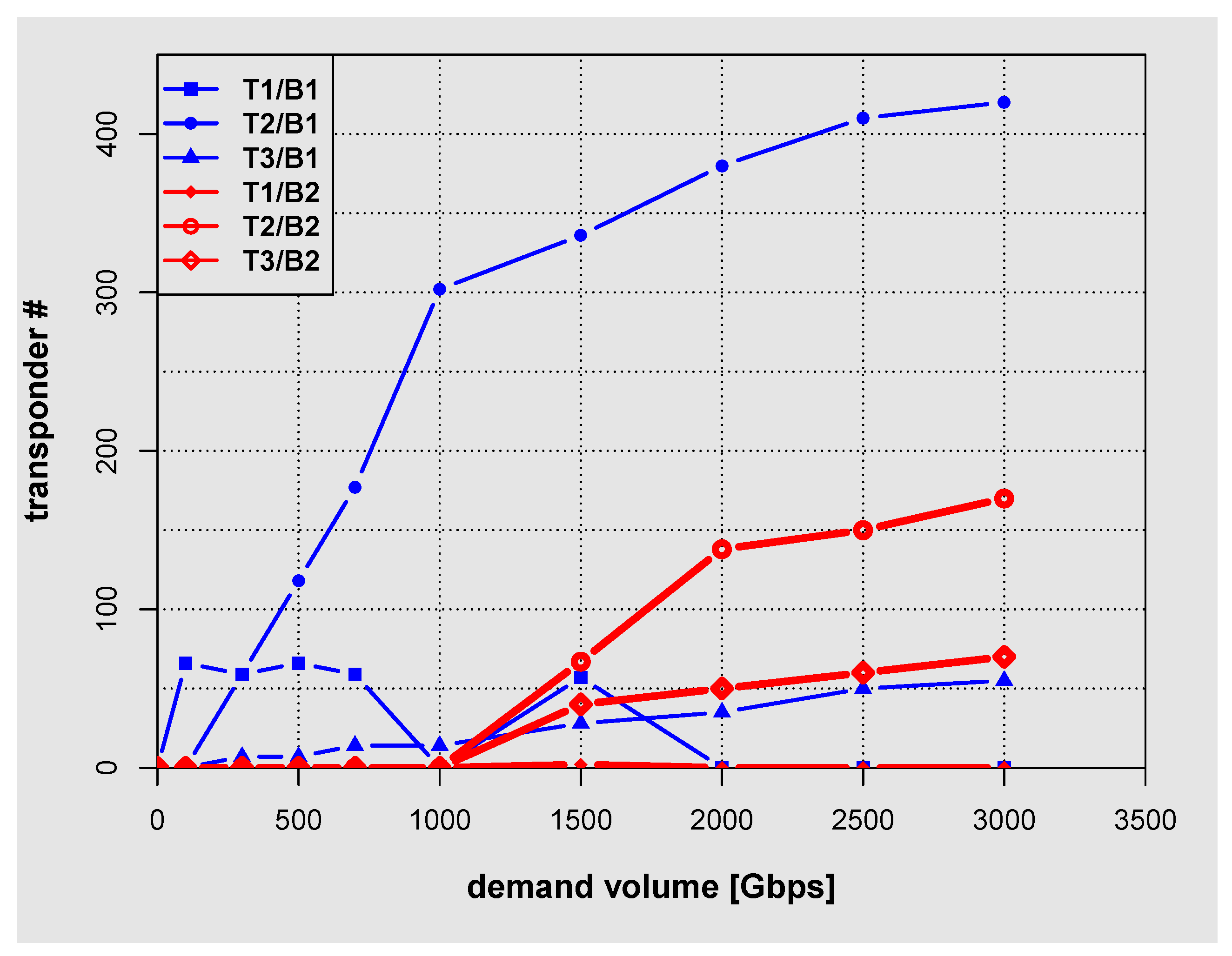
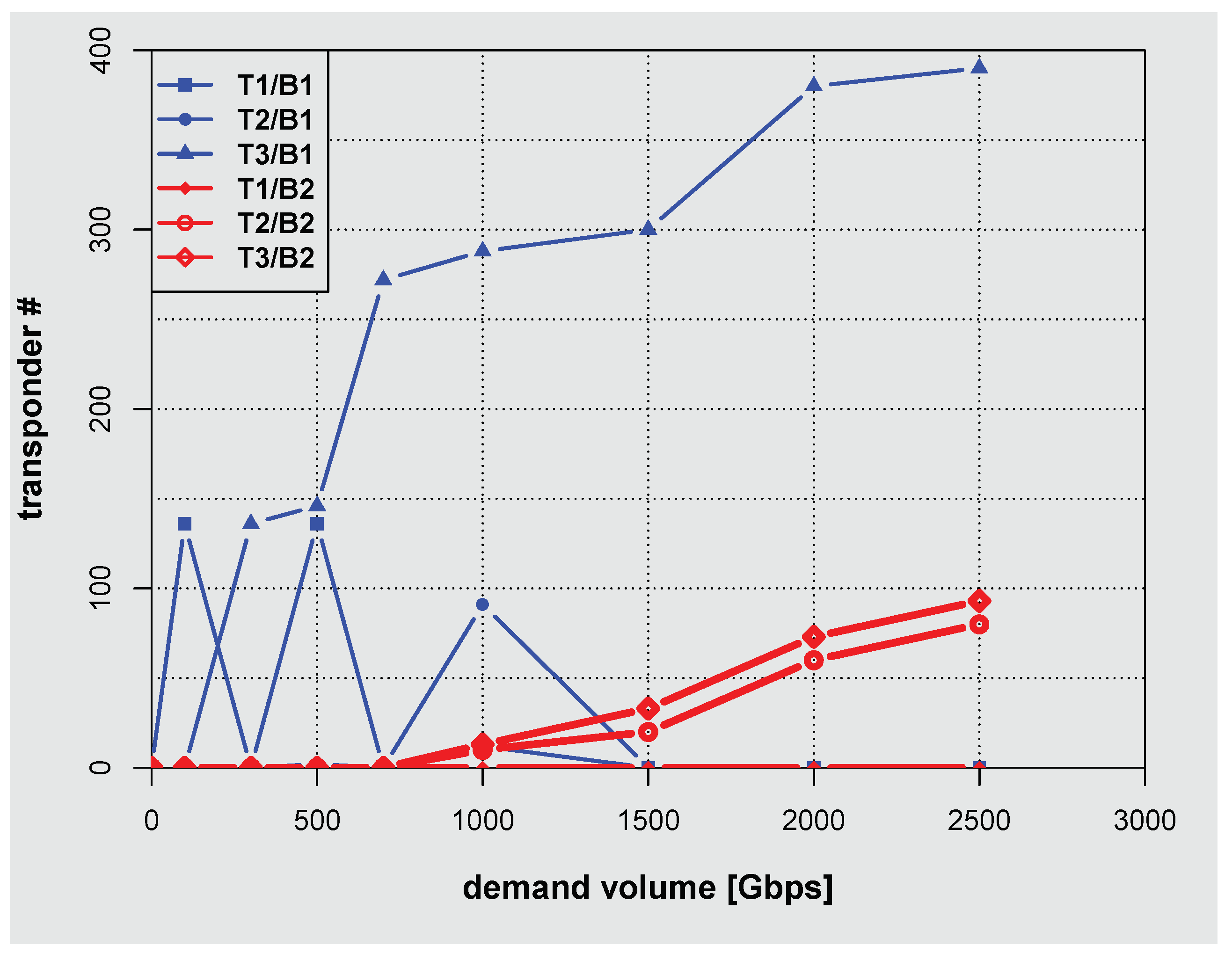
Results shown in Figure 10, Figure 11 and Figure 12 give the dependence of the number of transponders used on the demand volume and thus provide further insight into the optimal allocation of network resources with the increasing demand volume. The blue line corresponds to C band (B1) transponders while the red one to the L band (B2) transponders. Transponder bit rate for T1, T2, and T3 is given in Table 4 and is respectively 100, 200, and 400 Gbps. For the Polish and German networks the dependence of the number of transponders on the demand volume (Figure 10 and Figure 12) shows similar trends. In the case of Polish and German network at large values of the demand volume the dominant role is played by T3 transponder (for both C band and L band). In the case of American network (Figure 11) on the other hand, T2 transponder is mostly exploited at large values of the demand volume. Such behavior is related to the fact that in the American network, distances between nodes are large when compared with Polish and German networks and therefore transponders with higher throughput, characterized by larger required minimal OSNR value, cannot be used.

The up and down peaks visible in Figure 10, Figure 11 and Figure 12 result from the uniformity of the traffic matrices. The issue is clearly visible for 500 and 1000 Gps demands. The former demand is optimally satisfied using a pair of T1 and T3 transponders. On the other hand, the latter is optimally satisfied using two T3 and one T2 transponder. This behaviour is clearly depicted in Figure 10, Figure 11 and Figure 12.

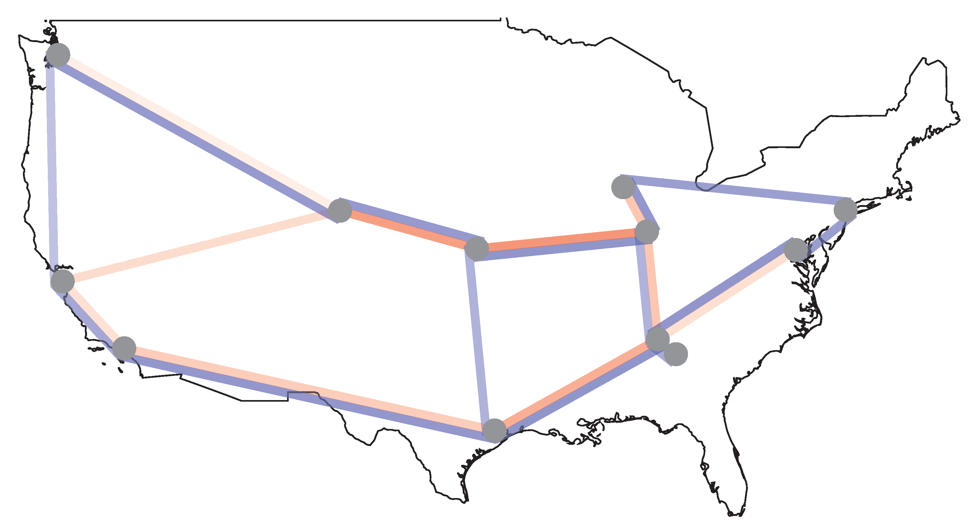
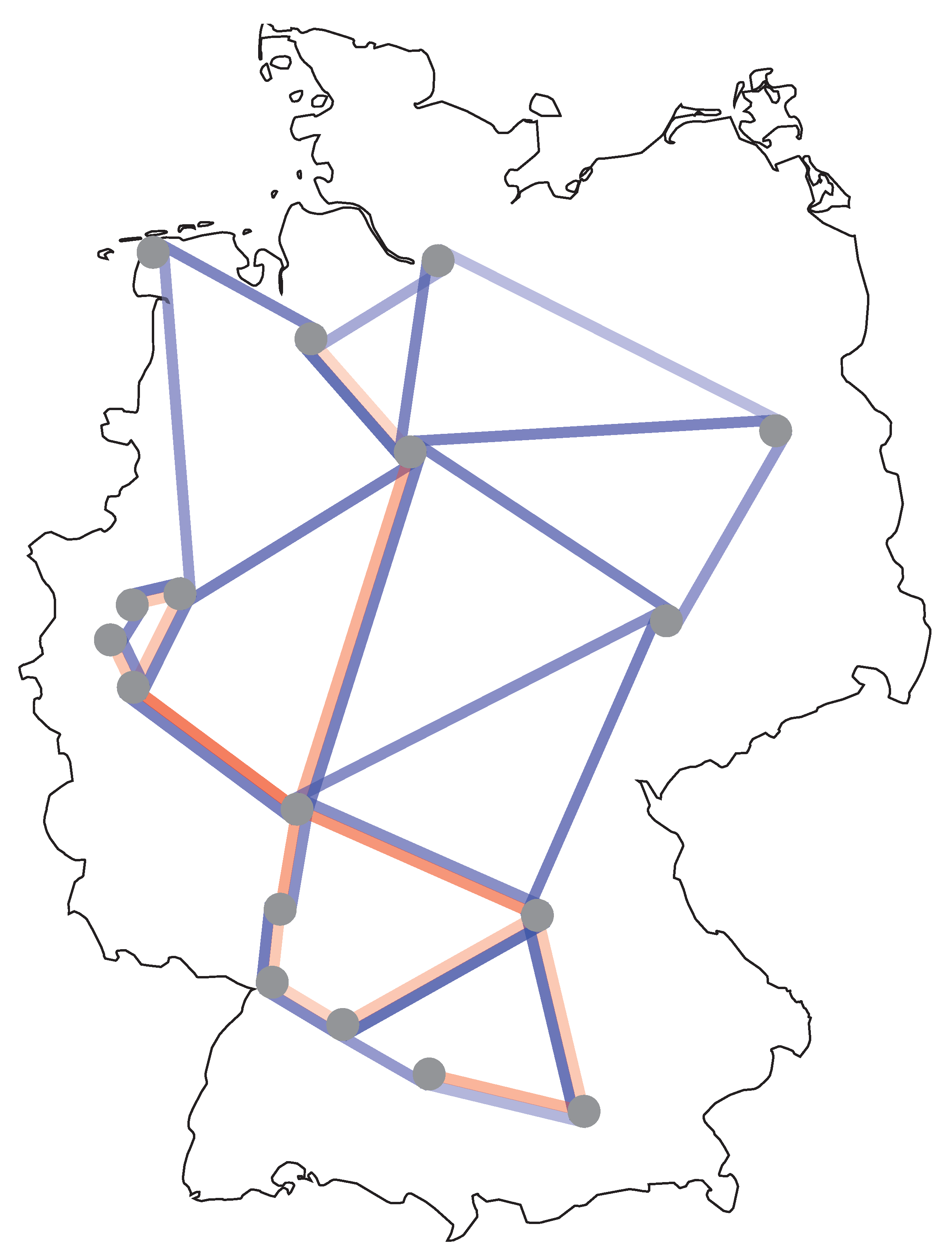
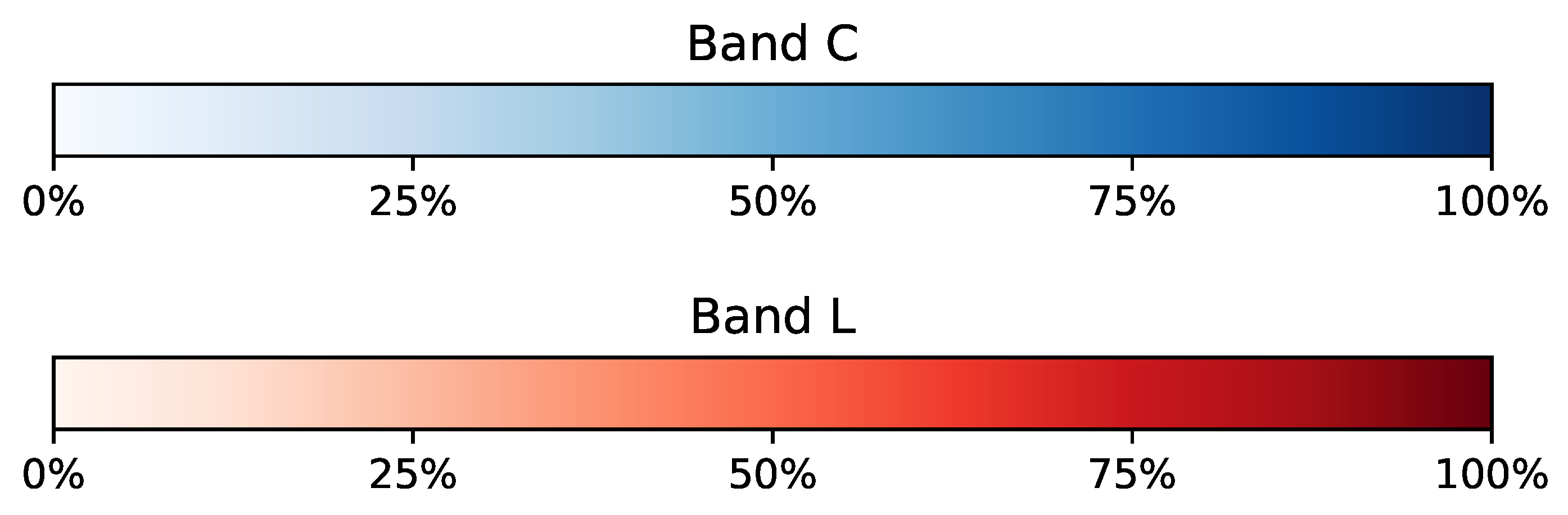
Finally, to gain more insight into the bandwidth usage for all links in Figure 13, Figure 14 and Figure 15 a diagram is plotted in a form of a map showing the percentage of the bandwidth used for each link. The legend for Figure 13, Figure 14 and Figure 15 is given in Figure 16. The red line intensity corresponds to the percentage use of the C-band while the red line to the L band, consistently with the colour coding used in the preceding figures. The results shown in Figure 13, Figure 14 and Figure 15 allow identifying the links that are used most and separate them from the links that are almost unused. For instance, there is a very limited use of the link between Denver and San Francisco in the case of American network (Figure 14) while the links between Denver and Kansas, and Kansas and Indianapolis are near the capacity limit. Also for the German and Polish networks the bandwidth usage in links is more evenly distributed than for the American network.

4. Conclusions

An optimization of an UW-WDM network that takes into account details of supported bands was performed. The study focuses particularly on the comparison of an UW-WDM network using both C and L band with a standard WDM network using C band only. The obtained results show that the UW-WDM network allows for nearly doubling the allocated demand volume when compared with the standard WDM network operating within the C band only.

The results obtained show also that there is a significant qualitative difference in the operation of the American network when compared with the Polish and German networks. First of all the distribution of network traffic within the Polish and German networks is more uniform than in the American network. Secondly, the Polish and German networks make much more extensive use of high bit rate transponders when compared with the American network. The reason for these differences is attributed to large inter-nodal distances that characterize exclusively the American network.