
Worldwide Evaluation of CAMS-EGG4 CO2 Data Re-Analysis at the Surface Level


1
Helmholtz-Zentrum Hereon, Institute of Coastal Environmental Chemistry, Max-Planck-Str. 1, 21502 Geesthacht, Germany
2
Max-Planck Institute for Biogeochemistry, 07747 Jena, Germany
3
CESAM & Department of Environment and Planning, University of Aveiro, 3810-193 Aveiro, Portugal
*
Author to whom correspondence should be addressed.
Toxics 2022, 10(6), 331; https://doi.org/10.3390/toxics10060331
Submission received: 23 May 2022
/
Revised: 14 June 2022
/
Accepted: 14 June 2022
/
Published: 17 June 2022
(This article belongs to the Special Issue Modelling & Impacts Assessments of Air Quality)
Abstract
:This study systematically examines the global uncertainties and biases in the carbon dioxide (CO2) mixing ratio provided by the Copernicus Atmosphere Monitoring Service (CAMS). The global greenhouse gas re-analysis (EGG4) data product from the European Centre for Medium-Range Weather Forecasts (ECMWF) was evaluated against ground-based in situ measurements from more than 160 of stations across the world. The evaluation shows that CO2 re-analysis can capture the general features in the tracer distributions, including the CO2 seasonal cycle and its strength at different latitudes, as well as the global CO2 trend. The emissions and natural fluxes of CO2 at the surface are evaluated on a wide range of scales, from diurnal to interannual. The results highlight re-analysis compliance, reproducing biogenic fluxes as well the observed CO2 patterns in remote environments. CAMS consistently reproduces observations at marine and remote regions with low CO2 fluxes and smooth variability. However, the model’s weaknesses were observed in continental areas, regions with complex sources, transport circulations and large CO2 fluxes. A strong variation in the accuracy and bias are displayed among those stations with different flux profiles, with the largest uncertainties in the continental regions with high CO2 anthropogenic fluxes. Displaying biased estimation and root-mean-square error (RMSE) ranging from values below one ppmv up to 70 ppmv, the results reveal a poor response from re-analysis to high CO2 mixing ratio, showing larger uncertainty of the product in the boundaries where the CAMS system misses solving sharp flux variability. The mismatch at regions with high fluxes of anthropogenic emission indicate large uncertainties in inventories and constrained physical parameterizations in the CO2 at boundary conditions. The current study provides a broad uncertainty assessment for the CAMS CO2 product worldwide, suggesting deficiencies and methods that can be used in the future to overcome failures and uncertainties in regional CO2 mixing ratio and flux estimates.
1. Introduction
More than ever, carbon dioxide (CO2) monitoring is at the front line of climate change mitigation. Taking the lead in climate transition and emission control has become imperative. Nonetheless, the capability of monitoring atmospheric CO2 by combining numerical models, in situ and remote sensing observations has rapidly evolved to improve our understanding of CO2 fluxes, sources and sinks [1,2].
The integration of earth observation data may become a critical tool in supporting policies aimed at reducing CO2 emissions, a key anthropogenic driver of climate change [2,3]. Human activities are directly responsible for most of the CO2 emissions, particularly due to the use of fossil fuel, with emissions particularly high in urban areas. With a lifetime of hundreds of years and well-known sources, CO2 essentially disperse after being emitted, and reliable data-product of such atmospheric trace gas can be critical in studies of air pollution dispersion and source apportionment of many atmospheric trace gases [4,5]. In addition, it can potentially provide a second option for evaluating national inventory [6].
Monitoring global CO2 emissions is highly desirable. To support and foster such a system initiative, the ECMWF Integrated Forecasting System (IFS) provides global gridded estimates of the atmospheric CO2 mixing ratios. In the global greenhouse gas re-analysis dataset (EGG4), the CO2 fluxes from natural and anthropogenic sources are modeled, even making use of a coarse time-resolution inventory (monthly). This provides CO2 fluxes in the atmosphere in a wide range of scales, from diurnal to inter-annual.
The Greenhouse Gas re-analysis dataset from Copernicus Atmosphere Monitoring Service, CAMS-EGG4, makes intense use of data assimilation. It combines high-resolution global models together with in situ CO2 concentration networks across the world, as well as satellite data. This results in a globally complete and consistent dataset using a model of the atmosphere based on the laws of physics and chemistry.
To make CAMS-EGG4 data more reliable in understanding sources, sinks and the transport of atmospheric CO2 from the surface into the troposphere around the globe, the reliability of this data product should be evaluated based on fiducial observation measurement comparison. Quantifying the quality of such data products by decomposing the inherent uncertainty components is a challenging and key component in product reliability and its use. The overall objective in validating and evaluating uncertainties of earth observation data products, such as those provided by CAMS, is to explicitly answer the question: How good is the evaluated dataset?
Hence, the study aims to explore the potential of CAMS to monitor and analyze CO2 concentrations at global scales. We attempt to compare the CAMS CO2 data at surface level with high accurate in situ surface data.
As a contribution to the evaluation of CAMS-EGG4 CO2 re-analysis data, the atmospheric concentration of CO2 provided by CAMS were compared with observational data gathered by monitoring ground stations. The reference data used to evaluate the performance of CO2 data from the CAMS re-analysis at surface level consist of high-resolution in situ observations obtained from extensive CO2 measurement programs, such as Global Atmosphere Watch (GAW), Amazon Tall Tower Observatory (ATTO) and the Global Monitoring Laboratory of the National Oceanic and Atmospheric Administration (NOAA).
A comprehensive validation report for the global CAMS CO2 re-analysis is reported by Ramonet et al. [7], based on airborne observation and 23 background stations worldwide. The aforementioned authors reported an increasing near-surface bias and regional uncertainties associated with vegetation model features representing biogenic fluxes. However, further evaluation of CAMS re-analysis seeking the main sources of errors is still needed to understand its product compliance and misfit. In addition, such a study can bring insights into the CO2 fluxes parametrization considered in the CAMS model.
The product strength and concerns were enhanced by understanding the differences among observations and the product and the spatial differences. In comprehensive statistics comparing measurement data from hundreds of stations, we assess the compliance of the re-analyses of CO2 on a global basis. Furthermore, we discuss the re-analyses and observation mismatches, exploiting the model constraints reproducing concentration at boundary regions and anthropogenic fluxes.
2. Datasets and Methods
2.1. Datasets
To evaluate the compliance of the CAMS CO2 product, we selected 160 worldwide sites monitoring this trace gas. The following subsections briefly describe the datasets considered in this study.
2.1.1. CAMS-EGG4
The Copernicus Atmosphere Monitoring Service (CAMS) implemented by the European Centre for Medium-Range Weather Forecasts (ECMWF) is one of the most advanced global atmospheric models simulating the state of the atmosphere with accuracy similar to what is theoretically possible using a 4D-Var method [8,9].
CAMS provides trace gas products such as greenhouse gases for downstream applications in early warning systems, environmental monitoring, health services and climate research [10].
Known as the Integrated Forecasting System, it is a component of the Copernicus European Earth observation program. It was originally developed through a series of Monitoring Atmospheric Composition and Climate (MACC) research projects (MACC I-II-III) that provide near-real-time and re-analysis systems with modelling and data assimilation of trace gas mixing ratios and aerosol concentrations. In this study, we used CO2 from CAMS global greenhouse gas re-analysis (EGG4) products obtained from the Copernicus platform. The CAMS-EGG4 CO2 product evaluated refers to re-analysis model level products downloaded in July 2021/September 2021 at the CAMS catalogue [11]. The re-analysis CO2 CAMS-EGG4 data are available at three-hour intervals (starting at 00:00 UTC) and on a regular latitude–longitude grid of 0.75° × 0.75°. This study used products retrieved at the model levels 60, 59, 58, 57, 56, 55, 54, 53 (10 m, 34 m, 71.89 m, 124.48 m, 195.85 m, 288.57 m, 404.74 m and 546.11 m) geometric altitude described at https://confluence.ecmwf.int/display/UDOC/L60+model+level+definitions (last access on 1 May 2022). As a global re-analysis grid, it can be interpolated to the desired location, and its accuracy is based on the error characteristics of the assimilated data.
The CAMS makes intense use of satellite assimilation; it also assimilates atmospheric observations from aircraft networks [12] and radiosondes [13]. CAMS-EGG4, currently covering the period 2003–2020, uses 4DVar data assimilation in CY47R1 of ECMWF’s Integrated Forecast System (IFS). This system is continuously improving through the addition of new features and new model versions.
CAMS-EGG4 assimilates surface CO2 fluxes from the terrestrial biosphere directly into the IFS using the CTESSEL carbon module [14]. Other sources and sinks of CO2 are prescribed from different inventory sources and datasets. The CO2 fluxes are not directly updated by the observations assimilated, but an online flux correction scheme is applied to correct bias. Such correction is performed by comparing the modelled biogenic fluxes with a climatology of optimized fluxes. CAMS meteorological initial conditions come from the ECMWF operational analyses. The specific EGG4 model configuration is documented in the listed papers below:
- Bias correction for CO2 ecosystem fluxes based on the Biogenic Flux Adjustment Scheme is documented by Agustí-Panareda et al. [17];
2.1.2. Ground-Based Observation
To evaluate the performance of CO2 provided by the CAMS model (EGG4), we used “ground truth” data from ground stations. We used continuous CO2 observations from more than 160 in situ monitoring stations established in worldwide monitoring programs.
Monitoring towers for ground-based measurements facilitate the measurement of greenhouses gases. We used data from the following: the Global Atmosphere Watch (GAW) program of the World Meteorological Organization (WMO); the National Oceanic and Atmospheric Administration (NOAA) in the United States, a scientific and regulatory agency; and the Amazon Tall Tower Observatory (ATTO). In addition to Tall Tower, seven other tower stations sampling at different altitudes were used in this study, providing observation data up to 457 m height (agl). The ground-based monitoring system provides the physical and chemical references of CO2 concentration to evaluate global earth observation data products. The GAW, NOAA and ATTO observing projects provide datasets and services to decision-makers and the public, as well as for scientific evaluation and forewarning of changes in the air composition that may have adverse effects on the environment [21]. The ground stations can provide handy insights in evaluating earth observation data products as they are spread worldwide and provide accurate high-resolution data (0.1 ppmv).
To estimate the accuracy of global CO2 re-analysis from CAMS, we selected the ground surface stations at different locations and altitudes. The selected sites are appropriate because they cover a long period of CAMS CO2 data availability, if not the entire period. The location of those stations (Figure 1), and the entire site description, are shown in the hypergraph at https://rpubs.com/danilocustodio/874276.
2.2. Methods
For comparability with the re-analysis CO2 product, the observation data were averaged over three-hour periods. The observation data from ground stations at a 3 h resolution were considered valid only if they had values for at least 75% of the time.
The re-analysis (EGG4) products were downloaded at the regular latitude–longitude grid of 0.75° × 0.75° and then interpolated to observation data colocation. Despite the different spatial resolutions, the mean value of upper gridded earth observation products can be used to match up with ground monitoring sites [25,26].
Based on kernel-smoothing interpolation, the CO2 data products used in the comparison were interposed linearly in latitude, longitude and polynomially (second order) in atmospheric pressure to the same height as the measurement data.
After spatiotemporal collocation of CAMS and observation could be spatiotemporally aggregated and pairwise datasets were compared. The CAMS product and observations are compared, analyzed and discussed at the observation correspondent position. In this study, the temporal and spatial comparisons were performed for as long as it was conceivable and as broadly as possible, depending on the observation data availability.
After retrieving the CO2 product from the respective observation coordinates, temporal collocated pairwise datasets could be compared based on five metrics: The first metric is the mean difference between product values and observations, defined as root-mean-square error (RMSE) which shows the differences between product values and observation at different station sites. The RMSE is defined as (Equation (1)):
where N is the total number of observations, and Xproduct and Xobservation are the CO2 mixing ratio for the product and observation, respectively. The second metric is relative differences (% difference) defined as the percentile difference of the product compared to the reference (Equation (2)).
The third metric is mean bias (MB), or mean bias error (Equation (3)), which display the average bias in the CAMS-EGG4.
The fourth adopted metric is the linear regression deployed to evaluate the conditional probability distribution of the product’s prediction (conditional quantile). Last but not least, kernelized temporal pattern is deployed to find and evaluate the temporal alignments among product and observation.
2.3. Representative and Spatial Scale Issues
Despite the different spatial resolutions, the mean value of models in an amplified grid cell is usually used to match up with ground monitoring sites [25,26].
However, it is worth highlighting two important issues when performing comparisons between gridded data such as those from CAMS, which have a large spatial coverage, and point-like ground-based observations: (i) a ground observing station might not be representative of the entire concentration over a grid cell, particularly in the case of a grid with intense sources, or in the vicinity of the sources; and (ii) the pixel-mean elevation of the surface (in gridded data) and the actual station elevation are not necessarily representative of the product layer.
These issues introduce errors and affect all comparative studies of this kind [27,28,29,30,31,32]. To mitigate this, the present study includes the comparison of aggregated factors of temporal pattern. In addition, we apply scale-height correction by interpolating the product dataset available at different layers to the height of the “ground truth” reference data.
3. Results and Discussion
In this section, we present the main results from the evaluation of the carbon dioxide re-analysis data product provided by CAMS. To evaluate the compliance of CAMS-EGG4 compared to the observation, we apply mean bias, root-mean-square error (RMSE), relative differences, regression analysis and temporal patterns. Beyond the qualitative agreement and disagreement among the datasets, we assess the compliance strength of the CO2 product. Based on the five used metrics, we investigate the product’s misfit on the bias, response to temporal variation and uncertainties.
3.1. Overall Performance of Re-Analysis
The root-mean-square error (RMSE), average absolute errors in percentage, mean bias and slope regression between CAMS-EGG4 and observations are extracted from the entire available data and are presented at https://rpubs.com/danilocustodio/874273 (Figure 2). This hypergraph shows the data comparison between CAMS-EGG4 and observations at different sites considered in this study. The overall RMSE (Cobservation, CCAMS-EGG4) was 17.59 ppmv, the mean bias (Cobservation, CCAMS-EGG4) was 7.46 ppmv and the slope of the linear regression (Cobservation, CCAMS-EGG4) was 1.018.
The evaluation of the global performance of CO2 re-analysis from CAMS reveals a lower RMSE and a lower percentage of error at stations in remote environments, such as at the North and South Poles, in the Pacific, Atlantic and the Indian Oceans. On the other hand, higher disagreement among the compared datasets was mainly at stations in continental regions.
The evaluated CO2 products were low biased and statistically similar to measurements (in 95% confidence interval in the mean) at the remote end stations, such as at the South Pole, King George Island, Samoa, Cape Verde, Azores, Barrow, Alert, Amsterdam Island, Macquarie Island, Ascension, Crozet, Mawson and Casey. At the aforementioned stations (georeferenced in https://rpubs.com/danilocustodio/874273), there is a difference of less than 0.5% between the CAMS data and the observations. On the other hand, differences rise above 6% at stations such as Amazon Tall Tower, Fundata, Monte Cimone, Bukit Kototabang, Pha Din, Mt. Dodaira, Suita, Kisai, Anmyeom-do and King’s Park. Notable differences were also observed at Farafra and Cairo stations; however, those stations have recently raised questions regarding their data quality control.
The minimum deviation of the CAMS data, less than 1.4 ppmv, was observed at Storhofdi (Iceland), Ascension Island (South Atlantic), Antarctic Station and Macquarie Island (Pacific Ocean), while the maximum deviation, above 50 ppmv, was observed at Danum Valley and Bukit Kotatabang (South Asia), Mt. Dodaria and Kisai (Japan). As shown in Figure 2, the CAMS-EGG4 data are in good agreement with CO2 observed at surface level in regions far from CO2 sources, indicated by a well-mixed ratio of this gas in the atmosphere. However, the CAMS product shows concentration dependence displaying significant bias at high CO2 concentrations (Figure 3). The average deviation between the CAMS data and observation is 2.4% (12.8 ± 15.5 ppmv). The reason CAMS overestimates CO2 in continental regions, as displayed in Figure 2, is likely related to different factors such as source consideration and transport modelling parametrization in the CAMS model. In addition, the Tall Tower data show that the differences are not vertically homogeneous; CAMS re-analysis data exhibit a strong gradient with improved performance at higher altitudes (Table S1, https://rpubs.com/danilocustodio/874273). The reasons for this could be attributed to the carbon sources and sinks at the near surface combined with atmospheric mixing, determining the spatial distribution and temporal variation of CO2 in the lower troposphere. The higher stratification of the atmospheric boundary can lead to large CO2 gradients that are more difficult for the re-analyses to accurately capture.
3.2. Compliance and Misfit
Figure 3 shows the conditional quantile plots where the re-analysis CO2 data are evaluated against the ground-based observations. The aforementioned figure illustrates the regression between re-analysis data derived from CAMS and observation at surface level for the worldwide stations described in Figure 1. The results indicate agreement among the dataset at more than 90% of the distribution. However, pronounced differences are displayed on the edges of the distribution when CAMS mainly overestimates CO2 concentrations and constrains bias above the 10/90th percentile. The CAMS data shows an increasing bias, up to 60 ppmv, at regions where potential nearby pollution sources are present. The misfit at the continental stations is probably due to the influence of CO2 fluxes close to the station, which are not spatially well resolved by the CAMS model, as is discussed in the next section.
As displayed at Barrow Station, CAMS could respond reasonably well at remote regions with low concentration variation in space. Displaying compliance in the 25/75th conditional quantile, the CAMS product could be an important reliable data source in remote ends or regions with a homogeneous distribution of CO2 mixing ratio.
As shown in Figure 4 for two specimen stations, the re-analysis matches the observation quite closely. However, the re-analysis shows a positive bias before 2013 and an increasing negative bias after that year. This bias and its signal break in 2013 are more easily detectable at stations in the southern hemisphere, such as at the South Pole, thanks to the weakness of the seasonal cycle. Still, it is present at other latitudes as is faintly displayed at Barrow. The bias inversion in 2012/2013 corresponds to the end of data assimilation from the SCIAMACHY instrument in 2012 and the start of assimilation of IASI-B data in 2013 [7].
The CAMS system reproduces the CO2 atmospheric background trend and seasonality fairly well. The performance of the re-analysis is compliant with the observed atmospheric CO2 trend in a 99% significance interval. The seasonal variability differs significantly from site to site. It is more pronounced in the northern hemisphere, which is explained by different biogenic fluxes, depending on the type of ecosystem (e.g., crops or forest areas) in the station footprint. The vegetation model in CAMS represents this well (Figure 5).
We find that the temporal profiles of CO2 from CAMS re-analysis can agree exceptionally well with the CO2 temporal variability of ground-based observation at regions with low anthropogenic flux. The CAMS analysis appears to capture the biogenic fluxes in oceanic and terrestrial regions. For instance, a maximum diurnal variation of 1 ppmv was observed for oceans and terrestrial regions with a well-mixed CO2 ratio (background regions), with maxima at noon, when observed. Chen et al. [33] reported that the biogenic CO2 surface fluxes are provided by an online biosphere model in the IFS system. In addition, biases are corrected in real time throughout the forecast.
3.3. Main Sources of Error
Emissions and dynamics explain most of the differences in observation-data products comparisons [34].
Second Hedelius et al. [34] about 25% of the differences among CO2 data product and observation can be associated with the proximity of anthropogenic sources of CO2 combined with the basin topography that can lead to the trapping of polluted air enhancing CO2 concentration gradient within the basin. Such events are not solved by atmospheric models. This error is mainly associated with errors in the estimation of mixed layer height, leading to significant errors in retrieved fluxes. Kort et al. [35] and Newman et al. [36] attributed this phenomenon almost entirely to anthropogenic emissions.
As reported by Lian et al. [37] sources of misfits include uncertainties in the atmospheric transport, in atmospheric CO2 conditions that are used at the boundaries of the model, in the natural CO2 fluxes within the modeling domain, and in the spatial and temporal resolution and distribution of the inventories used in the model.
Uncertainties in modeling the atmospheric transport of CO2 are exacerbated in urban areas due to building obstacles (roughness) that generate specific mixing processes and modify the wind speed and direction [37]. This also occurs in misestimation of urban biogenic fluxes [38].
The uncertainties in the assumed temporal and spatial emission variations induce a critical source of error poorly constrained by the inversions due to the lack of boundary data [39,40]. The CAMS anthropogenic emission inventory’s spatial and temporal allocation has a monthly spatial grid resolution of 0.1° x 0.1°. The inventory accounts for emissions from different sectors, such as the transportation, residential and energy sectors, as well as biogenic fluxes [41]. Potential sources of CO2 not far from a station can cause variations in atmospheric CO2 that are not captured by the model grid cell, which are resolved in kilometric scale.
Uncertainties in atmospheric transport of CO2 are exacerbated in areas near sources where mixing processes and variation in wind speed and direction can significantly take place.
The results presented in this article show systematic biases in the re-analyses at mixing ratios above 420 ppmv. Further examination shows that most CAMS biases and high RMSE are located in regions with intense anthropogenic sources, especially in Asia. To analyze the errors constrained by uncertainty in anthropogenic fluxes, we evaluated the diurnal pattern of observation and re-analysis at the different stations, such as Kisai, Mt. Dodaria, Mikawa-Ichimomiyia and Suita in Japan, as well at stations in South Asia and Europe, where the re-analysis displayed high miss estimation. Those stations have the highest CO2 mixing ratios and are within or in the proximity of urban areas, potentially providing strong signatures of anthropogenic emissions.
Figure 6 shows the diurnal variation of CO2 at selected sites with high RMSE. For instance, the observation shows a flux of CO2 during the day. The most common pattern of diurnal variation displays a decrease of CO2 mixing ratio at noon. This could be linked to biogenic uptake and the sensible heat emissions at the surface that enhance vertical mixing in urban environments with the increase in depth of the boundary layer (Lian et al., 2021).
Regions with high CO2 mixing ratio, such as urban and suburban areas, have green spaces and are surrounded by rural areas that can actively take up CO2 in the daytime during the growing season.
Parametrization of CO2 fluxes misestimating the daytime biogenic respiration is a significant source of modeling error during the growing season outside the city or in regions with significant vegetation cover. The CO2 concentration is also influenced by remote emissions and large-scale biogenic fluxes in incoming air masses when the wind blows from green areas into urban environments [42].
The re-analysis shows a diurnal cycle amplitude quite different from the corresponding observation at stations such as Mt. Dodoira, Kisai, Mikawa-Ichinomiya and Suita. The most striking error is the concentration amplitude throughout the day when the observation shows a variation in CO2, while the re-analysis misestimates such fluxes.
The impact of anthropogenic fluxes in continental conditions of high CO2 concentration, where the re-analysis performance is relatively small, would be associated with the signature of the anthropogenic emissions constrained in the IFS model, which are not observed in reality.
Since CAMS assimilates only infrequent remote sensing XCO2 measurements from the polar-orbiting satellite [32], the observations are likely insufficient to correct this bias. In addition, part of the bias may be inherited from biases in the satellite retrievals and their boundary limitation [16,43].
The good representation of annual cycle and the decrease in flux emissions during the daytime and an increase during the nighttime, in almost all stations with well-mixed CO2 ratio, is a strong indication that the seasonal and diurnal profile of the biogenic CO2 emissions is well represented in the IFS model in remote regions. On the other hand, the amplitude in the diurnal profile at regions with high CO2 mixing ratios could indicate an erroneous CO2 emission/sink in the CAMS inventory, and a flux parametrization, as an improved diurnal pattern, is needed.
Errors in atmospheric transport also contribute to the re-analysis data misfit. The overestimation of the daytime CO2 mixing ratio, not only at the urban sites, but also at rural stations, is evidence of the flux parametrization deficiency. This mismatched pattern in the fluxes can embed a difference in the re-analysis of up to 80 ppmv that can explain most of the RMSE from the CO2 re-analysis. The IFS system may overcome these errors related to CO2 fluxes in boundary conditions by improving anthropogenic fluxes parametrization in urban/suburban/rural regions, as well as improving biogenic fluxes parametrization in those regions that can be significantly constrained by vegetation uptake or influenced by the incoming air masses from regions with large-scale biogenic fluxes. It may be addressed by assimilating CO2 gradients in upwind–downwind background stations rather than assimilating absolute CO2 concentrations.
4. Conclusions
This study examines biases and uncertainties in the CO2 mixing ratio from re-analysis CAMS-EGG4 data evaluated against hundreds of stations’ data distributed worldwide that provide long-term series of ground-based in situ measurements.
It has been found that the CAMS CO2 re-analyses agree reasonably well, into the 10/90th percentile, with the in situ measurements in regions with homogeneous CO2 distribution or in well-mixed air mass areas, and there is also a tendency to underestimate the observations. On the other hand, CAMS re-analyses exhibit some systematic positive biases at regions with high CO2 anthropogenic fluxes, which infer a mean bias (Cobservation, CCAMS-EGG4) in 7.46 ppmv, especially in Asia.
The CAMS product can realistically capture the upward trend in atmospheric CO2 as well as the biogenic CO2 fluxes throughout the seasons.
The results from towers show a substantial increase of uncertainty close to the surface. The CAMS uncertainties tend to decrease at lower product levels in the lowermost troposphere.
CAMS tends to overestimate the CO2 mixing ratio at regions with high CO2 concentration and underestimates it at regions with low fluxes.
An important finding from the evaluation of CO2 re-analyses is the low performance by CAMS-EGG4 in reproducing fluxes in urban and surrounding areas. This finding implies a limited spatiotemporal coverage of the CAMS system due to limited boundary conditions and limited resolution in the emission inventory used by the IFS model.
The current study provides an essential assessment of uncertainties in the fluxes of the CO2 mixing ratio. In addition to better spatial coverage, the results highlight the necessary improvement in diurnal parametrization and atmospheric transport through more refined regional modeling and boundary consideration for CO2 flux estimation.
The results also reveal that the estimation of re-analysis uncertainties using the differences between data product and ground-based observation can be valuable as a baseline reference. This information can be used for future improvement concerning the quantification of regional-scale uncertainties in CO2 mixing ratio and constraints in flux estimates by the ECMWF-IFS.
Supplementary Materials
The following supporting information can be downloaded at: https://www.mdpi.com/article/10.3390/toxics10060331/s1, Table S1: Location, root-mean-squares error (RMSE), percentile (%) differences, mean bias (MB), and the slope of the regression between observation and CAMS-EGG4 at the studied stations. * The number subscripted on the acronym of the station refer to the height (m agl) of the observation in tower stations.
Author Contributions
D.C. conceptualized, processed the data and proposed the article; H.R. supported writing and evaluate the findings. C.B. supported the article discussion and findings. All authors have read and agreed to the published version of the manuscript.
Funding
This research was funded by ERANET ERA-PLANET (The European network for observing our changing planet)/iGOSP-Integrated Global Observing Systems (H2020-SC5-2015/Grant Agreement 689443).
Institutional Review Board Statement
Not applicable.
Informed Consent Statement
Not applicable.
Data Availability Statement
The EGG4-CO2 data used in this study are available at Copernicus Atmosphere Monitoring Service (CAMS) Atmosphere Data Store (ADS) (https://ads.atmosphere.copernicus.eu/cdsapp#!/dataset/cams-global-ghg-reanalysis-egg4?tab=form, last access 1 May 2022); and the in-situ observation data used as a reference in the evaluation of EGG4-CO2 are publicly available at links provided throughout the article.
Acknowledgments
The author acknowledges the Global Atmosphere Watch Programme (GAW) of the World Meteorological Organization (WMO); the National Oceanic and Atmospheric Administration (NOAA) in the United States, an American scientific and regulatory agency; and The Amazon Tall Tower Observatory (ATTO) for all in situ data provision. We equally acknowledge the CAMS for making CO2 re-analysis datasets publicly available. We are grateful for the support in data provision from the Amazonian Tall Tower Observatory (ATTO), the Global Atmosphere Watch Programme (GAW), and The National Oceanic and Atmospheric Administration (NOAA) for providing atmospheric composition data and making them available through the ATTO data portal, World Data Center (WDCGG), and Global Monitoring Laboratory, respectively. We also express our gratitude to Copernicus Atmosphere Monitoring Service (CAMS) Atmosphere Data Store (ADS) for the EGG4 data provision. In addition, we also acknowledge and thank FCT/MCTES for the financial support to CESAM (UIDP/50017/2020 + UIDB/50017/2020) and the effort of three anonymous reviewers, whose comments and recommendations have allowed us to improve the work.
Conflicts of Interest
The authors declare no conflict of interest, any personal interest in the interpretation of reported research results. The authors also declare no role of the funders in the design of the study, in the used method, data, analyses or interpretation of data; in the writing of the manuscript and the decision to publish the results.
References
- USGCRP. Second State of the Carbon Cycle Report (SOCCR2): A Sustained Assessment Report; Cavallaro, N., Shrestha, G., Birdsey, R., Mayes, M.A., Najjar, R.G., Reed, S.C., Romero-Lankao, P., Zhu, Z., Eds.; U.S. Global Change Research Program: Washington, DC, USA, 2018; p. 878. Available online: https://carbon2018.globalchange.gov/downloads/SOCCR2_2018_Full_Report.pdf (accessed on 1 May 2022). [CrossRef]
- Pacala, S. Verifying Greenhouse Gas Emissions: Methods to Support International Climate Agreements, Verifying Greenhouse Gas Emissions: Methods to Support International Climate Agreements; National Academies Press: Washington, DC, USA, 2010. [Google Scholar] [CrossRef]
- Lauvaux, T.; Miles, N.L.; Richardson, S.J.; Deng, A.; Stauffer, D.R.; Davis, K.J.; Jacobson, G.; Rella, C.; Calonder, G.-P.; DeCola, P.L. Urban Emissions of CO2 from Davos, Switzerland: The First Real-Time Monitoring System Using an Atmospheric Inversion Technique. J. Appl. Meteorol. Clim. 2013, 52, 2654–2668. [Google Scholar] [CrossRef]
- Custodio, D.; Ebinghaus, R.; Spain, T.G.; Bieser, J. Source apportionment of atmospheric mercury in the remote marine atmosphere: Mace Head GAW station, Irish western coast. Atmos. Chem. Phys. 2020, 20, 7929–7939. [Google Scholar] [CrossRef]
- Custódio, D.; Pfaffhuber, K.A.; Spain, T.G.; Pankratov, F.F.; Strigunova, I.; Molepo, K.; Skov, H.; Bieser, J.; Ebinghaus, R. Odds and ends of atmospheric mercury in Europe and over the North Atlantic Ocean: Temporal trends of 25 years of measurements. Atmos. Chem. Phys. 2022, 22, 3827–3840. [Google Scholar] [CrossRef]
- Hwang, Y.; Schlüter, S.; Choudhury, T.; Um, J.-S. Comparative Evaluation of Top-Down GOSAT XCO2 vs. Bottom-Up National Reports in the European Countries. Sustainability 2021, 13, 6700. [Google Scholar] [CrossRef]
- Ramonet, M.; Langerock, B.; Warneke, T.; Eskes, H.J. Validation Report of the CAMS Greenhouse Gas Global Re-Analysis, Years 2003–2020. Copernicus Atmosphere Monitoring Service (CAMS) Report CAMS84_2018SC3_D5. 2021. Available online: https://doi.org/10.24380/438c-4597 (accessed on 1 May 2022).
- Lorenc, A.C.; Rawlins, F. Why does 4D-Var beat 3D-Var? Q. J. R. Meteorol. Soc. J. Atmos. Sci. Appl. Meteorol. Phys. Oceanogr. 2005, 131, 3247–3257. [Google Scholar] [CrossRef]
- Simmons, A.J.; Hollingsworth, A. Some aspects of the improvement in skill of numerical weather prediction. Q. J. R. Meteorol. Soc. J. Atmos. Sci. Appl. Meteorol. Phys. Oceanogr. 2002, 128, 647–677. [Google Scholar] [CrossRef]
- CAMS, Copernicus Atmosphere Monitoring Service. 2021. Available online: https://atmosphere.copernicus.eu/ (accessed on 1 May 2022).
- CAMS Catalogue. Available online: https://ads.atmosphere.copernicus.eu/cdsapp#!/dataset/cams-global-ghg-reanalysis-egg4?tab=form (accessed on 20 November 2021).
- Cardinali, C.; Isaksen, L.; Andersson, E. Use and Impact of Automated Aircraft Data in a Global 4DVAR Data Assimilation System. Mon. Weather Rev. 2003, 131, 1865–1877. [Google Scholar] [CrossRef]
- Agustí-Panareda, A.; Beljaars, A.; Cardinali, C.; Genkova, I.; Thorncroft, C. Impacts of Assimilating AMMA Soundings on ECMWF Analyses and Forecasts. Weather Forecast. 2010, 25, 1142–1160. [Google Scholar] [CrossRef] [Green Version]
- Boussetta, S.; Balsamo, G.; Beljaars, A.; Panareda, A.-A.; Calvet, J.-C.; Jacobs, C.; van den Hurk, B.; Viterbo, P.; Lafont, S.; Dutra, E.; et al. Natural land carbon dioxide exchanges in the ECMWF integrated forecasting system: Implementation and offline validation. J. Geophys. Res. Atmos. 2013, 118, 5923–5946. [Google Scholar] [CrossRef]
- Agustí-Panareda, A.; Massart, S.; Chevallier, F.; Boussetta, S.; Balsamo, G.; Beljaars, A.; Ciais, P.; Deutscher, N.M.; Engelen, R.; Jones, L.; et al. Forecasting global atmospheric CO2. Atmos. Chem. Phys. 2014, 14, 11959–11983. [Google Scholar] [CrossRef] [Green Version]
- Massart, S.; Agustí-Panareda, A.; Heymann, J.; Buchwitz, M.; Chevallier, F.; Reuter, M.; Hilker, M.; Burrows, J.P.; Deutscher, N.M.; Feist, D.G.; et al. Ability of the 4-D-Var analysis of the GOSAT BESD XCO2 retrievals to characterize atmospheric CO2 at large and synoptic scales. Atmos. Chem. Phys. 2016, 16, 1653–1671. [Google Scholar] [CrossRef] [Green Version]
- Agustí-Panareda, A.; Massart, S.; Chevallier, F.; Balsamo, G.; Boussetta, S.; Dutra, E.; Beljaars, A. A biogenic CO2 flux adjustment scheme for the mitigation of large-scale biases in global atmospheric CO2 analyses and forecasts. Atmos. Chem. Phys. 2016, 16, 10399–10418. [Google Scholar] [CrossRef] [Green Version]
- Agusti-Panareda, A.; Diamantakis, M.; Bayona, V.; Klappenbach, F.; Butz, A. Improving the inter-hemispheric gradient of total column atmospheric CO2 and CH4 in simulations with the ECMWF semi-Lagrangian atmospheric global model. Geosci. Model Dev. 2017, 10, 1–18. [Google Scholar] [CrossRef] [Green Version]
- Diamantakis, M.; Agusti-Panareda, A. A Positive Definite Tracer Mass Fixer for High Resolution Weather and Atmospheric Composition Forecasts; European Centre for Medium Range Weather Forecasts: Reading, UK, 2017. [Google Scholar]
- EGG4 Data Documentation. Available online: https://confluence.ecmwf.int/display/CKB/CAMS%3A+Reanalysis+data+documentation (accessed on 20 November 2021).
- WMO/GAW Glossary of QA/QC-Related Terminology, WMO. 2007. Available online: http://gaw.empa.ch/glossary.html (accessed on 16 August 2021).
- Andreae, M.O.; Acevedo, O.C.; Araùjo, A.; Artaxo, P.; Barbosa, C.G.G.; Barbosa, H.M.J.; Brito, J.; Carbone, S.; Chi, X.; Cintra, B.B.L.; et al. The Amazon Tall Tower Observatory (ATTO): Overview of pilot measurements on ecosystem ecology, meteorology, trace gases, and aerosols. Atmos. Chem. Phys. 2015, 15, 10723–10776. [Google Scholar] [CrossRef] [Green Version]
- Stanley, K.M.; Grant, A.; O’Doherty, S.; Young, D.; Manning, A.J.; Stavert, A.R.; Spain, T.G.; Salameh, P.K.; Harth, C.M.; Simmonds, P.G.; et al. Greenhouse gas measurements from a UK network of tall towers: Technical description and first results. Atmos. Meas. Tech. 2018, 11, 1437–1458. [Google Scholar] [CrossRef] [Green Version]
- GAW Report No. 255; 2019. 20th WMO/IAEA Meeting on Carbon Dioxide, Other Greenhouse Gases and Related Measurement Techniques (GGMT-2019). World Meteorological Organization, Global Atmosphere Watch. Available online: https://library.wmo.int/doc_num.php?explnum_id=10353%20for%20the%20entire%20GAW%20network (accessed on 1 May 2022).
- He, Q.; Huang, B. Satellite-based high-resolution PM2.5 estimation over the Beijing-Tianjin-Hebei region of China using an improved geographically and temporally weighted regression model. Environ. Pollut. 2018, 236, 1027–1037. [Google Scholar] [CrossRef]
- Hu, X.; Waller, L.A.; Al-Hamdan, M.Z.; Crosson, W.L.; Estes, M.G.; Estes, S.M.; Quattrochi, D.A.; Sarnat, J.A.; Liu, Y. Estimating ground-level PM2.5 concentrations in the southeastern U.S. using geographically weighted regression. Environ. Res. 2013, 121, 1–10. [Google Scholar] [CrossRef]
- Su, T.; Li, J.; Li, C.; Lau, A.K.-H.; Yang, D.; Shen, C. An intercomparison of AOD-converted PM2.5 concentrations using different approaches for estimating aerosol vertical distribution. Atmos. Environ. 2017, 166, 531–542. [Google Scholar] [CrossRef]
- Song, Z.; Fu, D.; Zhang, X.; Wu, Y.; Xia, X.; He, J.; Han, X.; Zhang, R.; Che, H. Diurnal and seasonal variability of PM2.5 and AOD in North China plain: Comparison of MERRA-2 products and ground measurements. Atmos. Environ. 2018, 191, 70–78. [Google Scholar] [CrossRef]
- He, L.; Lin, A.; Chen, X.; Zhou, H.; Zhou, Z.; He, P. Assessment of MERRA-2 Surface PM2.5 over the Yangtze River Basin: Ground-based Verification, Spatiotemporal Distribution and Meteorological Dependence. Remote Sens. 2019, 11, 460. [Google Scholar] [CrossRef] [Green Version]
- Mahesh, B.; Rama, B.; Spandana, B.; Sarma, M.; Niranjan, K.; Sreekanth, V. Evaluation of MERRAero PM2.5 over Indian cities. Adv. Space Res. 2019, 64, 328–334. [Google Scholar] [CrossRef]
- Mukkavilli, S.; Prasad, A.; Taylor, R.; Huang, J.; Mitchell, R.; Troccoli, A.; Kay, M. Assessment of atmospheric aerosols from two reanalysis products over Australia. Atmos. Res. 2018, 215, 149–164. [Google Scholar] [CrossRef] [Green Version]
- Shi, H.; Xiao, Z.; Zhan, X.; Ma, H.; Tian, X. Evaluation of MODIS and two reanalysis aerosol optical depth products over AERONET sites. Atmos. Res. 2019, 220, 75–80. [Google Scholar] [CrossRef]
- Chen, H.W.; Zhang, L.N.; Zhang, F.; Davis, K.J.; Lauvaux, T.; Pal, S.; Gaudet, B.; DiGangi, J.P. Evaluation of Regional CO 2 Mole Fractions in the ECMWF CAMS Real-Time Atmospheric Analysis and NOAA CarbonTracker Near-Real-Time Reanalysis With Airborne Observations From ACT-America Field Campaigns. J. Geophys. Res. Atmos. 2019, 124, 8119–8133. [Google Scholar] [CrossRef] [Green Version]
- Hedelius, J.K.; Feng, S.; Roehl, C.M.; Wunch, D.; Hillyard, P.W.; Podolske, J.R.; Iraci, L.T.; Patarasuk, R.; Rao, P.; O’Keeffe, D.; et al. Emissions and topographic effects on column CO2 (XCO2) variations, with a focus on the Southern California Megacity. J. Geophys. Res. Atmos. 2017, 122, 7200–7215. [Google Scholar] [CrossRef]
- Kort, E.A.; Angevine, W.M.; Duren, R.; Miller, C.E. Surface observations for monitoring urban fossil fuel CO2 emissions: Minimum site location requirements for the Los Angeles megacity. J. Geophys. Res. Atmos. 2013, 118, 1577–1584. [Google Scholar] [CrossRef] [Green Version]
- Newman, S.; Jeong, S.; Fischer, M.L.; Xu, X.; Haman, C.L.; Lefer, B.; Alvarez, S.; Rappenglueck, B.; Kort, E.A.; Andrews, A.E.; et al. Diurnal tracking of anthropogenic CO2 emissions in the Los Angeles basin megacity during spring 2010. Atmos. Chem. Phys. 2013, 13, 4359–4372. [Google Scholar] [CrossRef] [Green Version]
- Lian, J.; Bréon, F.-M.; Broquet, G.; Lauvaux, T.; Zheng, B.; Ramonet, M.; Xueref-Remy, I.; Kotthaus, S.; Haeffelin, M.; Ciais, P. Sensitivity to the sources of uncertainties in the modeling of atmospheric CO2 concentration within and in the vicinity of Paris. Atmos. Chem. Phys. 2021, 21, 10707–10726. [Google Scholar] [CrossRef]
- Hardiman, B.S.; Wang, J.; Hutyra, L.R.; Gately, C.K.; Getson, J.M.; Friedl, M.A. Accounting for urban biogenic fluxes in regional carbon budgets. Sci. Total Environ. 2017, 592, 366–372. [Google Scholar] [CrossRef]
- Bréon, F.M.; Broquet, G.; Puygrenier, V.; Chevallier, F.; Xueref-Rémy, I.; Ramonet, M.; Dieudonné, E.; Lopez, M.; Schmidt, M.; Perrussel, O.; et al. An attempt at estimating Paris area CO2 emissions from atmospheric concentration measurements. Atmos. Chem. Phys. 2015, 15, 1707–1724. [Google Scholar] [CrossRef] [Green Version]
- Lauvaux, T.; Miles, N.L.; Deng, A.; Richardson, S.J.; Cambaliza, M.O.; Davis, K.J.; Gaudet, B.; Gurney, K.R.; Huang, J.; O’Keefe, D.; et al. High-resolution atmospheric inversion of urban CO2 emissions during the dormant season of the Indianapolis Flux Experiment (INFLUX). J. Geophys. Res. Atmos. 2016, 121, 5213–5236. [Google Scholar] [CrossRef] [PubMed] [Green Version]
- Granier, C.; Darras, S.; Gon, H.D.; van der Jana, D.; Elguindi, N.; Bo, G.; Michael, G.; Marc, G.; Jalkanen, J.-P.; Kuenen, J.; et al. The Copernicus Atmosphere Monitoring Service Global and Regional Emissions (April 2019 Version); Copernicus Atmosphere Monitoring Service (CAMS) Report: 2019. Available online: https://doi.org/10.24380/d0bn-kx16 (accessed on 22 May 2022).
- Dupont, E.; Menut, L.; Carissimo, B.; Pelon, J.; Flamant, P. Comparison between the atmospheric boundary layer in Paris and its rural suburbs during the ECLAP experiment. Atmos. Environ. 1999, 33, 979–994. [Google Scholar] [CrossRef]
- Heymann, J.; Reuter, M.; Hilker, M.; Buchwitz, M.; Schneising, O.; Bovensmann, H.; Burrows, J.P.; Kuze, A.; Suto, H.; Deutscher, N.M.; et al. Consistent satellite XCO2 retrievals from SCIAMACHY and GOSAT using the BESD algorithm. Atmos. Meas. Tech. 2015, 8, 2961–2980. [Google Scholar] [CrossRef] [Green Version]
Figure 1.
Location of stations considered in the evaluation of re-analysis CO2 provided by CAMS. The sta-tion name and its description can be accessed at the hypergraph link below (https://rpubs.com/danilocustodio/874276).
Figure 1.
Location of stations considered in the evaluation of re-analysis CO2 provided by CAMS. The sta-tion name and its description can be accessed at the hypergraph link below (https://rpubs.com/danilocustodio/874276).
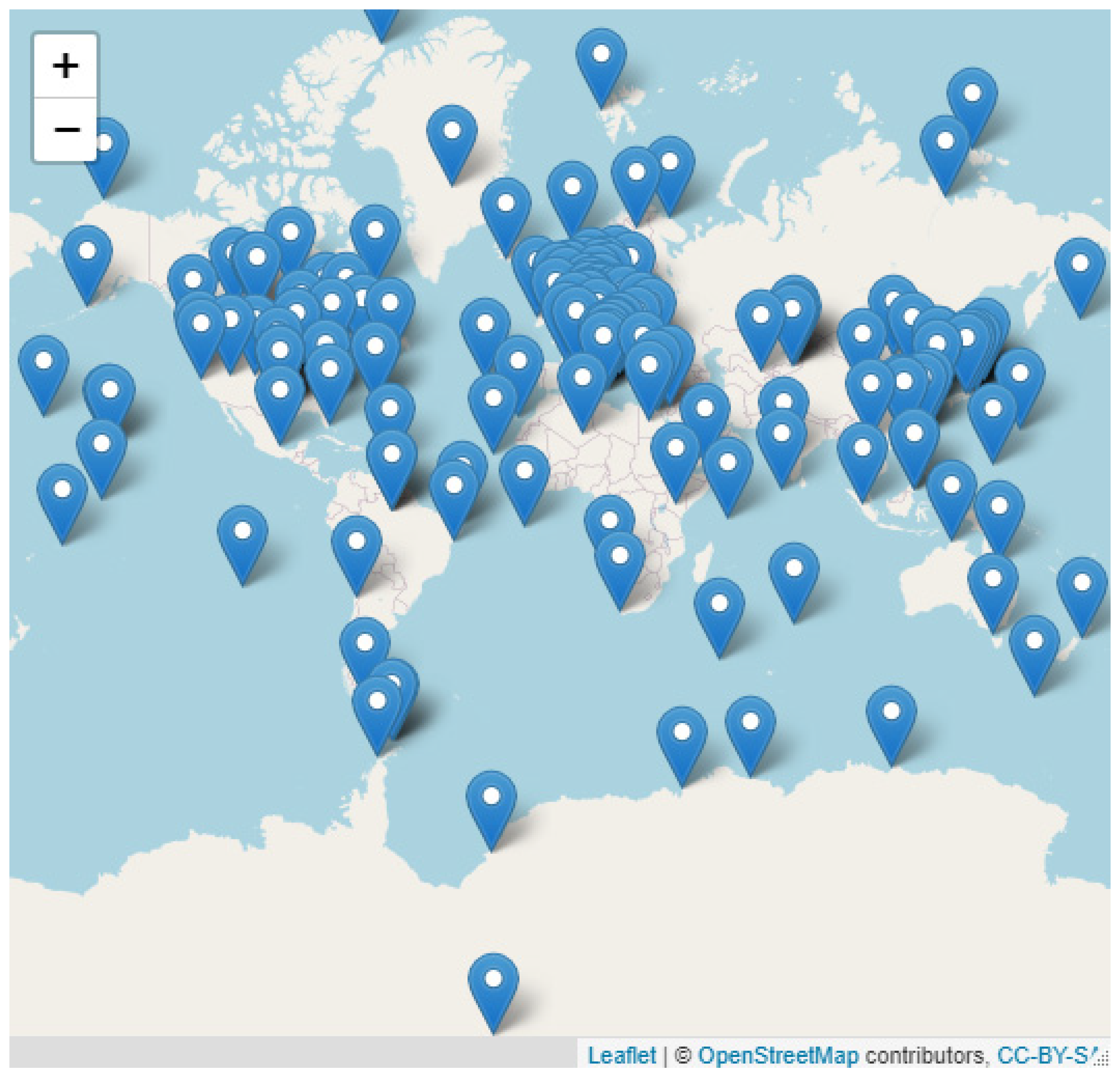
Figure 2.
Mean bias (MB) and RMSE (in ppmv) displayed by CO2 re-analysis product provided by CAMS-EAC4 in the comparison with worldwide in situ observation considered in this study. The compliance metric for each station can be accessed through the hypergraph available at (https://rpubs.com/danilocustodio/874273).

Figure 3.
The conditional quantile regression plot shows the comparison between CAMS reanalysis and observation. The observations are split up into bins according to the corresponding CAMS value. On the left, the conditional quantiles of CAMS are displayed again worldwide ground-based observations, which include the data from all stations considered in this study. On the right, the regression specimen for Barrow in Alaska (top right) and South Pole (bottom right) are shown. The median prediction line together with the 25/75th and 10/90th quantile values are plotted together with a line showing a “perfect model”. Also presented is a histogram of CAMS values (shaded grey) and a histogram of observed values (shown as a blue line).

Figure 4.
CO2 time series at Barrow (top) and South Pole (bottom) obtained from ground-based observa-tion and CAMS re-analysis. Both datasets are presented at a time resolution of 3 h.
Figure 4.
CO2 time series at Barrow (top) and South Pole (bottom) obtained from ground-based observa-tion and CAMS re-analysis. Both datasets are presented at a time resolution of 3 h.

Figure 5.
The annual CO2 cycle displayed by observation and CAMS includes all northern hemisphere sites considered at this study. The line represents the kernel average of the monthly concentration of CO2, and the shaded area represents its variance in a 95% significance interval.
Figure 5.
The annual CO2 cycle displayed by observation and CAMS includes all northern hemisphere sites considered at this study. The line represents the kernel average of the monthly concentration of CO2, and the shaded area represents its variance in a 95% significance interval.

Figure 6.
Diurnal cycle of CO2 (in ppmv) displayed by the observation (light blue) and CAMS (red). The blue panel shows the diurnal cycle at six stations with high CO2 mixing ratios variation; toward the left of the green panel, the diurnal variation at three remote stations with low CO2 fluxes is shown. The smooth line represents the kernel average of the diurnal concentration of CO2, and the shaded area represents its variance in a 95% significance interval.

Publisher’s Note: MDPI stays neutral with regard to jurisdictional claims in published maps and institutional affiliations. |
© 2022 by the authors. Licensee MDPI, Basel, Switzerland. This article is an open access article distributed under the terms and conditions of the Creative Commons Attribution (CC BY) license (https://creativecommons.org/licenses/by/4.0/).
Share and Cite
MDPI and ACS Style
Custódio, D.; Borrego, C.; Relvas, H. Worldwide Evaluation of CAMS-EGG4 CO2 Data Re-Analysis at the Surface Level. Toxics 2022, 10, 331. https://doi.org/10.3390/toxics10060331
AMA Style
Custódio D, Borrego C, Relvas H. Worldwide Evaluation of CAMS-EGG4 CO2 Data Re-Analysis at the Surface Level. Toxics. 2022; 10(6):331. https://doi.org/10.3390/toxics10060331
Chicago/Turabian StyleCustódio, Danilo, Carlos Borrego, and Hélder Relvas. 2022. "Worldwide Evaluation of CAMS-EGG4 CO2 Data Re-Analysis at the Surface Level" Toxics 10, no. 6: 331. https://doi.org/10.3390/toxics10060331
Note that from the first issue of 2016, this journal uses article numbers instead of page numbers. See further details here.