Combined Well Multi-Parameter Logs and Low-Flow Purging Data for Soil Permeability Assessment and Related Effects on Groundwater Sampling

Abstract

Cost-effective remediation is increasingly dependent on high-resolution site characterization (HRSC), which is supposed to be necessary prior to interventions. This paper aims to evaluate the use of low-flow purging and sampling water level data in estimating the horizontal hydraulic conductivity of soils. In a new quali-quantitative view, this procedure can provide much more information and knowledge about the site, reducing time and costs. In case of high heterogeneity along the well screen, the whole procedure, as well as the estimation method, could be less effective and rigorous, with related issues in the purging time. The result showed significant permeability weighted sampling, which could provide different results as the pump position changes along the well screen. The proposed study confirms this phenomenon with field data, demonstrating that the use of multiparameter well logs might be helpful in detecting the behaviour of low-permeability layers and their effects on purging and sampling. A lower correlation between low-flow permeability estimations and LeFranc test results was associated with high heterogeneity along the screen, with a longer purging time. In wells P43, MW08 and MW36, due to the presence of clay layers, results obtained differ for almost one order of magnitude and the purging time increases (by more than 16 min). However, with some precautions prior to the field work, the low-flow purging and sampling procedure could become more representative in a shorter time and provide important hydrogeological parameters such as hydraulic conductivity with many tests and high-resolution related results.

1. Introduction

In groundwater monitoring, site characterization is a complex process composed of many components and activities. It is carried on when a potential contamination threatens specific targets and should be necessary to provide background data on the site sensitivity to anthropogenic impact [1,2]. In situ monitoring plays a key role in groundwater protection and management, as it is the only way to find out reliable aquifer properties not only to assess the contamination but also to understand complex hydrogeological and hydro-chemical processes [3,4,5]. In particular, the assessment of porous aquifer vulnerability to contaminants and the eventual successful remediation measures are closely linked to the results of a well-performed groundwater monitoring, which in turn, depends on a highly structured well network, the field technicians’ skills and the financial resources of the involved stakeholders [6,7]. During these activities, well purging is usually a required and mandatory operation, carried out before groundwater sampling. Nowadays, low-flow purging and sampling is a well-known and consolidated methodology in environmental monitoring, consisting of pumping water at low flowrates (in fine-grained soils from 0.1 to 1 L/min) and minimizing the induced stabilized drawdown in the well (usually few tens of cm maximum) [8,9,10,11]. These limits are rather unstable for both practical and theoretical issues: stabilized low flowrates are not easy to set due to specific well conditions or pumps’ technical limits, and even with the lowest flow rate of the aforementioned range, particular hydrogeological settings with low-permeable soils does not allow in achieving acceptable low drawdowns. In addition, the defined ranges of “low-flow” conditions are strictly connected to the aquifer geometry and properties, which are sometimes unknown.

The misleading common belief is that the low-flow purging is only related to the pumped value, whereas one has to consider the induced groundwater flow to the well, which depends on the aquifer properties too [12,13,14]. In this sense, the only measured parameter that can give information about the right conditions is the drawdown ΔH, or even better the ratio ΔH/H (where H is the thickness of the aquifer), which allows to scale the drawdown taking into account the aquifer geometry also [15,16].

Regardless of the foregoing data that are strictly related to the hydraulics, the aim of this technique is mainly to correctly purge the well in order to obtain representative groundwater samples, with a reduced stress on the aquifer and less volumes of groundwater disposal at the same time. However, the word “representative” is still an object of discussion among scientists and practitioners, because representativeness often depends on the focus of the study, driven by specific compounds or related parameters [14,17,18].

The difficulty in collecting high-quality groundwater samples is related both to the specific sampling technique as well as the well construction and soil heterogeneity in terms of hydraulic conductivity. The presence of unknown low permeability layers or lenses in the aquifer may involve a contaminant back diffusion, modifying sample quality values over time [3,19,20,21,22]. Hence, collecting a formation water sample is always the main goal, but as the aquifer is heterogeneous and the screen length is sometimes not properly designed, the result of the operation will be always permeability-weighted sampling [23,24]. Consequently, the qualitative and quantitative aspects of low-flow purging and sampling cannot be separated and must be investigated more, in order to maximize the aquifer knowledge as well as the representativeness of the collected groundwater sample. The reduced time-steps of the site characterization process combined with the high resolution of the obtained results is crucial for stakeholders [25,26,27,28].

Recent studies demonstrated that this technique might be useful for estimating the horizontal hydraulic conductivity (K_H) of the aquifer and for strengthening the preliminary site assessment, without further and expensive investigations [15,29,30].

The variability of groundwater flow along the well screen and the presence of vertical flows may represent an issue [23,31,32]. This is mainly due to soil heterogeneities along the screen that affects both the evaluated K_H (a depth-weighted value) and the groundwater sample characteristics (permeability weighted). Recent studies show that vertical multiparameter well logs are a useful tool to assess soil heterogeneities and flow exchanges in the well water column [33,34]. For this reason, in this study, multi-parameter vertical logs combined with low-flow purging have been carried out in a landfill-monitoring network (17 monitoring wells), to achieve a more in-depth site characterization. The results obtained show that the use of a combined quali-quantitative approach could be helpful to understand the flow regime better along the screen well, identifying possible outliers of the low-flow proposed methodology for estimating aquifer K_H, due to low-permeability layers.

2. Study Area and Geological Framework

The study area is in Italy, in the landfill of Borgo Montello, few kilometres far from Latina, in the Latium Region (Figure 1). The location is in the southern portion of the Roman countryside and on the southern slopes of the volcanic region of the Alban Hills.

The related hydrographic basin is that of the Astura River, which overall extends for about 400 km². Its length, from the northern part, located in the highest area of the Alban Hills, is about 35 km. The Tyrrhenian Sea is about 10 km far from the study area, which is near the so called “Agro Pontino”, a swampy wetland area, currently reclaimed with an intense agricultural vocation and related high groundwater impacts [35].

The presence of these morphological features is interconnected with a complex regional geology, characterized by the pyroclastic soils and lavas of Alban Hills, whose boundaries are difficult to delimit because they have been covered by more recent alluvial soils towards the external part.

The “Agro Pontino” area represents a sector of the Plio-Pleistocene backdeep from the Volsci Range that characterizes the central part of the Tyrrhenian border of the Italian peninsula and for which important new studies have been performed at the regional tectonic level [36,37].

The intense subsidence allowed the sedimentation of marine deposits, mainly clayey formations, with a thickness of many hundreds of meters. Clayey formations, practically impermeable, can be considered the regional groundwater basement. Hence, pyroclastic rocks and tuffs, locally covered by sands, host the main aquifer of the area (Figure 2).

Their limited outcrop largely depends on the erosion process related to the overlying sands. The presence of silty clayey levels may constitute local aquitards, whereas the base aquiclude is related to the presence of the previously mentioned marine clay formations [38]. The landfill site is located few kilometres far from the small town of Borgo Montello. It is divided in two waste disposal basins, protected by underground hydraulic barriers (black contours in Figure 2) and surrounded by the monitoring well network, consisting of 17 points. The well depths are between 14.5 (minimum) and 41 m (maximum), whereas monitoring point elevations range from 11 to 29.19 m asl. (

Table 1. Coordinates (WGS84) and depth of the landfill monitoring wells.

ID	N-WGS84 (°)	E-WGS84 (°)	Depth (m)	Altitude (m asl)	Depth to Water (m)	Water Table (m asl)
MW1	41.4855	12.7661	34.0	28.11	13.7	14.41
MW2	41.4861	12.7635	20.0	22.76	8.8	13.96
MW8	41.4853	12.7678	40.0	28.58	15.8	12.78
MW15	41.4858	12.7711	41.0	28.77	15.6	13.17
MW31	41.4859	12.7641	30.0	23.19	10.4	12.79
MW17	41.4833	12.7695	37.0	22.22	9.3	12.92
MW19	41.4834	12.7627	36.0	29.19	17	12.19
MW20	41.4834	12.7639	25.0	24.86	14	10.86
MW21	41.4836	12.7587	20.0	11.04	1.3	9.74
MW22	41.4830	12.7583	14.5	11.23	1.2	10.03
MW33	41.4848	12.7597	30.0	32.6	21.8	10.8
MW35	41.4831	12.7610	30.0	25.17	14.4	10.77
MW36	41.4814	12.7681	33.0	26.88	14.7	12.18
MW37	41.4825	12.7697	37.0	28.99	16.2	12.74
MW38	41.4822	12.7658	40.0	28.41	16.8	11.56
MWE6	41.4805	12.7654	32.0	25.19	13.8	11.39
P43	41.4816	12.7615	33.5	26.70	15.87	10.83

). Based on the piezometric surveys previously carried out, groundwater flow is locally directed NE-SW (Figure 2).

3. Materials and Methods

Instrumentation and Measurements

Monitoring and field data collection have been carried out in March 2022, from the 28th to the end of the month. Both the low-flow purging technique and the multi-parametric log measurements involved all the 17 monitoring wells around the landfill perimeter. The depth to water was measured before purging started, and it was measured again, during the procedure, at increasing time steps (1, 2, 4, 8, and 16 min) using a water level meter instrument. A low-flow rate was achieved using a 12 v Proactive Hurricane submersible pump with booster, allowing to obtain a minimum flow of 0.1 L/min (Figure 3).

Flow-rates values have been manually measured, using a graduated vessel at known volume and measuring the time to fill it. The values generally were within the usual range of 0.1–1 L/min, even if in some cases, it has been possible to obtain stabilization of both chemical-physical parameters and water level at higher flow-rates, due to the high permeability of layers. Water temperature (T), electrical conductivity (EC), pH, dissolved oxygen (DO) and Redox potential (ORP) were the groundwater chemical-physical parameters measured, at the same time steps of the drawdowns. Their stabilization was determined in the field using a HANNA HI7609829 probe and a flow cell, keeping groundwater with no air contact during the reading (Figure 3).

The ranges defined for parameters’ stabilization between two successive readings follow the specific thresholds suggested previously [39]. This allowed for the end of purging activities and the beginning of water sampling for laboratory analyses. Regarding the multiparameter logs, they have been executed with a Seba Hydrometrie 5 W MPS D8 Multiparameter probe. The depth measurement frequency was every one meter, waiting at each step for parameter stabilization (Figure 3). The stabilized water level measured in each well during the low-flow purging was used as an input data, as well as the well radius and depth, for assessing aquifer horizontal hydraulic conductivity K_H [15].

This methodology is mainly based on the Dupuit/Thiem theory for unconfined/confined aquifers and its assumptions for steady-state groundwater flow to a fully penetrated well, which are supposed to be better respected in such flow conditions. Due to the unknown value of the radius of influence, an iterative procedure is proposed using the empirical Sichardt’s formula. The whole process of calculation is represented as a flow-chart in Figure 4.

Vertical flows may be considered mostly null compared to the horizontal ones, so, more realistically, water can be assumed to move horizontally through the well screen length. The hypothesis becomes less true in the case of non-homogeneous and/or anisotropic aquifers with a series of overlapping low and high permeability layers, compromising K_H estimation results as well as the water sample characteristics. The aim of this study is to verify and to quantify this deviation of results coming from the proposed method, with the help of multiparameter well log measurements.

In

Table 2. Static depth to water (DTW) measurements, screen position and length, and stratigraphic data referred to monitoring points.

Well ID	DTW	Well Screen			Unit	Top	Bottom	Thickness
-	(m)	ZTOP (m)	ZBOT (m)	L (m)	-	(m)	(m)	(m)
MW33	21.82	6	30	24	pyroclastic soil	3.7	13.4	9.7
					silty sand	13.4	20	6.6
					pyroclastic soil	20	28.8	8.8
					silty sand	28.8	30	1.2
MW37	16.18	6	36.5	30.5	pyroclastic soil	6.9	36.5	29.6
MW17	9.3	6	32	26	silty sand	9.2	12	2.8
					pyroclastic soil	12	31.1	19.1
					silty clay	31.1	32	0.9
MW15	15.5	20	39	19	silty clay	10.7	20	9.3
					pyroclastic soil	20	30	10
					silty sand	30	39	9
MW35	14.34	3	30	27	silty sand	4.6	15.4	10.8
					pyroclastic soil	15.4	25	9.6
					silty sand	25	28.3	3.3
MW20	13.92	3	25	22	silty sand	2.1	15	12.9
					pyroclastic soil	15	22	7
					silty sand	22	24.3	2.3
MW19	17.58	4	33.5	29.5	silty sand	9.2	17.3	8.1
					pyroclastic soil	17.3	30	12.7
					silty sand	30	33.5	3.5
MW31	10.56	2.8	22	19.2	pyroclastic soil	2.8	5	2.2
					silty sand	5	12.9	7.9
					pyroclastic soil	12.9	26.5	13.6
MW02	8.78	15	20	5	silty clay	11.5	13	1.5
					pyroclastic soil	13	15	2
					pyroclastic soil	15	20	5
MW01	13.6	20	24	4	silty clay	8	20	12
					pyroclastic soil	20	24	4
MW08	15.75	18	34.6	16.6	silty clay	11.2	19.5	8.3
					pyroclastic soil	19.5	32.2	12.7
					silty sand	32.2	34.6	2.4
MW21	1.38	5	16.3	11.3	silty clay	5.1	10.1	5
					silty sand	10.1	16.3	6.2
MW22	1.19	3	13.5	10.5	silty sand	4	7.8	3.8
					pyroclastic soil	7.8	11.5	3.7
					silty sand	11.5	13	1.5
MW36	14.52	10	33	19.5	silty sand	6	16.4	10.4
					pyroclastic soil	16.4	31.5	15.1
					silty sand	31.5	33	1.5
P43	15.87	12.7	33.5	20.8	silty sand	14.7	23	8.3
					pyroclastic soil	23	26.4	3.4
					silty sand	26.4	30	3.6
					silty clay	30	33.5	3.5
MWE6	13.61	12.5	32	19.5	silty sand	11.2	20.4	9.2
					pyroclastic soil	20.4	23.7	3.3
					silty sand	23.7	28.8	5.1
					silty clay	28.8	32	3.2
MW38	15.8	10	40	30	silty clay	16.1	20.1	4
					pyroclastic soil	20.1	32.7	12.6
					silty sand	32.7	40	7.3

, the main data referring to stratigraphy (top and bottom of the main geological layers), aquifer thickness and well construction information (well depth, screen length and position) are presented for each monitoring point of the well network. The main geological formations are pyroclastic soils, silty sands and silty clays, whose average K_H values are known from previous LeFranc tests carried on in the same site or from literature (pyroclastic soil: 2 × 10⁻⁵ m/s; silty sands: 1 × 10⁻⁶ m/s; and silty clays: 1 × 10⁻⁸ m/s).

Data presented in Table 2 show that, in the study area, the main aquifer is both in confined and unconfined conditions, requiring a double approach for the procedure of K_H estimation, as represented in Figure 4. The choice of the aquifer type is simply defined by comparing the depth to water (DTW) value and the well screen top (Z_TOP).

4. Results

The results obtained for saturated hydraulic conductivity coming from low-flow purging (K_LOW) are reported in

Table 3. Total K_H results obtained for low-flow purging (K_LOW) and LeFranc (K_LEF) for monitoring wells. The red values are for confined conditions while the black values are for unconfined conditions.

Well ID	KLEF (m/s)	KLOW (m/s)	Q (L/min)	Q (m3/s)	ΔH (m)	Q/ΔH (m2/s)	ΔH/H (−)
MW33	1.72 × 10−5	1.01 × 10−5	2	3.33 × 10−5	0.28	1.19 × 10−4	0.03
MW37	2.00 × 10−5	1.74 × 10−5	2	3.33 × 10−5	0.06	5.56 × 10−4	0.00
MW17	1.69 × 10−5	1.22 × 10−5	2	3.33 × 10−5	0.06	5.56 × 10−4	0.00
MW15	1.10 × 10−5	1.37 × 10−5	2	3.33 × 10−5	0.15	2.22 × 10−4	0.01
MW35	1.41 × 10−5	8.35 × 10−6	2	3.33 × 10−5	0.19	1.75 × 10−4	0.01
MW20	1.38 × 10−5	1.55 × 10−5	2	3.33 × 10−5	0.12	2.78 × 10−4	0.01
MW19	1.59 × 10−5	9.56 × 10−6	2	3.33 × 10−5	0.13	2.56 × 10−4	0.01
MW31	1.82 × 10−5	1.09 × 10−5	2	3.33 × 10−5	0.14	2.38 × 10−4	0.01
MW02	2.00 × 10−5	2.98 × 10−5	2	3.33 × 10−5	0.15	2.22 × 10−4	0.03
MW01	2.00 × 10−5	1.60 × 10−5	2	3.33 × 10−5	0.40	8.33 × 10−5	0.10
MW08	1.70 × 10−5	5.15 × 10−6	2	3.33 × 10−5	0.22	1.52 × 10−4	0.01
MW21	5.58 × 10−7	3.94 × 10−7	0.3	5.00 × 10−6	0.65	7.69 × 10−6	0.06
MW22	8.81 × 10−6	1.46 × 10−5	1	1.67 × 10−5	0.05	3.33 × 10−4	0.00
MW36	1.65 × 10−5	2.08 × 10−5	2	3.33 × 10−5	0.06	5.56 × 10−4	0.00
P43	4.47 × 10−6	1.51 × 10−5	2	3.33 × 10−5	0.07	4.76 × 10−4	0.00
MWE6	4.24 × 10−6	2.49 × 10−5	2	3.33 × 10−5	0.04	8.33 × 10−4	0.00
MW38	1.09 × 10−5	5.31 × 10−6	2	3.33 × 10−5	0.47	7.09 × 10−5	0.05

. They have been compared with values coming from Le Franc tests and averaged along the depth (K_LEF). Both values, in fact, are referred to average values weighted on different layer lengths along the well screen and below the water table, as the total horizontal hydraulic conductivity of the aquifer is expressed by using the following equation:

$${\mathrm{K}}_{\mathrm{H}}=\frac{{{\displaystyle \sum }}_{\mathrm{i}}{\mathrm{K}}_{\mathrm{i}}{\mathrm{h}}_{\mathrm{i}}}{{{\displaystyle \sum }}_{\mathrm{i}}{\mathrm{h}}_{\mathrm{i}}}$$

Four classes related to different correlation degrees have been defined, to quantify the number of wells in which K values, obtained with the proposed method, better match with the results of the LeFranc test, as follows:

• Low correlation for |K_LEF − K_LOW| > 1 order of magnitude (o.m.);
• Medium correlation for 0.5 < |K_LEF − K_LOW| < 1 o.m;
• High correlation for 0.25 < |K_LEF − K_LOW| < 0.5 o.m;
• Very high correlation for |K_LEF − K_LOW| < 0.25 o.m.

About 75% of the K values results showed a high correlation with the average LeFranc test results, whereas no results showed a low correlation, i.e., over 1 o.m. different (Figure 5a). In particular, poor results were obtained for MWE6, P43 and MW08 wells (medium class) and, to a lesser extent, for MW38 (high class) (Figure 5b).

Results from well multiparameter logs have been coupled with stratigraphy and low-flow purging data for each chemical-physical parameter measured. As expected, temperature (T) was not so useful to assess the heterogeneities, due to the slight changes of values along the screen as well as the almost immediate stabilization during the purging operation. Regarding dissolved oxygen (D.O.), the measured values were very different between the two different probes used for logs and purging, probably due to incorrect calibration; therefore, these values could not be compared.

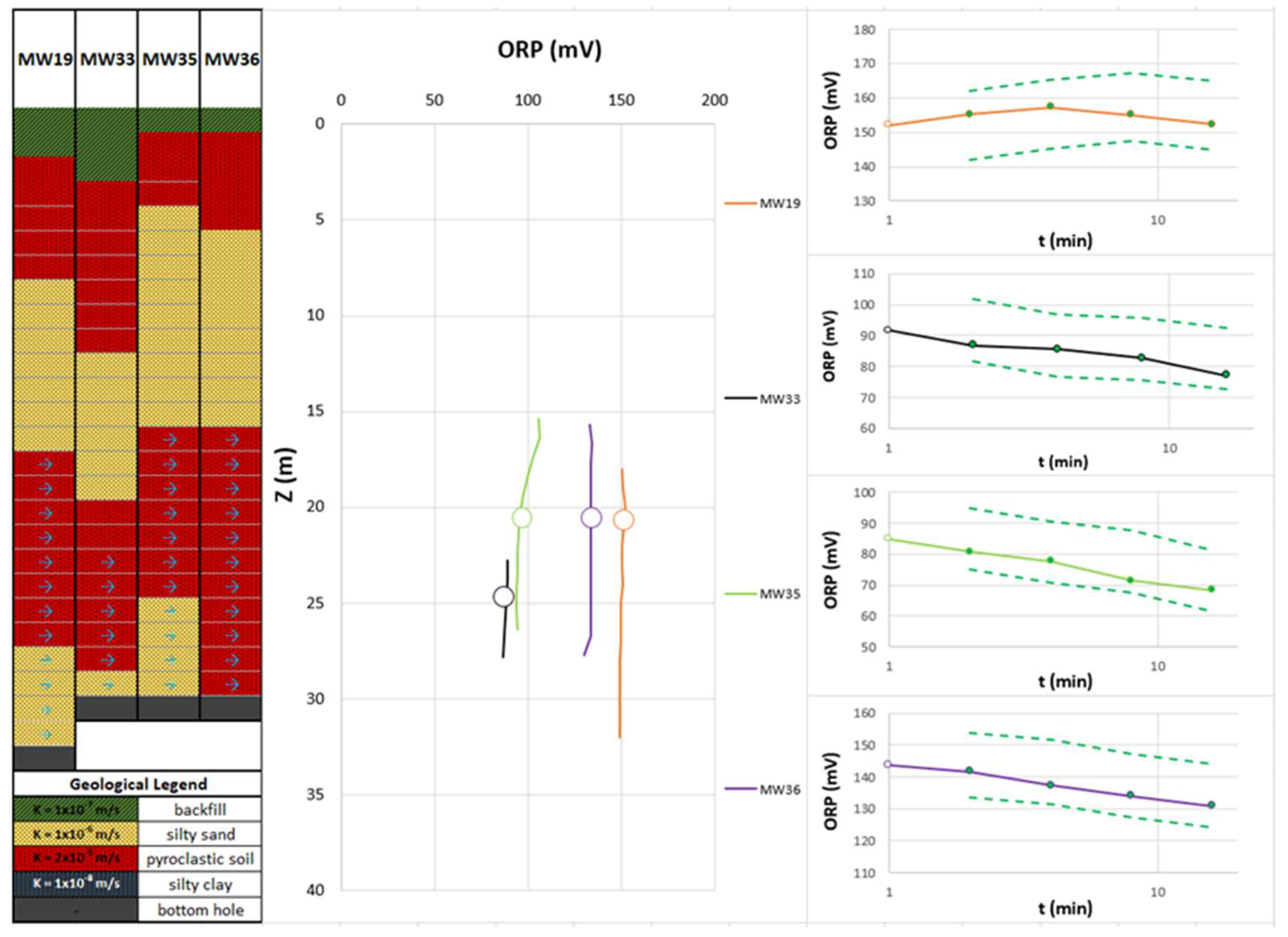
Hence, the base product of results obtained via this approach is presented in Figure 6, Figure 7 and Figure 8, where coupled logs and purging data are referred to EC, and pH and ORP parameters, respectively, for MWE6, P43, MW08 and MW38 wells. These wells present high soil heterogeneity along the screen. Figure 9, Figure 10 and Figure 11 present the results of wells with lower soil heterogeneity along the screen (MW19, MW33, MW35 and MW36).

In the left side of the layout, soil stratigraphy is represented for the different wells considered, as well as the screen length (grey horizontal lines) and the saturated zone (light blue arrows). Below this, a small geological legend contains soil types and permeability values of the geological formation (obtained using LeFranc tests). In the central chart, multiparameter log results are presented for wells taken into account.

The pump depth (coloured circle on the log trend) was about 20 m for each well (except for MW36) and can be considered as the “starting point” for the following step of measuring parameters during low-flow purging over time (right side of Figures). In the purging step, the stabilization of parameters was assumed to be obtained only when differences between two subsequent readings did not exceed the specific thresholds proposed previously [39].

To graphically show this aspect, two dashed green lines, representing the maximum and minimum values of stabilization criterion, outline the range of acceptance. The points falling outside this range are red coloured and indicate no stabilization of the specific parameter considered.

5. Discussion

The obtained results clearly show that low-flow purging piezometric data, collected during the groundwater monitoring activities, can be used for the assessment of horizontal hydraulic conductivity of the aquifer investigated. Almost 75% of the estimations highly match with the permeability values obtained from the LeFranc test results, calculated as a weighting average along the saturated zone of the well screen. Regarding the remaining 25% of values, even if the values showed lower correlations (high and medium), the deviations from the LeFranc test values were never greater than one order of magnitude (o.m.). Lower correlated results of the proposed methodology have been obtained in MWE6, P43, MW08 and MW31 wells, in which soil heterogeneity due to low-permeability layers along the well screen was much more marked. This fact is reflected by a sharp decrease or increase in some physical-chemical parameters at the interface between the low- and high-permeability layers, suggesting that both drawdown and parameter stabilization may become much more difficult in these conditions, especially depending on the pump position. This is confirmed by unstable parameter values measured during purging operations (Figure 6, Figure 7 and Figure 8), thereby highlighting that, even in high-permeability aquifers, as it is in this case study, the presence of thin low-permeability layers could affect the purging procedure in terms of time and costs. Instead, relatively homogeneous portions of the aquifer (maximum about 1 o.m. from layer to layer along the well screen) presented better results in terms of permeability (K_H) estimation and parameters’ stabilization (Figure 9, Figure 10 and Figure 11), showing almost vertical profiles of multi-parameter log results. Therefore, using these latter values, it is possible to correlate the geological heterogeneity with physical-chemical variation along the well screen, after which the pump position can be chosen to correctly intercept the main aquifer flow, sometimes not involving low-permeability layers and reducing the purging time a priori. In this study, pH was the most useful parameter for detecting layer K_H variations along the well screen, even if D.O. was not considered due to the issues related to instrumentation, as mentioned in Section 4.

Starting from the idea proposed by Harte et al. (2021) [40], who defined a heterogeneity factor (HF) for the use of his purging analyser tool (PAT), a new similar parameter has been defined in this study, considering not only the variability of permeability, but also the number of overlapping layers with different K_H and the saturated screen length. In this way, the heterogeneity is dependent on the monitoring well construction and the undisturbed groundwater level.

The heterogeneity factor along the well screen depends on the number of layers (i) and their permeability values (K), and it is defined as it follows:

$$F_H={\log }_{10}\left(\frac{\max K_i}{\min K_i}\right) ·\frac{i}{L_{SS}}$$

where L_SS is the saturated screen length, calculated as:

$$L_{SS}=\left\{\begin{array}{c}{L}_T \left(\mathrm{Confined}\right)\\ Z_{BOT}-DTW \left(\mathrm{Unconfined}\right)\end{array}\right.$$

Hence, the L_SS is the total screen length (L_T) in case of confined aquifer conditions, and equal to the difference between the bottom well depth (Z_BOT) and depth to water (DTW) in case of unconfined conditions.

The F_H calculated for monitoring wells and the correlation between the results coming from the LeFranc tests and the proposed method was good (Figure 12). Whether the stratigraphy is known, the use of this factor prior to the purging operations, even using approximate K_H values of geological layers, might help to individuate those monitoring wells where permeability estimation and physical-chemical parameter stabilization will be difficult to achieve.

6. Conclusions

Starting from previous research works that demonstrated the reliability of low-flow purging data for the estimation of soil horizontal hydraulic conductivity (K_H), this study aimed to focus on eventual weaknesses of the methodology proposed by De Filippi et al. (2020) [15] in the case of high geological heterogeneity along the well screen. Coupling drawdowns and depth multiparameter values obtained with well logs, the results showed that the precision of the proposed method is somehow related to both the geological heterogeneity and well screen design. In high-permeability aquifers, where also purging rates higher than 1 L/min can be used, the presence of low-permeability layers could affect both quantitative and qualitative results. Therefore, in the case of several overlapping layers with different K_H values, the position of the pump plays a key role in the precision of this parameter estimation, as well as in reducing/raising purging time, with a cascading effect on permeability-weighted samples collected. Multiparameter well logs, carried out before the procedure, could be very helpful to detect the interface between high- and low-permeability layers, usually suggested by a sharp decrease/increase in some specific parameters along the well screen. In this specific study, temperature (T) was not useful for the mentioned purposes, whereas pH was the best parameter for detecting the layers’ K_H variations along the well screen.

To support the procedure steps of low-flow purging and sampling, a heterogeneity factor, which takes into account both the soil and the screen characteristics as well as the geological features, has been defined. The use of this factor, prior to field work, can be helpful to know which monitoring wells require more attention, possibly with multiparameter log execution, or by being careful about the pumping depth that should be chosen based on well stratigraphy and screen knowledge.

Future studies will improve the knowledge of the K_H estimation technique using low-flow purging data as well as the parameters’ behaviour during the procedure in different hydrogeological contexts, continuing with a quali-quantitative approach. The position of the pump along the well screen and its effects should be furthermore studied and verified with measurements during the field work. The objective will be providing depth profiles of parameters changing over time during the low-flow purging and comparing them with the results of a dedicated FEM model.

References

- Preziosi, E.; Petrangeli, A.B.; Giuliano, G. Tailoring Groundwater Quality Monitoring to Vulnerability: A GIS Procedure for Network Design. Environ. Monit. Assess. 2013, 185, 3759–3781. [Google Scholar] [CrossRef] [PubMed]
- Chakraborty, A.; Prakash, O. Optimal Monitoring Locations for Identification of Ambivalent Characteristics of Groundwater Pollution Sources. Environ. Monit. Assess. 2022, 194, 664. [Google Scholar] [CrossRef]
- Ding, X.H.; Feng, S.J.; Zheng, Q.T. Forward and Back Diffusion of Reactive Contaminants through Multi-Layer Low Permeability Sediments. Water Res. 2022, 222, 118925. [Google Scholar] [CrossRef]
- Streeter, M.T.; Vogelgesang, J.; Schilling, K.E.; Burras, C.L. Use of High-Resolution Ground Conductivity Measurements for Denitrifying Conservation Practice Placement. Environ. Monit. Assess. 2022, 194, 784. [Google Scholar] [CrossRef] [PubMed]
- Oli, I.C.; Opara, A.I.; Okeke, O.C.; Akaolisa, C.Z.; Akakuru, O.C.; Osi-Okeke, I.; Udeh, H.M. Evaluation of Aquifer Hydraulic Conductivity and Transmissivity of Ezza/Ikwo Area, Southeastern Nigeria, Using Pumping Test and Surficial Resistivity Techniques. Environ. Monit. Assess. 2022, 194, 719. [Google Scholar] [CrossRef]
- Rivard, C.; Bordeleau, G.; Lavoie, D.; Lefebvre, R.; Malet, X. Can Groundwater Sampling Techniques Used in Monitoring Wells Influence Methane Concentrations and Isotopes? Environ. Monit. Assess. 2018, 190, 191. [Google Scholar] [CrossRef] [PubMed] [Green Version]
- Taheri, K.; Missimer, T.M.; Amini, V.; Bahrami, J.; Omidipour, R. A GIS-Expert-Based Approach for Groundwater Quality Monitoring Network Design in an Alluvial Aquifer: A Case Study and a Practical Guide. Environ. Monit. Assess. 2020, 192, 684. [Google Scholar] [CrossRef]
- Barcelona, M.J.; Varljen, M.D.; Puls, R.W.; Kaminski, D. Ground Water Purging and Sampling Methods: History vs. Hysteria. Gr. Water Monit. Remediat. 2005, 25, 52–62. [Google Scholar] [CrossRef]
- Kaminski, D. Low-Flow Groundwater Sampling: An Update on Proper Application and Use; Present Organised by EnviroEquip; QED Environmental Systems Inc.: Ann Arbor, MI, USA; Oakland, CA, USA, 2006. [Google Scholar]
- Robbins, G.; Higgins, M. Low Flow Sampling and Hydraulic Conductivity Analysis. Available online: https://www.epoc.org/resources/Documents/LowFlow6-5-18/Low%20Flow%20Lecture%20notes%206-5-18.pdf (accessed on 18 December 2022).
- Weaver, J.M.C.; Cavé, L.; Talma, A.S. Groundwater Sampling: A Comprehensive Guide for Sampling Methods; Water Research Commission: Gezina, South Africa, 2007; ISBN 9781770055452. [Google Scholar]
- Gomo, M.; Vermeulen, D.; Lourens, P. Groundwater Sampling: Flow-Through Bailer Passive Method Versus Conventional Purge Method. Nat. Resour. Res. 2018, 27, 51–65. [Google Scholar] [CrossRef]
- Qi, S.; Hou, D.; Luo, J. Optimization of Groundwater Sampling Approach under Various Hydrogeological Conditions Using a Numerical Simulation Model. J. Hydrol. 2017, 552, 505–515. [Google Scholar] [CrossRef]
- Wang, Y.; Hou, D.; Qi, S.; O’Connor, D.; Luo, J. High Stress Low-Flow (HSLF) Sampling: A Newly Proposed Groundwater Purge and Sampling Approach. Sci. Total Environ. 2019, 664, 127–132. [Google Scholar] [CrossRef] [PubMed]
- De Filippi, F.M.; Iacurto, S.; Ferranti, F.; Sappa, G. Hydraulic Conductivity Estimation Using Low-Flow Purging Data Elaboration in Contaminated Sites. Water 2020, 12, 898. [Google Scholar] [CrossRef] [Green Version]
- Sappa, G.; Filippi, F.M. De Quali-Quantitative Considerations on Low-Flow Well Purging and Sampling. Acque Sotter. Ital. J. Groundw. 2021, 10, 9–14. [Google Scholar] [CrossRef]
- Molofsky, L.J.; Richardson, S.D.; Gorody, A.W.; Baldassare, F.; Connor, J.A.; McHugh, T.E.; Smith, A.P.; Wylie, A.S.; Wagner, T. Purging and Other Sampling Variables Affecting Dissolved Methane Concentration in Water Supply Wells. Sci. Total Environ. 2018, 618, 998–1007. [Google Scholar] [CrossRef] [PubMed]
- Han, Y.L.; Tom Kuo, M.C.; Fan, K.C.; Lin, C.Y.; Chuang, W.J.; Yao, J.Y. Radon as a Complementary Well-Purging Indicator for Sampling Volatile Organic Compounds in a Petroleum-Contaminated Aquifer. Gr. Water Monit. Remediat. 2007, 27, 130–134. [Google Scholar] [CrossRef]
- You, X.; Liu, S.; Dai, C.; Guo, Y.; Zhong, G.; Duan, Y. Contaminant Occurrence and Migration between High- and Low-Permeability Zones in Groundwater Systems: A Review. Sci. Total Environ. 2020, 743, 140703. [Google Scholar] [CrossRef]
- Brooks, M.C.; Yarney, E.; Huang, J. Strategies for Managing Risk Due to Back Diffusion. Groundw. Monit. Remediat. 2021, 41, 76–98. [Google Scholar] [CrossRef]
- Borden, R.C.; Cha, K.Y. Evaluating the Impact of Back Diffusion on Groundwater Cleanup Time. J. Contam. Hydrol. 2021, 243, 103889. [Google Scholar] [CrossRef]
- Yang, M.; Annable, M.D.; Jawitz, J.W. Back Diffusion from Thin Low Permeability Zones. Environ. Sci. Technol. 2015, 49, 415–422. [Google Scholar] [CrossRef]
- McMillan, L.A.; Rivett, M.O.; Tellam, J.H.; Dumble, P.; Sharp, H. Influence of Vertical Flows in Wells on Groundwater Sampling. J. Contam. Hydrol. 2014, 169, 50–61. [Google Scholar] [CrossRef]
- Mcmillan, L.; Rivett, M.; Tellam, J.; Dumble, P.; Sharp, H. Water Quality Sample Origin in Wells under Ambient Vertical Flow Conditions. In Proceedings of the EGU General Assembly 2013, Vienna, Austria, 7–12 April 2013. [Google Scholar]
- Vienken, T.; Kreck, M.; Hausmann, J.; Werban, U.; Dietrich, P. Innovative Strategies for High Resolution Site Characterization: Application to a Flood Plain. Acque Sotter. Ital. J. Groundw. 2014, 3, 7–14. [Google Scholar] [CrossRef] [Green Version]
- Dijkshoorn, P.; Mori, P.; Zaffaroni, M.C. High Resolution Site Characterization as Key Element for Proper Design and Cost Estimation of Groundwater Remediation. Acque Sotter. Ital. J. Groundw. 2014, 3, 17–27. [Google Scholar] [CrossRef]
- Liu, G.; Butler, J.J.; Reboulet, E.; Knobbe, S. Bestimmung von Vertikalprofilen Der Hydraulischen Durchlässigkeit Mit Direct Push-Methoden. Grundwasser 2012, 17, 19–29. [Google Scholar] [CrossRef]
- Liu, G.; Butler, J.J.; Bohling, G.C.; Reboulet, E.; Knobbe, S.; Hyndman, D.W. A New Method for High-Resolution Characterization of Hydraulic Conductivity. Water Resour. Res. 2009, 45, 1–6. [Google Scholar] [CrossRef] [Green Version]
- Aragon-Jose, A.T.; Robbins, G.A. Low-Flow Hydraulic Conductivity Tests at Wells That Cross the Water Table. Ground Water 2011, 49, 426–431. [Google Scholar] [CrossRef]
- Robbins, G.A.; Aragon-Jose, A.T.; Romero, A. Determining Hydraulic Conductivity Using Pumping Data from Low-Flow Sampling. Ground Water 2009, 47, 271–286. [Google Scholar] [CrossRef]
- Harte, P.T. In-Well Time-of-Travel Approach to Evaluate Optimal Purge Duration during Low-Flow Sampling of Monitoring Wells. Environ. Earth Sci. 2017, 76, 251. [Google Scholar] [CrossRef]
- Mcmillan, L.A.; Michael, O.; Tellam, J.H.; Birmingham, B. Groundwater Quality Sampling at Contaminated Sites: The Long and the Short of It. Available online: https://www.envirotech-online.com/article/water-wastewater/9/in-situ-inc/groundwater-quality-sampling-at-contaminated-sites-the-long-and-the-short-of-it/1827 (accessed on 18 December 2022).
- Sappa, G.; Grelle, G.; Ferranti, F.; De Filippi, F.M. Temperature Logs to Evaluate Groundwater-Surface Water Interaction (Sabato River at Avellino, Campania). Rend. Online Soc. Geol. Ital. 2019, 47, 108–112. [Google Scholar] [CrossRef]
- Vitale, S.A.; Robbins, G.A. Characterizing Groundwater Flow in Monitoring Wells by Altering Dissolved Oxygen. Groundw. Monit. Remediat. 2016, 36, 59–67. [Google Scholar] [CrossRef]
- Sappa, G.; Rossi, M.; Coviello, M. Effetti Ambientali Del Sovrasfruttamento Degli Acquiferi Della Pianura Pontina (Lazio). In Proceedings of the Aquifer Vulnerability and Risk 2nd International Workshop, Parma, Italy, 14–16 September 2005; pp. 1–16. [Google Scholar]
- Cardello, G.L.; Vico, G.; Consorti, L.; Sabbatino, M.; Carminati, E.; Doglioni, C. Constraining the Passive to Active Margin Tectonics of the Internal Central Apennines: Insights from Biostratigraphy, Structural, and Seismic Analysis. Geosciences 2021, 11, 160. [Google Scholar] [CrossRef]
- Alessandri, L.; Cardello, G.L.; Attema, P.A.J.; Baiocchi, V.; De Angelis, F.; Del Pizzo, S.; Di Ciaccio, F.; Fiorillo, A.; Gatta, M.; Monti, F.; et al. Reconstructing the Late Pleistocene—Anthropocene Interaction between the Neotectonic and Archaeological Landscape Evolution in the Apennines (La Sassa Cave, Italy). Quat. Sci. Rev. 2021, 265, 107067. [Google Scholar] [CrossRef]
- Boni, C.; Bono, P.; Calderoni, G.; Lombardi, S.; Turi, B. Indagine idrogeologica e geochimica sui rapporti tra ciclo carsico e circuito idrotermale nella pianura pontina (Lazio meridionale). Geol. App. Idrog. 1980, 15, 203–247. [Google Scholar]
- US EPA. Environmental protection agency region i low stress (low flow ) purging and sampling procedure for the collection of from monitoring. Environ. Prot. 1996, 1, 1–13. [Google Scholar]
- Harte, P.T.; Perina, T.; Becher, K.; Levine, H.; Rojas-Mickelson, D.; Walther, L.; Brown, A. Evaluation and Application of the Purge Analyzer Tool (PAT) to Determine In-Well Flow and Purge Criteria for Sampling Monitoring Wells at the Stringfellow Superfund Site in Jurupa Valley, California, in 2017; U.S. Geological Survey: Reston, VA, USA, 2021. [Google Scholar] [CrossRef]
Figure 1.
Borgo Montello landfill study area.
Figure 2.
Geological map and cross section of the landfill well monitoring network area.
Figure 3.
Instrumentation used for well purging and groundwater sampling in low-flow conditions: (a) 12 v battery and booster for pumping flow regulation; (b) water level meter and HANNA HI7609829 multiparameter probe.
Figure 4.
Flow-chart of the proposed methodology for KH estimation with low-flow purging.
Figure 5.
Correlation results between permeability values estimated with the low-flow methodology (KLOW) and values obtained with the LeFranc tests (KLEF).
Figure 6.
Layout of coupled log-purging (z-t) EC results for high-heterogeneity well types (MWE6, P43, MW8 and MW38).
Figure 7.
Layout of coupled log-purging (z-t) pH results for high-heterogeneity well types (MWE6, P43, MW8 and MW38).
Figure 8.
Layout of coupled log-purging (z-t) ORP results for high-heterogeneity well types (MWE6, P43, MW8 and MW38).
Figure 9.
Layout of coupled log-purging (z-t) EC results for low-heterogeneity well types (MW19, MW33, MW35 and MW36).
Figure 10.
Layout of coupled log-purging (z-t) pH results for low-heterogeneity well types (MW19, MW33, MW35 and MW36).
Figure 11.
Layout of coupled log-purging (z-t) ORP results for low-heterogeneity well types (MW19, MW33, MW35 and MW36).
Figure 12.
Graphical comparison between horizontal hydraulic conductivity precision and the proposed heterogeneity factor FH for each monitoring well.