Proposing a Wetland-Based Economic Approach for Wastewater Treatment in Arid Regions as an Alternative Irrigation Water Source

Abstract

Point and nonpoint wastewater sources have a detrimental, negative effect on agriculture, soil, surface, and groundwater supplies. In this research, a wastewater treatment system made up of a sedimentation tank, a horizontal subsurface flow constructed wetland (HSSF-CW), a vertical subsurface flow constructed wetland (VF-CW), and a storage tank was proposed, designed, and cost estimated. Small populations in underdeveloped nations with dry and semi-arid climates can use the treatment system as an affordable construction, maintenance, and operational solution for wastewater treatment. The system will protect agricultural lands and groundwater from pollution. The system can service 6000 capita and has a wastewater discharge of 780 m³/d in the developing arid region in El-Moghra Oasis western desert of Egypt, where the 1.5 million acres used for the land reclamation project based on groundwater irrigation. The relaxed tanks in a series model based on the areal loading rates and background pollutants concentrations (P-K-C*) was utilized to size the HSSF and VF-CWs. The results indicated that the HSSF-CW design treatment surface area was 2375 m², and the hydraulic surface loading (q) and hydraulic retention time (RT) were 0.33 m/d and 0.55 d, respectively, and utilizing Phragmites australis and Papyrus for the biological treatment. The expected overall cumulative removal efficiencies were 96.7, 70, and 100% for the biological oxygen demand (BOD), total phosphors (TP), and fecal coliforms (FC), respectively. The VF-CW indicates that there was a 2193 m² design treatment surface area, q = 0.36 m/d, and RT of 0.63 d. The expected BOD, TP, and FC removal efficiencies were 75, 33.3, and 92.7%, respectively. In order to simplify the design stages and the cost estimation, design and investment cost curves were established for a population range from 500 to 9000. The total monthly water loss due to evapotranspiration for the HSSF and VF-CWs indicates a range from 3.7 to 8.5%, respectively. The total investment cost analysis for the proposed system corresponding to 780 m³/d wastewater discharge of indicates a total investment cost of EUR 146,804 and EUR 24.46/per-capita equivalent (P.E). This approach can be used by decision makers in the Mediterranean region and Middle Eastern countries to improve the water quality using social and economic criteria, leading to the effective implementation of ecological restoration projects as a low-cost treatment system and adding a nonconventional water source that can be used in irrigation.

1. Introduction

Egypt is suffering from a scarcity of water supplies and increased rates of reused wastewater because of rapid urbanization, population growth, and the depletion of freshwater resources. According to the Egyptian Holding Company for Water and Wastewater [1], there is a demand for 114 km³/year water in Egypt, while there is only 60 km³/year of accessible water, of which the Nile River provides more than 90% of the country’s needs. Around 76% of Egypt’s water goes to the agricultural sector, with only 13% of it going to homes and 7% of it going to industries [2]. In this context, wastewater reuse can be a useful approach that can assist in addressing some of the future water demands for agriculture and other water-related issues.

Now, Egypt has 409 wastewater treatment facilities that serve 59.7% of the population, covering 90% of the country’s urban areas and 12% of its rural parts [3]. The Nile Delta has 289 wastewater treatment plants, which in sum have a total treatment capacity of 0.0087 km³/d, which is an amount the government aims to increase to about 0.019 km³/d by 2037 [4]. In addition, Egypt adopted a robust plan to directly repurpose agricultural drainage water for crop production or to mix it with freshwater in order to satisfy the increased water demands in various sectors [5,6,7,8]. In the Nile Delta, about 11 km³ of agricultural drainage water is reused each year [9]. In addition, about 5.0 km³ of domestic wastewater is produced in Egypt each year, most of which is drained and treated, or partially treated into agricultural drains [10].

If this domestic wastewater is not properly treated, it will have several effects that put the ecological function in danger [11]. One example of ecological harm brought on by the wastewater’s nutrient concentration is eutrophication [12]. It can also boost the growth of aquatic plants and decrease the amount of light that reaches the water body. In order to determine the best course of action, issues such as the cost (building, operation, and upkeep) and aesthetics must be taken into consideration. Additionally, because of their high rates of energy and mechanization, certain developing nations may not be able to apply a particular system [13]. Cost effectiveness and aesthetics are apparently essential factors in developing a treatment that is appropriate for the community at all times and in all places. For those reasons, it is crucial to treat wastewater effectively and efficiently. Today, CWs are utilized to enhance the quality of nonpoint and point sources of water pollution, such as residential wastewater, coal mine drainage, stormwater runoff, and agricultural wastewater [14,15]. Additionally, pretreated industrial wastewater from pulp and textile mills, paper mills, and seafood processing mills are treated using constructed wetlands along with fishpond discharges, compost, and landfill leachates, and compost and landfill leachates [16,17]. Constructed wetlands are the only method of treatment for some wastewaters, but for others, they are just one step in a longer process. Utilizing constructed wetlands (CWs) is one of the methods used to discover alternative treatments. Wetland plants, soils, and related bacteria are only a few examples of natural processes that are used in CW systems to treat wastewater [18]. The CW is a low-cost, low-maintenance technique that may be used in a variety of wastewater types [19,20]. They fit into small towns as well as major municipal systems in the final step of the wastewater treatment [21]. In addition, it has significant potential for being used in developing nations [22,23].

Constructed wetlands (CWs) are made up of shallow lagoons or channels (depths of less than 1 m) that are planted with local species that are typical of humid areas, in which the decontamination processes take place through interactions between the water, solid substrates, microorganisms, vegetation, and even fauna [24]. Based on the water circulation characteristics, constructed wetlands can be classified into surface and subsurface flows [25]. In contrast to surface flow wetlands, their subsurface equivalents admit higher organic loads, reduce the risk of contact with the population, and prevent the appearance of insects [26]. In the subsurface flow’s wetlands, a gravel bed serves as the substrate for plant development in subsurface artificial wetlands, and depending on the layout used, the wastewater runs either vertically or horizontally across the bed, acting as a biofilter [27]. A sizable number of additional physical, chemical, and biological processes, such as sedimentation, filtration, precipitation, adsorption, plant absorption, and microbial degradation, also occur in the bed [28].

Additionally, subsurface vertical flow constructed wetlands improve the nitrification capacity compared to those with a horizontal structure by enhancing oxygen transfer from the air to the wastewater flow [29]. However, the granular media is not continuously inundated since the pulsed water circulation is discontinuous. Wastewater treatment in constructed wetlands is a multi-step process that involves sedimentation, sorption, filtration, microbial decomposition, and plant uptake [30], each of which affects the others.

In both tropical and arid countries, constructed wetlands (CWs) are one method that has demonstrated high removal rates of nutrients and organic [31,32,33]. Numerous HSSF-CWs proposed, according to the research that has been conducted across the globe, offer treatments which meet the regional water quality [34,35]. The pollutants in wastewater are viewed from an economic and environmental perspective as externalities that need to be handled in order to appropriately internalize all of the costs and benefits of the new wastewater treatment technologies that are recommended. There is a significant amount of existing research on wastewater treatment costs which focus on the cost functions for treating wastewater. Some studies consider quality factors (such as the contaminants eliminated or the quality of the influent and effluent), while others merely consider the amount of wastewater that has been treated. While some studies approach the operation and maintenance costs by solely predicting the energy expenses, the others estimate all of the cost factors.

Based on sample data from 22 Spanish WWTPs, Molinos-Senante et al. [36] presented information on the overall operating and maintenance expenses for each of the following five categories: energy, staff, reagents, waste management, and maintenance. The staff, accounting for one-third of the overall costs, was determined to be the most crucial component. The next two most significant expenses are maintenance and energy prices at 21% and 18%, respectively. The expenses for waste management and reagents have comparable percentage weights, making up 15% and 14% of the overall costs, respectively. According to their research, the average cost of plants with nutrient removal systems is EUR 0.21/m³, with this dropping to EUR 0.18/m³ if plants do not them. The parametric approach has been utilized in numerous different investigations to create cost functions for wastewater treatment. These are predicated on the development of a functional relationship between the cost drivers (explanatory variables) and the expenses of wastewater treatment (the dependent variable).

The objective of this study was to propose, design, and cost estimate a wastewater treatment system comprised of a primary sedimentation tank, an HSSF-CW followed by a VF-CW, and a ground storage tank. This system will serve small populations in developing areas in arid and semi-arid climates. Additionally, it will protect agricultural lands and groundwater from pollution, and the treated wastewater can be utilized in irrigation purposes. The system is located in El-Moghra Oasis in the western desert of Egypt in new land reclamation and cultivation project of 1.5 million acres, where the irrigation water is based on groundwater resources [37]. The system services 6000 inhabitants and has a wastewater discharge of 780 m³/d. To achieve the study objective, (i) we proposed a feasible design approach, and a cost estimation for a wastewater treatment system, (ii) we collected the data regarding the climate, wastewater discharge, and influent pollutants concentration in the study area, (iii) the P-k-C* relaxed tanks in series were utilized to design the proposed HSSF-CW and VF-CW to remove the BOD, TP, and FC pollutants in light of the treated wastewater regulations in Egypt, and (iv) a mathematical model to compute the HSSF and VF-CW areas and removal efficiency was constructed and solved using an Excel sheet based on the influent discharge (Q), the inlet pollutant concentration (Ci), the first-order areal rate coefficient ($Ka$), the background concentration (C*), the number of RTS (P), and C was the effluent target for the BOD, TP, and FC inlet concentration removal, and (v) a design and investment cost curve for a population range of between 500 and 9000 was created for the treatment system application in similar regions in order to shorten the design phases and cost estimation analysis.

2. Materials and Methods

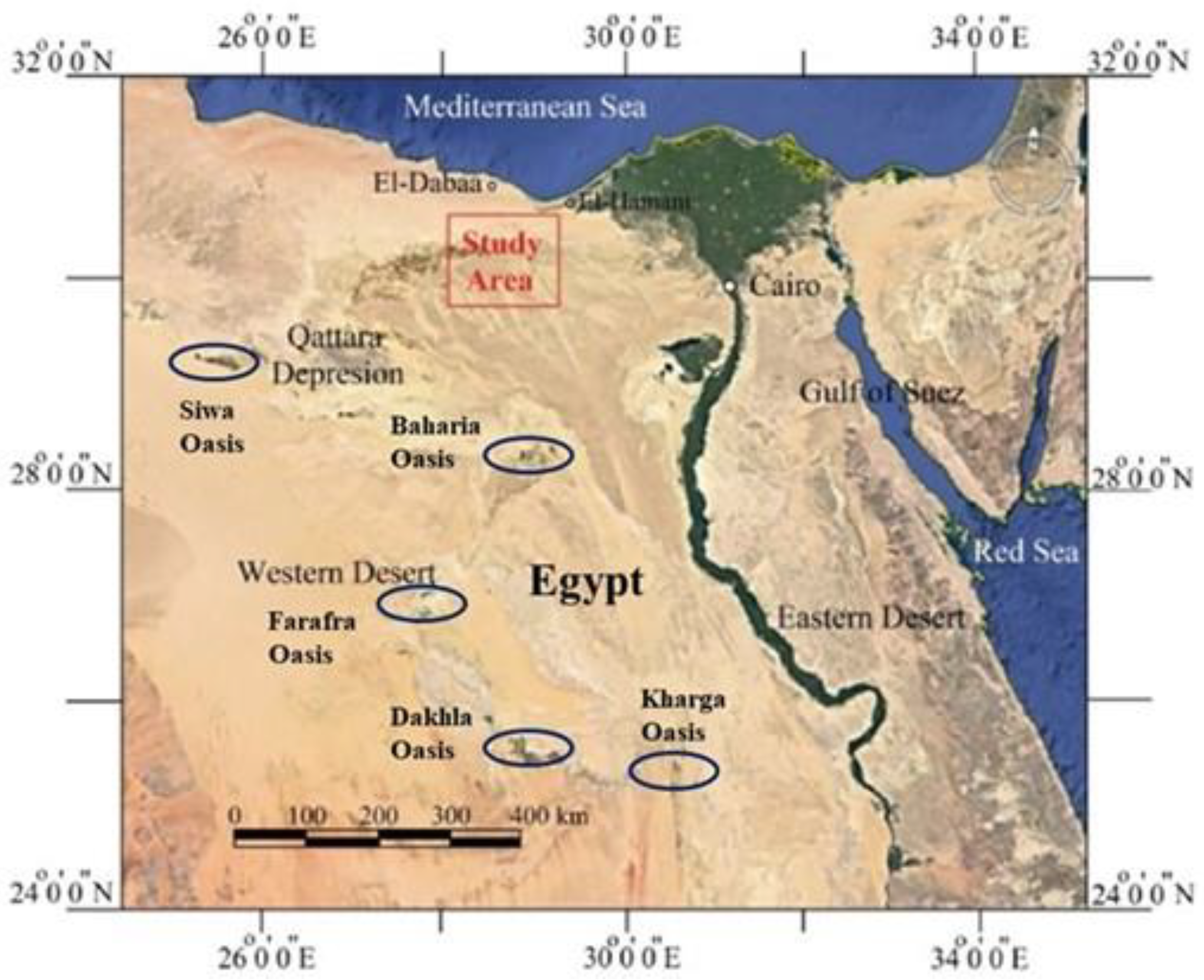
2.1. The Study Area

The study area is located in the El-Moghra Oasis western desert of Egypt. It is a part of the land reclamation project with the aim to reclaim 1.5 million acres, as shown in Figure 1. The projected cultivated area has 170 thousand acres. The winter crops are wheat, barley, and green beans, while the summer crops are sugar beet and maize. In addition, there are dates and olive trees. The project is based on groundwater wells [37]. The Ministry of Water Resources and Irrigation set sustainability guidelines for the well spacing, well depth, daily water withdrawal capacity from each well, submersible pump depth, and identifying the energy source used to power the well (solar energy). In addition, the agricultural and municipal runoff water should not be dumped outside of the project’s specified beneficiary areas, instead, it should be mixed with well water after the treatment processes. The climate data from the Dabaa station (western desert) between 1990 and 2020 were collected.

Therefore, the average minimum and maximum temperatures are 14.2 °C and 24.4 °C, respectively, and the average values of the wind speed, relative humidity, sunshine hours, solar radiation, reference evapotranspiration (ETo), and annual rainfall are 413 Km/d, 65%, 8.4 h, 18.9 MJ/m²/d, 4.61 mm, and 119 mm, respectively [38].

2.2. Water Quality Data

The proposed HSSF-CW is designed to service a population of 6000 people (farmers) in the village. A single well irrigated an area of around 230 acres, which is shared by ten farmers, each of whom lives in the village. There are often six family members living together in one home. The community has a population of roughly 6000 people, and its territory serves about 100 homes. The influent flow rate, 780 m³/d, is implied by the unit wastewater flow of 0.13 m³/capita/d. The BOD concentrations in the raw sewage water of 50 g/capita/d indicate a BOD concentration of 300 mg/L. In addition, the TN, TP, and FC influent concentrations are 35 mg/L, 10 mg/L, and 10⁷ Counts/100 mL, respectively. The effluent is made to comply with Egypt’s criteria [39] for wastewater reuse. The BOD and FC effluent concentrations are limited to 30 mg/L and 5000 Counts/100 mL, respectively. It is essential to perform the primary treatment prior to the HSSF-CW in order to reduce the amount of easily decomposable organic material that would otherwise accumulate in the wetland system’s entry zone, leading to blockages, odors, and adverse impacts on the entry zone’s plants. To accomplish this, similar technologies such as ponds, conventional primary treatment, Imhoff tanks, septic tanks, etc., can be used [11]. The main issue causing a mixed flow to occur in the HSSF-CW is media clogging [30].

Table 1. Influent and effluent pollutants concentrations during primary sedimentation stage.

Parameter	Unit	Influent Concentration Values	Effluent Concentration Values	Removal Efficiency (%)
COD	mg/L	600	420	30
BOD	mg/L	300	210	30
TP	mg/L	10	7	30
TN	mg/L	43	30	30.2
TSS	mg/L	1000	400	60
FC	Counts/100 mL	107	106	90

summarizes the influent and effluent pollutants concentrations during the primary sedimentation stage.

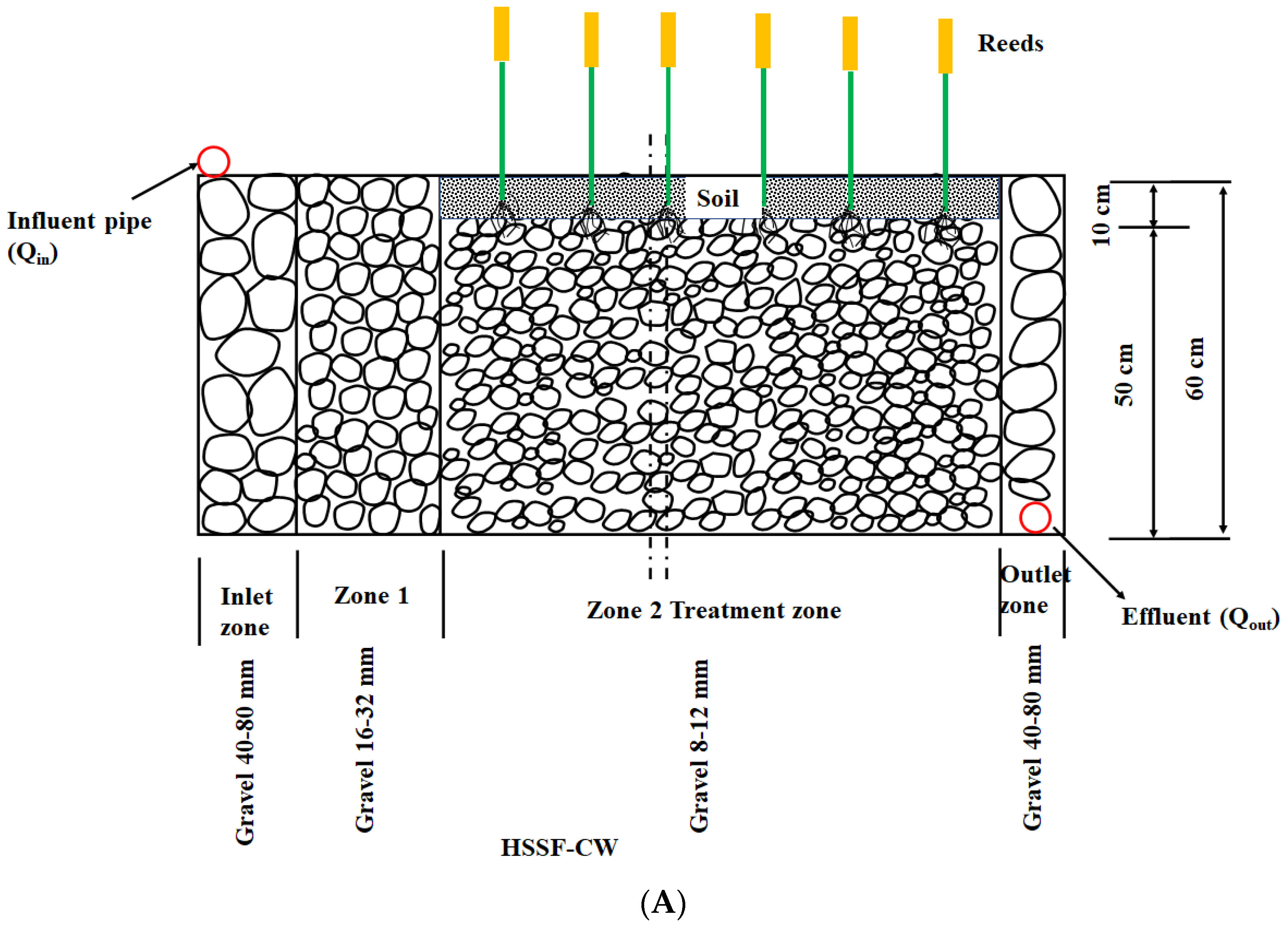
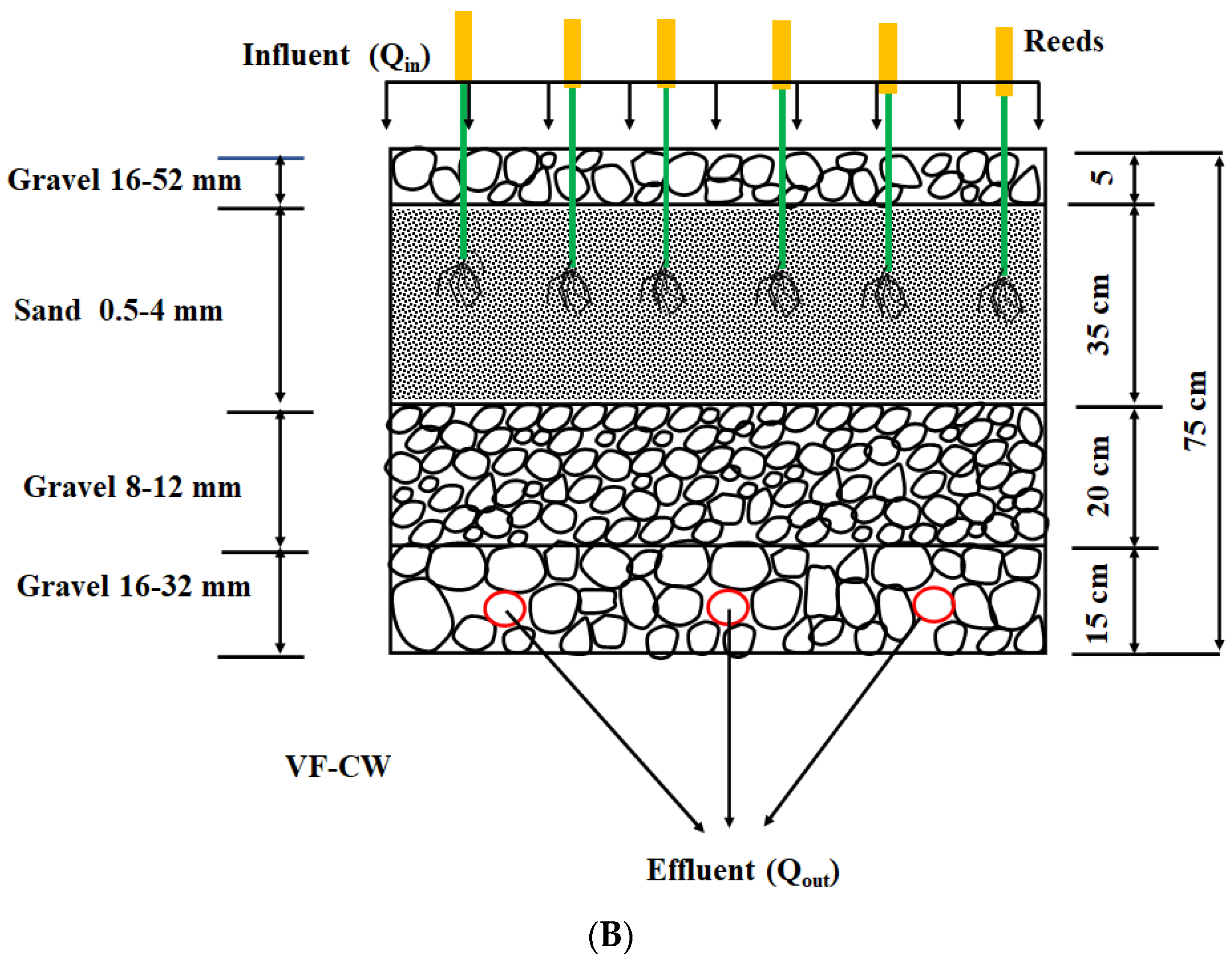
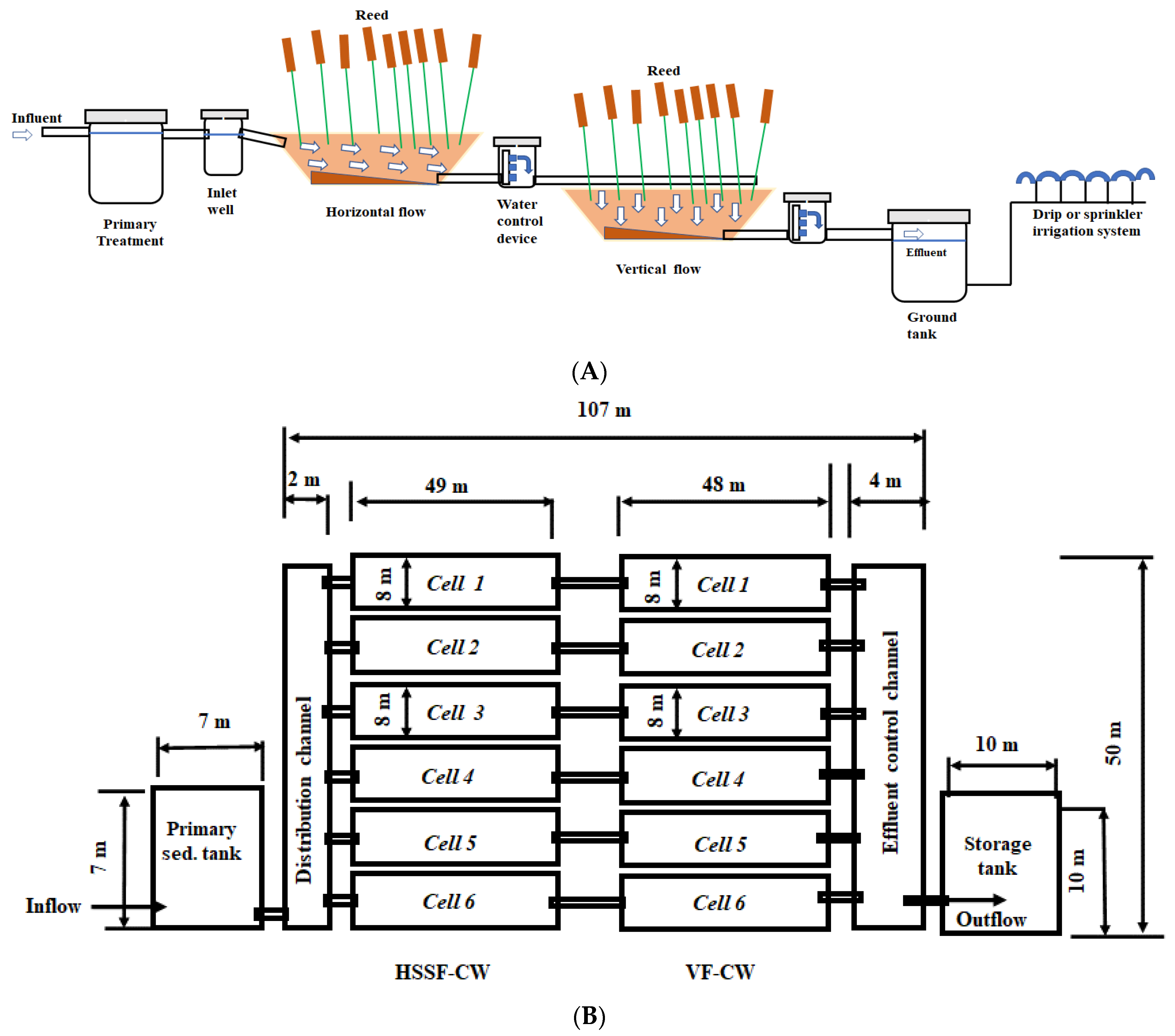
2.3. HSSF- and VF-CW’s Model Descrpition

In this study, the Continuous Stirred Tank Reactor (CSTR) model and the k-C* model are combined in the relaxed tanks in series (RTS) model (Equation (1)) to effectively explain both the pollutant depletion and the flow hydrodynamics [40,41,42]. This model takes into account steady state circumstances, which include no evapotranspiration, no infiltration, and a constant flow of the water in the wetland.

$$\left[\frac{C-C^{*}}{C_i-C^{*}}\right]=\frac{1}{{\left(1+\frac{Ka}{Pq}\right)}^P}$$

(1)

where C = effluent concentration, mg/L, $C^{*}$ = background concentration, mg/L, $C_i$ = influent concentration, mg/L, $P$ = apparent number of RTS, dimensionless, q = hydraulic loading rate, m/d, and $Ka$ = first-order areal rate coefficient, which is given by:

$$Ka=K_{20}{\theta }^{\left(T-20\right)}$$

(2)

$K_{20}$ is the removal rate constant at 20 °C (m/year), θ is the dimensionless temperature coefficient, and T is wastewater temperature in °C. In addition, the hydraulic residence time (RT) in days is given by:

$$RT=\frac{V}{Q}=\frac{Ay\phi }{Q}=\frac{y\phi }{q}$$

(3)

where $Q$ is the design discharge (m³/d); A is the surface area of the system (m²); V is the system volume (m³); y is the depth of flow (m); $\phi$ is the media porosity, which expresses the space available for the water to flow through the media, roots, and other solids in the HSSF-CW. In addition, the constructed wetland treatment efficiency (WE) is given as follows:

$$WE=\frac{C_i-C}{C_i}$$

(4A)

In the subsurface engineered wetland systems, Reed et al. [42] suggested that the organic loading should not go over a limit value of 10 g/m²/d. This relationship can be expressed as follows:

$$C_i Q/A\le 10$$

(4B)

2.4. Proposed HSSF and VF-CWs Construction Details

The HSSF-CW was selected as this kind of system does not have a clogging problem. The outlet flow comes from the primary sedimentation tank entering the HSSF-CW system (cell). The cell design comprises a rectangular bed that is surrounded by a 0.25 m masonry construction, the bed is lined by 10 cm of plain concrete or it is lined by geomembranes such as PVC sheets, which are durable, economical cost, and easily constructed, to prevent wastewater seepage. In this study, geomembrane lining was applied. Since the cell is 0.30 m above and 0.30 m below the earth, no groundwater from the natural ground surface can enter the cell. The cell in constructed wetland has a length-to-width ratio from 1:1 to 3:1. The wetland plants are Phragmites (Reeds) and Papyrus, the plant count is 9 per m². Figure 2A,B shows the details of the reed bed media to avoid blocking in the HSSF and VF-CWs, respectively [30]. The thickness of the bed media (gravel and sand) for the HSSF-CW is 60 cm, and it is 75 cm for the V-CW. Therefore, the HSSF-CW media bed consists of four zones: an inlet zone with a gravel size of 4–8 cm, zone 1 with a gravel size of 1.6–3.2 cm, zone 2 (treatment zone) with a gravel size of 0.8–0.12 cm, and finally, an outlet zone with a gravel size of 4–8 cm. On the other hand, the VF-CW media bed comprises of a top zone (inlet) with a gravel size of 1.6–5.2 cm, which is followed by the treatment layer with a sand size of 0.5–4 mm, and this sand is supported by a gravel layer which has a size of 0.8–1.2 cm, and finally, the bed layer has a gravel of size 1.6–3.2 mm. In addition, the bed slope for the HSSF and VF-CWs is adjusted by 1–2% so that wastewater would flow towards the effluent end. During the preparation stage, the water was added to the HSSF and VF-CWs to help the soil settle and encourage the growth of macrophytes.

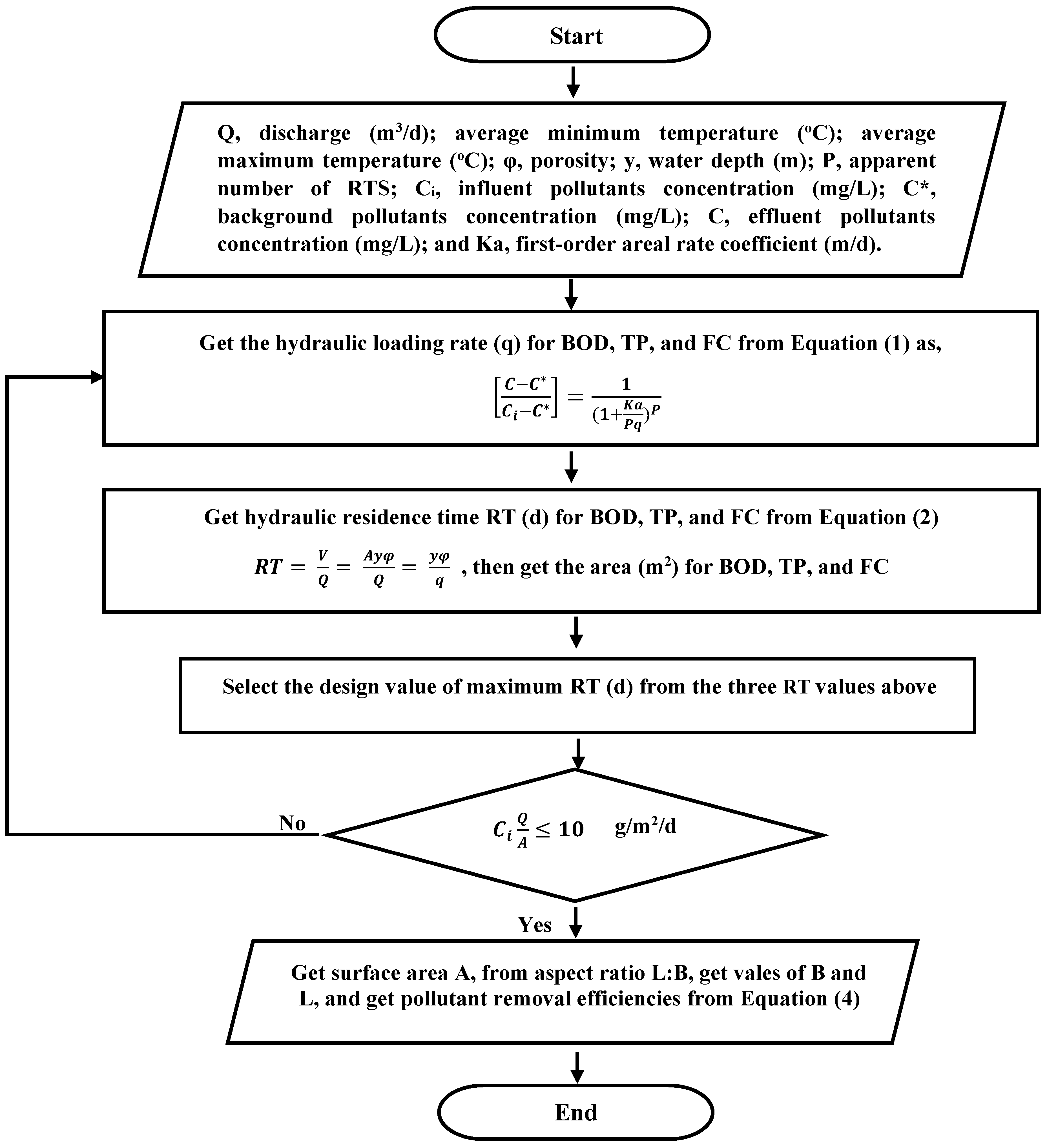
2.5. Modeling HSSF-CW and VF-CW Efficiencies Using the P-K-C*

The P-K-C* model, which is based on the relaxed tanks in series (RTS) flow model, is applied to design the HSSF-VF-CWs. Equation (1) is utilized to lower the inflow pollutants concentration to the desired level according to the wastewater treatment regulations in Egypt [39]. For the estimation of the area, the following variables are used: influent discharge (Q), the inlet concentration ($C_i$), the first-order areal rate coefficient ($Ka$), the background concentration (C*), and the number of RTS (P), and C is the effluent target for BOD, TP, and FC. The design discharge (Q) value is 780 m³/d, and the BOD, TP, and FC influent concentrations after primary sedimentation are 210 mg/L, 27 mg/L, and 10⁶ Counts/100 mL, respectively. In this study, the background pollutant concentrations and the removal rate constant at 20 °C were taken from similar HSSF-CWs which were developed by Rashed [43]. Therefore, for the BOD, TP, and FC, the background pollutant concentrations ($C^{*}$) are 1 mg/L, 0.119 mg/L, and 4 Counts/100 mL, respectively. Additionally, the $Ka$ values for BOD, TP, and FC are 0.662, 0.16, and 1.492 m/d, respectively. The water depth y = 0.6 m for the HSSF-CW and 0.75 m for the VF-CW, the media porosity φ = 0.3, the number of RTS, P = 3, and we apply Phragmites (Reeds) and Papyrus plants. A flow control device is used to divert the flow of the water. The CW sizing criteria are based on Egypt’s regulations guideline of no more than 60 mg/L BOD effluent [39].

Table 2. Model input data for the proposed wastewater treatment system as VF-CW after the HSSF-CW.

HSSF-CW
Q (m3/d)	Average Min. Temperature (°C)	Average Max. Temperature (°C)	$\mathit{\phi }$	Water Depth (m)	Apparent Number of RTS (P)	Influent Pollutants	${\mathit{C}}_{\mathit{i}}$	C*	C	$\mathit{K}\mathit{a}$ (m/d)	WE (%)
780	14.2	24.4	0.3	0.6	3	BOD (mg/L)	210	1	50	0.662	76.2
						TP (mg/L)	7	0.119	4.5	0.16	35.7
						FC (Counts/100 mL)	106	4	104	1.492	99
VF-CW
780	14.2	24.4		0.75	3	BOD (mg/L)	50	1	10	0.662	80
						TP (mg/L)	4.5	0.119	3.0	0.16	33.3
						FC (Counts/100 mL)	104	4	500	1.492	95

Q, discharge; $\phi$, media porosity; $C_i$, influent pollutant concentrations; C*, background pollutant concentrations; C, effluent concentrations; $Ka$, first-order areal rate coefficient; WE, removal efficiency.

summarizes the model input data for the proposed wastewater treatment system for the VF-CW and the HSSF-CW. In addition, the flow chart in Figure 3 shows the model steps to size the HSSF and VF-CWs and obtain the pollutants removal efficacies. The following steps are employed using an Excel spreadsheet:

• Use the input model data summarized in Table 2 and obtain the HSSF and VF-CWs areas for the BOD, TP, and FC by utilizing Equation (1).
• Obtain the hydraulic residence time (RT) from Equation (3).
• The design area is the area corresponding to the maximum RT in days.
• Determine the surface loading rate (q) from Equation (3).
• Obtain the length and width in (m) for the HSSF and VF-CWs based on an aspect length-to-width ratio of 1:1
• Divide the CW width into n cells based on a cell width of 8.0 m, and by doing so, the number of cells (n) = width/8.0.

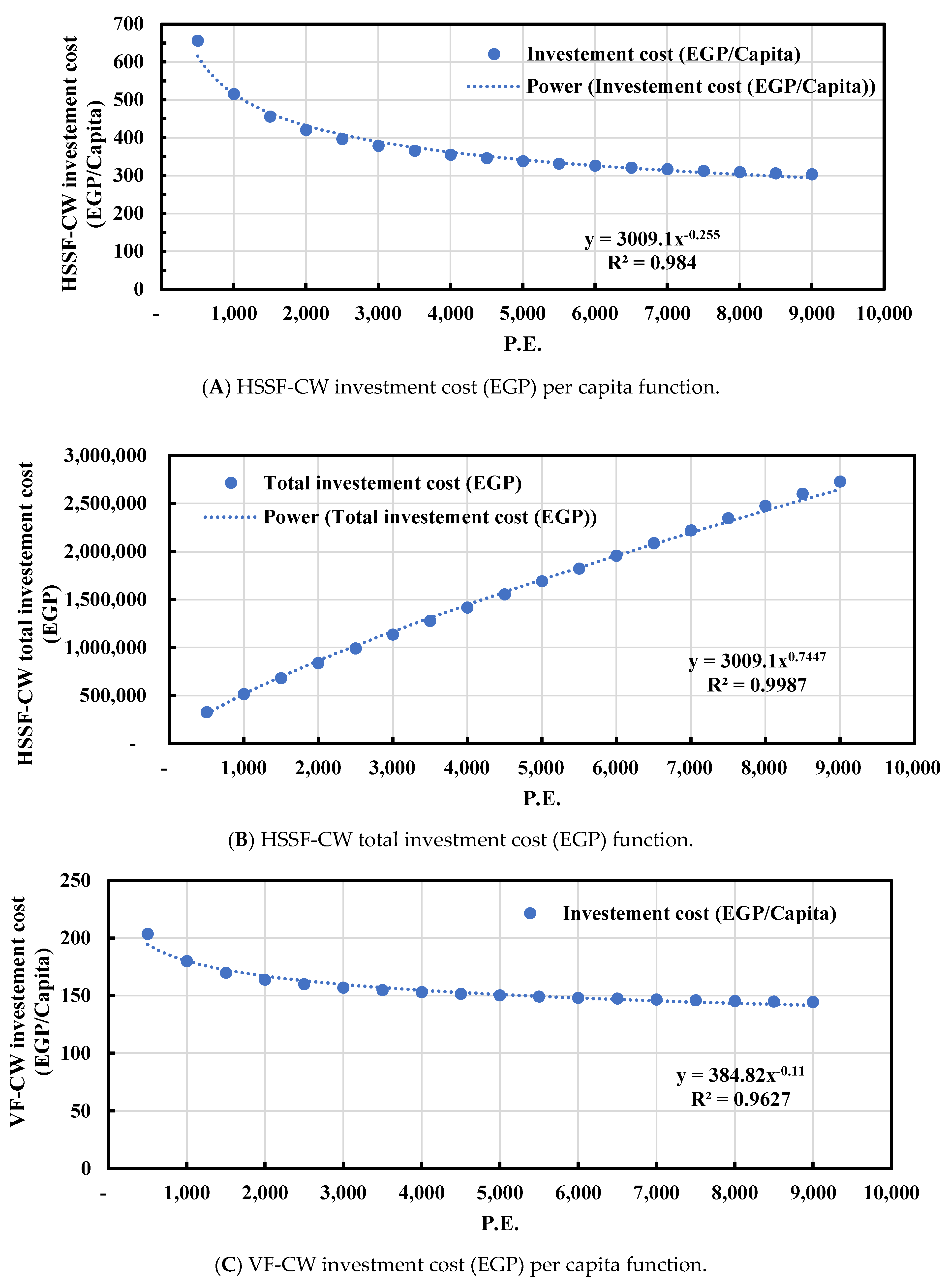
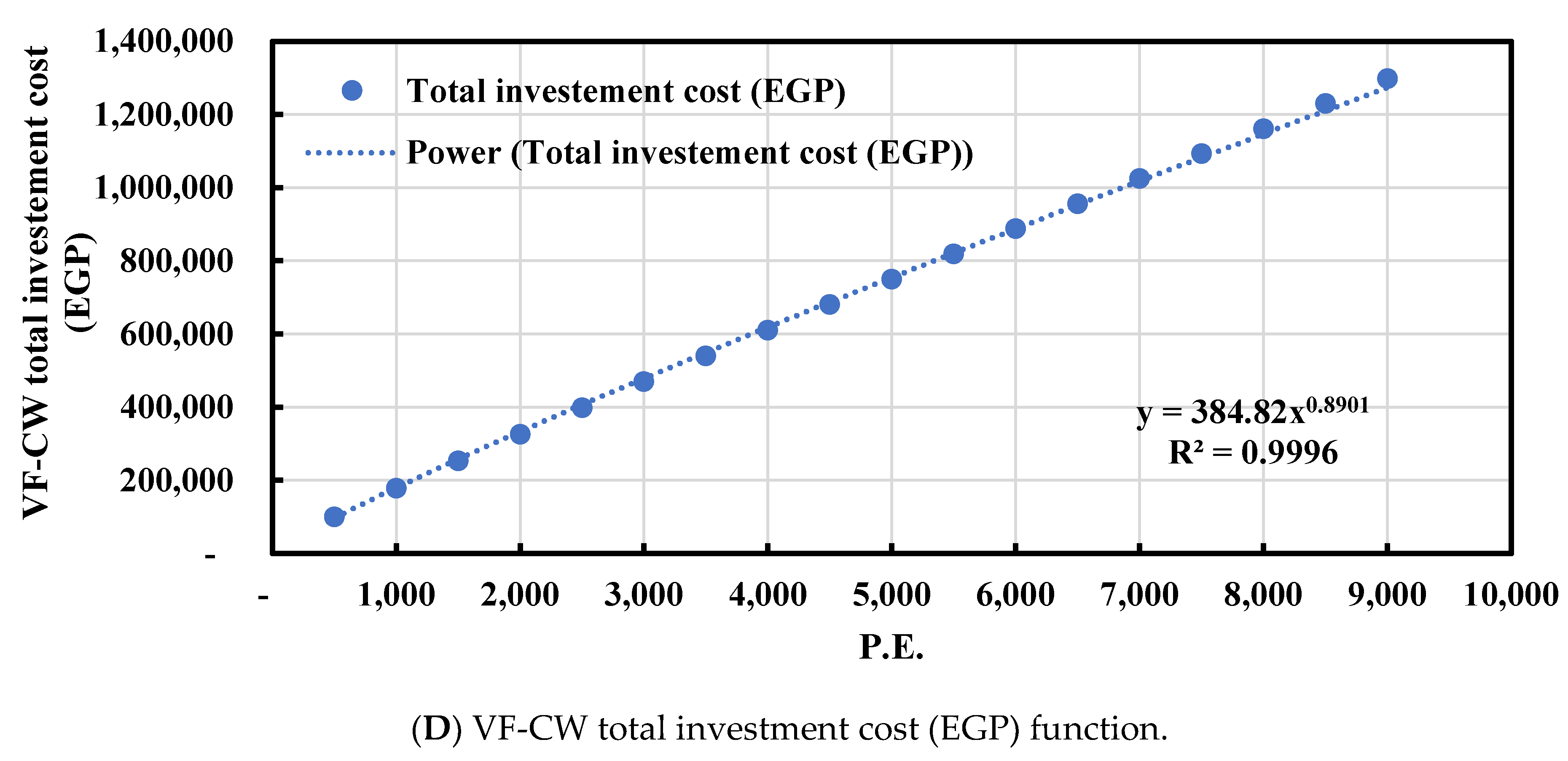
2.6. The Cost Function for Treating Wastewater

Numerous studies have examined the cost function of treating wastewater. Andreia et al. [44] and Molinos-Senante et al. [45] evaluated the costs of small, decentralized, energy-efficient wastewater treatment systems. They concentrated on secondary treatment procedures for small agglomerations (a population equivalent (P.E.) of 2000). The suggested cost function (in EUR per equivalent population) is for the investment and operating expenses of secondary wastewater treatment technology. Therefore, the cost for investment for constructed wetlands (Equation (5)) is:

$$\mathrm{Wetland} \mathrm{Investment} \mathrm{cost}, y=14.74x+3645.1$$

(5A)

$$\mathrm{Wetland} \mathrm{operation} \mathrm{and} \mathrm{maintenance} \mathrm{cost}, y=947.3x^{-0.188}$$

(5B)

where x is the P.E., and y is the total cost expressed as EUR/P.E. To ascertain the connection between the examined process’s inputs and outputs, the methodological foundation of the shadow prices is built on econometrics and optimization procedures [46]. Gkika et al. [47] conducted a design database of nine constructed wetlands (CW) facilities of various capacities (population equivalent (P.E.)), which was used to estimate the construction and operation costs, and then, to derive empirical equations relating to the required facility land area and the construction cost per the P.E. The total construction cost C (EUR 10³) is based on the contribution costs of the (i) inlet works, screening, (ii) Imhoff, settling, and sludge tank, (iii) first stage VF-CWs, (iv) second stage VF-CWs, (v) third stage HSSF or VF-CWs, (vi) sludge treatment bed, (vii) ancillary works (pipe network, siphon), (viii) disinfection (chlorination tank or maturation pond) (%), (ix) electrical, and (x) infrastructure and environmental restoration.

$$C=2827P{E}^{0.738}$$

(6A)

With a determination factor of R² = 0.97 and the total cost area ($A_t$) in ha:

$$A_t=4.9\times {10}^{-4} {\left(PE\right)}^{1.062}$$

(6B)

With a determination factor of R² = 0.97, the annual operating expense is EUR 17,853.74 or EUR 29.75 per P.E. or EUR 0.46 per m³. This operation cost consists of the following: salary for the facility operator (one person working part-time), electric energy costs for the pump operation for wastewater lifting and moving from one stage to another (e.g., all of the facilities), and the lighting for the facilities. For the computation, they used the values of EUR 127 for the electric energy per 1000 kWh and EUR 8 for operator hours.

3. Results

3.1. HSSF and VF-CWs Removal Efficiencies

Using an Excel spreadsheet to solve Equations (1)–(3) utilizing the input data summarized in Table 2, the results show that the proposed HSSF-CW design treatment surface areas for the BOD, TP, and FC are 2198, 2375, and 5712 m², respectively (

Table 3. Model output results for HSSF and VF-CWs.

HSSF-CW
	BOD	TP	FC
Area (m2)	2198	2375	5712
RT (d)	0.5	0.55	1.3
Surface load rate, q (m/d)	0.35	0.33	0.33
Efficiency (WE) (%)	76.2	35.7	99
Design values
Area (m2)	2375
RT (d)	0.55
Surface load rate, q (m/d)	0.33
Efficiency (WE) (%)	78.2	35.7	93.7
VF-CW
	BOD	TP	FC
Area (m2)	2648	2193	2700
RT (d)	0.77	0.63	0.78
Surface load rate, q (m/d)	0.29	0.36	0.36
Efficiency (WE) (%)	80	33.3	95
Design values
Area (m2)	2193
RT (d)	0.63
Surface load rate, q (m/d)	0.36
Efficiency (WE) (%)	75	35.7	92.7

BOD, biological oxygen demand; TP, total phosphors; FC, fecal coliforms; and RT, hydraulic retention time.

). The results show the area needed for the FC treatment is almost twice as large as the space needed for the TP therapy (2375 m²) (Table 3). Therefore, for economic purposes, we selected the design area of the HSSF-CW is 2375 m², with q = 0.33 m/d and the RT being 0.55 d. Consequently, the removal efficiencies in the HSSF-CW for the BOD, TP, and FC based on the design area (2375 m²) are 78.2, 35.7, and 93.7%, respectively, as shown in Table 3. This indicates an increase in the removal efficiency from 76.2 to 78.2%, on the other hand, FC efficiency decreased from 99% to 93.7%.

Therefore, in order to increase the FC removal efficiency, the outlet distribution channel is designed to be 4 m wide to utilize the solar hours in the disinfection of the FC [10,29,48]. Additionally, the proposed VF-CW design treatment surface area for the BOD, TP, and FC indicates areas of 2648, 2193, and 2700 m², respectively (Table 3), whereas the water hydraulic residence time (RT) is 0.77, 0.63, and 0.78 d for the removal efficiencies of 80, 33.3, and 95% for the BOD, TP, and FC, respectively. Therefore, for economic purposes, as previously in the HSSF-CW, the selected design area of the VF-CW is 2193 m², with q = 0.36 m/d and the RT being 0.63 d. The removal efficiencies in the VF-CW for the BOD, TP, and FC based on the design area (2193 m²) are 75, 35.7, and 92.7%, respectively. In addition,

Table 4. Effluent water quality of each treatment process.

Parameter	Unit	Influent Concentration Values	P.S Effluent	WE (%)	HSSF-CW Effluent	WE (%)	VF-CW Effluent	WE (%)	Overall Cumulative Efficiency WE (%)
BOD	mg/L	300	210	30	50	76.2	10	80.0	96.67
TP	mg/L	10	7	30	4.5	35.7	3	33.3	70.00
FC	Counts/100 mL	10,000,000	1,000,000	90	10,000	99.0	500	95.0	100.00

P.S, primary sedimentation; WE (%), removal efficiency; HSSF-CW, horizontal subsurface flow constructed wetland; VF-CW vertical subsurface flow constructed wetland.

shows the overall cumulative efficiencies of the treatment system, which are 96.7, 70, and 100% for the BOD, TP, and FC, respectively.

3.2. HSSF and VF-CWs Sizing Design Curves

To facilitate design steps for the HSSF and VF-CWs, design curves for a population range from 500 to 9000 (discharge range 65–1170 m³/d) have been established utilizing an Excel spreadsheet. The design curves comprise (i) the HSSF-CW and VF-CW discharge and area function; (ii) the discharge, number of cells, and length of cell functions; (iii) the investment cost (LE) per capita function; (iv) the total investment cost function. To obtain the wetland design area for the HSSF and VF-CWs over a discharge range from 65 to 1170 m³/d, the influent and effluent pollutants concentrations from Table 2 were substituted into Equations (1)–(3) using an Excel sheet.

The design curves in Figure 4 are based on the BOD, TP, and FC removal efficiencies of 78.2%, 35.7%, and 93.7%, respectively, for the HSSF-CW. Additionally, the VF-CW design curves are based on the removal efficiencies for the BOD, TP, and FC of 75, 33.3, and 92.7%, respectively. The results of HSSF-CW design dimensions are listed in

Table 5. HSSF-CW design dimensions for discharge range of 65–1170 m³/d.

P.E.	Wastewater Consumption (WC) (m3/C/d)	Discharge (Q) (m3/d)	HSSF-CW Area (m2)	Number of Cells (n)	Length of Cell (L) (m)	Width of Cell (B) (m)	Aspect Ratio for CW	Aspect Ratio for Cell
500	0.13	65	198	2	14.1	8	0.9	1.8
1000	0.13	130	396	2	19.9	8	1.2	2.5
1500	0.13	195	594	3	24.4	8	1.0	3.1
2000	0.13	260	792	3	28.1	8	1.2	3.5
2500	0.13	325	990	4	31.5	8	1.0	3.9
3000	0.13	390	1188	4	34.5	8	1.1	4.3
3500	0.13	455	1386	5	37.2	8	0.9	4.7
4000	0.13	520	1584	5	39.8	8	1.0	5.0
4500	0.13	585	1781	5	42.2	8	1.1	5.3
5000	0.13	650	1979	6	44.5	8	0.9	5.6
5500	0.13	715	2177	6	46.7	8	1.0	5.8
6000	0.13	780	2375	6	48.7	8	1.0	6.1
6500	0.13	845	2573	6	50.7	8	1.1	6.3
7000	0.13	910	2771	7	52.6	8	0.9	6.6
7500	0.13	975	2969	7	54.5	8	1.0	6.8
8000	0.13	1040	3167	7	56.3	8	1.0	7.0
8500	0.13	1105	3365	7	58	8	1.0	7.3
9000	0.13	1170	3563	7	59.7	8	1.1	7.5

, and they include a discharge range of 65–1170 m³/d. In addition, the VF-CW design dimensions are listed in

Table 6. VF-CW design dimensions for discharge range of 65-1170 m³/d.

P.E.	Wastewater Consumption (WC) (m3/C/d)	Discharge (Q) (m3/d)	HSSF-CW Area (m2)	Number of Cells (n)	Length of Cell (L) (m)	Width of Cell (B) (m)	Aspect Ratio for CW	Aspect Ratio for Cell
500	0.13	65	224	2	13.5	8	0.8	1.7
1000	0.13	130	366	2	19.1	8	1.2	2.4
1500	0.13	195	548	3	23.4	8	1.0	2.9
2000	0.13	260	731	3	27	8	1.1	3.4
2500	0.13	325	914	4	30.2	8	0.9	3.8
3000	0.13	390	1096	4	33.1	8	1.0	4.1
3500	0.13	455	1279	5	35.8	8	0.9	4.5
4000	0.13	520	1462	5	38.2	8	1.0	4.8
4500	0.13	585	1645	5	40.6	8	1.0	5.1
5000	0.13	650	1827	6	42.7	8	0.9	5.3
5500	0.13	715	2010	6	44.8	8	0.9	5.6
6000	0.13	780	2193	6	46.8	8	1.0	5.9
6500	0.13	845	2376	6	48.7	8	1.0	6.1
7000	0.13	910	2558	7	50.6	8	0.9	6.3
7500	0.13	975	2741	7	52.4	8	0.9	6.6
8000	0.13	1040	2924	7	54.1	8	1.0	6.8
8500	0.13	1105	3107	7	55.7	8	1.0	7.0
9000	0.13	1170	3289	7	57.4	8	1.0	7.2

, and they include a P.E. range from 500 to 9000 and a discharge range of 65–1170 m³/d.

Therefore, for a population equivalent of 6000 capita and a discharge value of 780 m³/d, the HSSF-CW design area is 2375 m² (Figure 4A); this area is divided into six cells (Figure 4B), and each cell is 8 m in width and 48.7 m in length, indicating a 1:1 rectangularity ratio. Consequently, the discharge (m³/d) and the HSSF-CW design area relationship function (linear equation) (Figure 4A) based on Table 4 are obtained by using Equation (7).

y = 3.0449 x + 0.2288

(7)

where y is the design area (m²), and x is the discharge (m³/d), with a determination coefficient of R² = 0.99. In addition, a relationship between the discharge and the number of cells based on a HSSF-CW aspect ratio of 1:1 is obtained by using Equation (8).

$$y=0.2024 x^{0.5095}$$

(8)

where y is the number of cells in (m), and x is the discharge (m³/d), with a determination coefficient of R² = 0.99. Additionally, a relationship between the discharge in m³/d and the cell length based on a rectangularity of 1:1 is obtained by using a power function in Equation (9):

$$y=1.7514 x^{0.4994}$$

(9)

where y is the HSSF-WC length of the cell, and x is the discharge (m³/d), with a determination coefficient of R² = 0.99. The results show that a design curve for the VF-CW for the discharge (m³/d) and the design area relationship function (linear equation) (Figure 4C) indicates:

y = 2.8002 x + 9.2157

(10)

where y is the VF-WC design area (m²), and x is the discharge (m³/d), with a determination coefficient of R² = 0.99. In addition, a relationship between the discharge (m³/d) and the number of cells based on a rectangularity ratio of 1:1 is obtained by using a power function (Figure 4D) that is as the same that in Equation (9).

Additionally, a relationship between the discharge and the cell length based on a rectangularity ratio of 1:1 is obtained by using a power function (Figure 4D) such as:

$$y=1.6706 x^{0.5005}$$

(11)

where y is the length of cell, and x is the discharge (m³/d), with a determination coefficient of R² = 0.99. Figure 4 shows the design curves for HSSF-CW and VF-CW treatment systems, (A) HSSF-CW population equivalent area function, (B) HSSF-CW population equivalent, number of cells, and length of cell functions, (C) VF-CW population equivalent area, and (D) VF-CW population equivalent, number of cells (n), and length of cell functions. In addition, Figure 5 shows a detailed drawings of HSSF-CW and VF-CW, (A) cross-section elevation and (B) plan. Therefore, the system is intended for a 780 m³/d flow rate, the constructed wetland has a length-to-width ratio of 1:1, and it is designed to be a plug flow reactor. The HSSF-CW indicates a rectangular bed of area 2375 m², which is divided into six cells, each cell is 48.7 m long and 8 m in width, and they house the common wetland plants Phragmites (Reeds) and Papyrus, which are the design element of this HSSF-CW.

In addition, the VF-CW has a rectangular bed of area 2193 m², which is divided into six cells, and each cell 46.8 m long and 8 m in width, and they house the common wetland plants Phragmites (Reeds) and Papyrus.

3.3. HSSF and VF-CWs Water Balance

Table 7. Monthly HSSF-CW water balance.

Month	Inflow (m3/d)	Rainfall (mm/d)	Rainfall (m3/d)	ETo (mm/d)	ETo (m3/d)	Outflow (m3/d)	Water Losses (%)
January	780	1.0	2.4	2.9	17.2	765.2	1.9
February	780	0.6	1.4	3.47	20.6	761.9	2.3
March	780	0.3	0.6	3.99	23.7	758.8	2.7
April	780	0.1	0.2	4.96	29.5	753.1	3.5
May	780	0.1	0.2	5.5	32.7	749.8	3.9
June	780	0.0	0.1	5.99	35.6	746.9	4.2
July	780	0.0	0.0	6.02	35.7	746.8	4.3
August	780	0.0	0.0	6.03	35.8	746.7	4.3
September	780	0.0	0.1	5.43	32.2	750.3	3.8
October	780	0.4	0.9	4.45	26.4	756.1	3.1
November	780	0.5	1.2	3.6	21.4	761.1	2.4
December	780	0.9	2.1	3.04	18.1	764.5	2.0

Total constructed wetland area is 2375 m².

and

Table 8. Monthly VF-CW water balance.

Month	Inflow (m3/d)	Rainfall (mm/d)	Rainfall (m3/d)	ETo (mm/d)	ETo (m3/d)	Outflow (m3/d)	Water Losses (%)
January	780	1.0	2.9	2.9	15.9	766.3	1.8
February	780	0.6	3.47	3.47	19.0	762.3	2.3
March	780	0.3	3.99	3.99	21.9	758.7	2.7
April	780	0.1	4.96	4.96	27.2	753.0	3.5
May	780	0.1	5.5	5.5	30.2	750.0	3.8
June	780	0.0	5.99	5.99	32.8	747.2	4.2
July	780	0.0	6.02	6.02	33.0	747.0	4.2
August	780	0.0	6.03	6.03	33.1	746.9	4.2
September	780	0.0	5.43	5.43	29.8	750.3	3.8
October	780	0.4	4.45	4.45	24.4	756.5	3.0
November	780	0.5	3.6	3.6	19.7	761.3	2.4
December	780	0.9	3.04	3.04	16.7	765.3	1.9

Total constructed wetland area is 2193 m².

summarize the water balance for the HSSF and VF-CWs, respectively. The monthly ETo and rainfall values were computed by the FAO-CROPWAT 8 model and its attached CLIMWAT 2 model to obtain the daily average climatic parameters at the Dabaa station (western desert), Egypt, from 1991 to 2020.

The soil in the study region is sandy, and the reed beds have a PVC membrane covering them (zero infiltration). In terms of the water balance (Equation (7)) yields for the HSSF-CW, the inflow discharge is 780 m³/d, whereas the outflow discharge ranges from 746.7 to 765.2 m³/d, and there is a monthly water loss of 1.9 to 4.3%. In addition, in terms of the water balance yields for the VF-CW, the inflow discharge is 780 m³/d, whereas the outflow discharge ranges from 746.9 to 766.3 m³/d, and the monthly water loss ranges from 1.8 to 4.2%. Therefore, the total monthly water loss for the HF and VF-CWs indicates a range from 3.7 to 8.5%.

4. Discussion

4.1. HSSF and VF-CWs Efficiencies

By comparing the results for the BOD, TP, and FC removal efficiencies in the HSSF-CW (78.2, 35.7, and 93.7%, respectively), the hydraulic residence time is 0.55 d, and the surface loading rate is 0.33 m/d according to previous work by the authors of [30,43,49,50], indicating that these are a good wetland operation condition.

Table 9. Comparison of the proposed HSSF-CW predicted removal efficiencies with monitored case studies.

Type of Wetland	Temp. (°C)	Plants	Discharge (m3/d)	Pollutants Concentrations		Removal Efficiency (%)	Surface Area (A) (ha)
				Inlet Flow (Ci) (mg/L)	Outlet Flow (C) (mg/L)
Proposed HSSF-CW	14.2–24.4	Phragmites australis and Papyrus	780	BOD = 210 TP = 7 FC = 106 (Counts/100 mL)	BOD = 46 TP = 4.5 FC = 6.3 $\times$ 106 (Counts/100 mL)	BOD = 78.2 TP = 35.7 FC = 93.7	0.2735
Proposed VF-CW	14.2–24.4	Phragmites australis and Papyrus	780	BOD = 46 TP = 4.5 FC = 104 (Counts/100 mL)	BOD = 11.5 TP = 2.9 FC = 4599 (Counts/100 mL)	BOD = 75 TP = 33.7 FC = 92.7	0.2193
HSSF-CW -Pilot scale in Karachi, NED University of Engineering and Technology [49]	20-36	Phragmites australis	1	BOD = 68.6 ± 23.6 TP = 7.6 ± 1.9 FC = 1.1 × 106 (Counts/100 mL)	BOD = 34.15 ± 15.5 TP = 3.7 ± 2.3 FC = 2.2 $\times$ 104 (Counts/100 mL)	BOD = 50 TP = 52 FC = 98	-
Lake Manzala reciprocating wetland system, Egypt [43]	14.1–27.8	Unplanted	250	BOD = 25 FC = 3342 (Counts/100 mL)	BOD = 4 FC = 153 (Counts/100 mL)	BOD = 84 FC = 95.4	0.0324
Agaa wastewater treatment, Delta of Egypt [30,50].	18	Phragmites australis and Papyrus	1500	BOD = 250	BOD = 60	BOD = 76	0.184

summarizes this comparison for the proposed HSSF and VF-CWs and their predicted removal efficiency with the monitored case studies. Therefore, for the Agaa HSSF wastewater treatment in the delta of Egypt, the BOD removal efficiency is 76%, which is very close to those of the proposed HSSF-CW (76%). By comparing the removal efficiency results for the HSSF-CW with those of Diana et al. [51], they studied the efficiency of subsurface constructed wetland for domestic wastewater treatment in Jakarta, Indonesia, with an average BOD of 205.08 mg/L and a wastewater discharge rate of 0.79 m³/d. The determined that the wetland’s organic loading rate was 283.53 kg/ha/d, q was 0.20 m³/m²/d, and Typha latifolia plants were used. The BOD pollutant degradation constant was 0.76/day, and the COD constant was 0.73/day. The retention time in the built wetlands (RT) was 1.6 days. It used 0.6 m² of created wetland per person. The removal efficiencies for the BOD and TP were 75.56 ± 7.06 and 85.26 ± 11.35, respectively. Compared to this study, the removal efficiencies for the BOD and TP are 75% and 33%, respectively, and the TP indicated low values in our study. The $Ka$ values in our study were 0.662 and 0.16 for the BOD and TP, respectively. Therefore, the $Ka$ value of the newly constructed wetland was calculated using a scale, the standards of which were determined by a shorter deteriorating period. In addition, the sun’s rays, wastewater temperature, amount of precipitation, and humidity all would have an impact on how quickly the things degraded. In the tropical climate, degradation would occur more quickly during the fieldwork in these sites. The pace of the degradation would have an effect on the retention time. In addition, modeling the HSSF and VF using the P-k-C* model reported a compatible result for the BOD, TP, TN, and FC compared to those in [15,16,17,44].

How accurately with which the variables are characterized, particularly the first order removal rate coefficients, which are influenced by the temperature and the time of year in which inlet pollutant concentrations vary could, however, have an impact on the accuracy. The temperature of the wastewater is another factor that influences the $Ka$ values. The primary force behind the biological reactions, thereby altering the reaction constants, is temperature. Therefore, the efficiency of the CW treatment depends on temperature-sensitive chemical and physical processes.

Climate, soil composition, topography, biota, and time are the main factors influencing the decomposition of organic matter. Organic matter degradation occurs 57% more quickly in tropical environments than it does in sub-tropical environments [52]. The plants’ contributions to the constructed wetland’s physical effects on the root system include the roots serving as a home for microorganisms, plant absorption, evapotranspiration, other plant activities in the CW, and plant production is just another of their roles [53]. For nutrients such as nitrogen and phosphate, as well as organics, the vegetation primarily has a positive impact, supporting greater treatment efficiency. Phragmites australis (Common reed) is unquestionably the most widely used plant in the world. The species belonging to the genus Typha (latifolia, angustifolia, domingensis, orientalis, and glauca) and Scirpus (such as lacustris, validus, californicus, and acutus) are additional often employed species. For wastewater treatment, the plants used in the HSSF and VF-CWs should have the following characteristics: (1) rich belowground organs (such as rhizomes and roots) to save attached bacteria and oxygen for the substrate in areas adjacent to the roots and rhizomes; (2) be accepting of high organic and nutrient loads; (3) have a high aboveground biomass for winter insulation in cold and temperate regions and for nutrient removal via harvesting [54].

Comparing the dimensions and the efficiency of the proposed HSSF-CW and VF-CW with those in the literature indicates a good wetland operation condition. Reduced pollution was mostly caused by the plants. Utilizing plants served four key purposes including the filtration of suspended particles, bacterial development, oxygen uptake by the plant roots, and substrate maintenance [55]. The soil in the constructed wetlands played a role in lowering pollution. Sand in the media has the impact of shorter retention times (from 0.75 to 1.5 days) [56]. Pollutant removal in sandy soils occurred more quickly than it did in fine soils, while fine soils have a higher efficiency when they are compared to that of sandy soils. Additionally, fertilizer delivery to the substrate prior to loading it on the created wetland served to achieve maximum plant growth in anticipation of the absorption of pollutants. For plants to grow gradually, it is stated that the topsoil should be at least 15 cm deep and contain 5% organic content [57].

4.2. Cost Estimation Analysis

Based on an examination of the CW costs and benefits, the feasibility of the HSSF-CW has been investigated. The costs have been determined by using current mark costs in Egypt in Egyptian pounds (EGP) (EUR 1 = 20 EGP ). A quantities list and the market cost of civil work included in the HSSF and VF-CWs structures were determined. Therefore, the total investment cost for the HSSF-CW is EGP 1,959,081.5, and the investment cost per capita is EGP 326.5. Additionally, for the VF-CW, the total investment cost is EGP 977,006.6, and the investment cost per capita is EGP 162.8. To facilitate estimation of the investment cost for the HSSF and VF-CWs, design curves have been established for a population range from 500 to 9000 utilizing an Excel spreadsheet. Figure 6 shows the cost estimation design curves for the HSSF-CW for the investment cost (EGP) per capita function (Figure 6A) and the total investment cost (EGP) (Figure 6B) as indicated in Equations (12) and (13), respectively.

y = 3009.1 x^−0.255

(12)

where y is the investment cost (EGP) per capita, and x is the equivalent population (P.E.), with a determination coefficient of R² = 0.984.

y = 3009.1 x^0.7447

(13)

where y is total investment cost (EGP), and x is the equivalent population (P.E.), with a determination coefficient of R² = 1.

In addition, for the VF-CW, the cost estimation functions are shown in Figure 6, which indicates the investment cost (EGP) per capita and the total investment cost indicated by Equation (14) and Equation (15), respectively:

y = 384.82 x^0.8901

(14)

where y is the investment cost (EGP) per capita, and x is the equivalent population (P.E.), with a determination coefficient of R² = 0.1.

y = 384.82 x^−0.1

(15)

where y is the total investment cost (EGP), and x is the equivalent population (P.E.), with a determination coefficient of R² = 0.1. By comparing the cost estimation results using Equation (5A) and the shadow prices for the BOD, TN, and TP removal, we find: (i) EUR 16.35 /kg for TN; (ii) EUR 0.03 /kg for BOD; (iii) EUR 30.94 /kg for TP. All of the amounts expressed in currency in EUR have been converted to EGP as EUR 1= EGP 20, indicating a good agreement. The results are in line with those of earlier literature published regarding a cost estimation analysis of wastewater treatment [48].

5. Conclusions

This study proposed, designed, and assessed the cost estimation of a wastewater treatment system composed of a sedimentation tank, a horizontal subsurface flow constructed wetland (HSSF-CW), a vertical subsurface flow constructed wetland (VF-CW), and a storage tank. The treatment system can be used as a cheap construction, maintenance, and operational option for wastewater treatment in developing countries with small populations that live in dry and semi-arid climates. The system services 6000 capita, and it has a wastewater discharge value of 780 m³/d in the developing arid region in El-Moghra Oasis western desert of Egypt, where the 1.5 million acres used for the land reclamation project are based on groundwater irrigation. The average winter and summer temperatures are 14.2 °C and 24.4 °C, respectively. The P-k-C* relaxed tanks in series are utilized in the design of the proposed HSSF and VF-CWs to remove the BOD, TP, and FC water pollutants. The relaxed P-k-C* tanks in series equations are modeled and solved using an Excel spreadsheet for the HSSF and VF-CWs sizing and pollutants removal efficacies.

The results show that: (i) For the HSSF-CW, the design treatment surface area for the BOD, TP, and FC is 2375 m², which corresponds to a hydraulic retention time (RT) of 0.55 d, a surface loading rate (q) of 0.33 m/d, and the removal efficiencies for the BOD, TP, and FC were 78.2, 35.7, and 93.7%, respectively. (ii) For the VF-CW, the findings indicated that the design treatment surface area for the BOD, TP, and FC for the HSSF-CW is 2193 m², which corresponds to an RT of 0.63 d, a q of 0.36 m/d, and the removal efficiencies for the BOD, TP, and FC were 75, 35.7, and 92.7%, respectively. (iii) The overall cumulative efficiencies of the treatment system were 96.7, 70, and 100 for the BOD, TP, and FC, respectively. (iv) To facilitate the design steps for the HSSF and VF-CWs, a design curves functions for a population range from 500 to 9000 demonstrated a discharge range of 65–1170 m³/d, and the wetland area, number of cells, and cell dimensions have been established. (v) Detailed drawings for the HSSF and VF-CWs were produced, and the cost estimate function curves were carried out. (vi) The total investment cost analysis for the proposed system corresponding to a wastewater discharge of 780 m³/d indicates a total investment cost of EUR 146,804 and EUR 24.46/P.E. (vii) The total monthly water loss for the HF and VF-CWs indicates a range from 3.7 to 8.5%. (vii) The treated wastewater can be used for irrigation practices.

The findings of this study as the proposed wastewater treatment system compared with those of the traditional wastewater treatment demonstrate that it is a low-cost operation and maintenance option. Consequently, this strategy can be employed by the decision makers for water resources management in the Middle East and the Mediterranean region to enhance water quality according to the social and economic criteria. This study has resulted in the successful implementation of ecological restoration projects as an affordable treatment system and the addition of an unconventional water source that can be used for irrigation.

References

1. Holding Company for Water and Wastewater (HCWW). Governorates datasheets. In 2030 Strategic Vision for Treated Wastewater Reuse in Egypt. Water Resources Management Program—CEDARE; AbuZeid M.K., CEDARE, Eds.; 2014. Nile Corniche, As Sahel, Rod El Farag, Cairo Governorate, Egypt. Available online: https://www.hcww.com.eg/ (accessed on 14 July 2022).
2. Holding Company for Water and Wastewater (HCWW). Data and Statistics 2019. Available online: https://www. (accessed on 30 June 2022).
3. MWRI, Ministry of Water and Irrigation. The National Water Resources Plan, 2037, Egypt. 2017. Available online: https://www.mwri.gov.eg/nwrpeg/index.php?option=com_content&view=category&layout=blog&id=34&Itemid=55 (accessed on 15 June 2022).
4. Abdelazim, M.N. Unconventional water resources and agriculture in Egypt. In The Handbook of Environmental Chemistry; Springer: Cham, Switzerland, 2019. [Google Scholar] [CrossRef]
5. Gabr, M.; Elzahar, M. Study of the quality of irrigation water in South-East El-Kantara Canal, North Sinai, Egypt. IJESD 2018, 9, 142–146. [Google Scholar] [CrossRef] [Green Version]
6. Gabr, M. Evaluation of irrigation water, drainage water, soil salinity, and groundwater for sustainable cultivation. Irrig. Drain. Sys Eng. 2018, 7, 224. [Google Scholar]
7. Mohamed, H.T.; Jaime, H.; Amgad, E.; Petra, H. Unpacking wastewater reuse arrangements through a new framework: Insights from the analysis of Egypt. Water Int. 2021, 46, 605–625. [Google Scholar] [CrossRef]
8. Gabr, M.E. Study of reclaimed water reuse standards and prospects in irrigation in Egypt. Port-Said Eng. Res. J. 2020, 24, 65–75. [Google Scholar] [CrossRef] [Green Version]
9. El-Hawary, A.; Shaban, M. Improving drainage water quality: Constructed wetlands-efficiency assessment using multivariate and cost analysis. Water Sci. 2018, 32, 301–317. [Google Scholar] [CrossRef] [Green Version]
10. Gabr, M.E. Proposing a constructed wetland within the branch drains network to treat degraded drainage water in Tina Plain, North Sinai, Egypt. Arch Agron. Soil Sci. 2021, 67, 1479–1494. [Google Scholar] [CrossRef]
11. Gabr, M.E. Design methodology for sewage water treatment system comprised of Imhoff’s tank and a subsurface horizontal flow constructed wetland: A case study Dakhla Oasis, Egypt. J. Environ. Sci. Health Part A 2022, 57, 52–64. [Google Scholar] [CrossRef]
12. Sami, U.B.; Umara, Q. Implications of Sewage Discharge on Freshwater Ecosystems; IntechOpen: Rijeka, Croatia, 2021. [Google Scholar] [CrossRef]
13. Tao, Z. Sewage—Recent Advances, New Perspectives and Applications; IntechOpen: Rijeka, Croatia, 2022. [Google Scholar] [CrossRef]
14. Roberto, A.; Onintze, P.; Leire, G.; Mikel, M.; Leire, U.; Federico, M. Modelling and simulation of subsurface horizontal flow constructed wetlands. J. Water Proc. Eng. 2022, 47, 102676. [Google Scholar]
15. Thalla, A.K.; Devatha, C.P.; Anagh, K.E. Sony, Performance evaluation of horizontal and vertical flow constructed wetlands as tertiary treatment option for secondary effluents. Appl. Water Sci. 2019, 9, 147. [Google Scholar] [CrossRef]
16. Merriman, L.S.; Hathaway, J.M.; Burchell, M.R.; Hunt, W.F. Adapting the relaxed tanks-in-series model for stormwater wetland water quality performance. Water 2017, 9, 691. [Google Scholar] [CrossRef] [Green Version]
17. Wojciech, D.; Beata, K.; Paweł, M.; Dariusz, B. Modeling of pollutants removal in subsurface vertical flow and horizontal flow constructed wetlands. Water 2019, 11, 180. [Google Scholar] [CrossRef] [Green Version]
18. Hassan, I.; Chowdhury, S.R.; Prihartato, P.K.; Razzak, S.A. Wastewater treatment using constructed wetland: Current trends and future potential. Processes 2021, 9, 1917. [Google Scholar] [CrossRef]
19. Gabr, M.E. Design methodology of a new surface flow constructed wetland system, case study: East South EL-Kantara Region North Sinai, Egypt. Port-Said Eng. Res. J. (PEERJ) 2020, 24, 23–34. [Google Scholar] [CrossRef]
20. Kadlec, R.H.; Wallace, S. Treatment Wetlands, 2nd ed.; CRC Press: Boca Raton, FL, USA, 2009; Available online: https://www.routledge.com/Treatment-Wetlands/KadlecWallace/p/book/9781566705264 (accessed on 15 July 2022).
21. Kadlec, R.H. The inadequacy of first-order treatment wetland models. Ecol. Eng. 2000, 15, 105–119. Available online: https://www.sciencedirect.com/science/article/pii/S0925857499000397 (accessed on 10 July 2022). [CrossRef]
22. Laaffat, J.; Ouazzani, N.; Mandi, L. The evaluation of potential purification of a horizontal subsurface flow constructed wetland treating greywater in semi-arid environment. Proc. Saf. Environ. Prot. 2015, 95, 86–92. Available online: https://www.sciencedirect.com/science/article/pii/S0957582015000397 (accessed on 10 July 2022). [CrossRef]
23. Mohammed, N.A.; Ismail, Z.Z. Prediction of pollutants removal from cheese industry wastewater in constructed wetland by artificial neural network. Int. J. Environ. Sci. Technol. 2021, 19, 9775–9790. [Google Scholar] [CrossRef]
24. Samso, R.; García, J.; Molle, P.; Forquet, N. Modelling bio-clogging in variably saturated porous media and the interactions between surface/subsurface flows: Application to constructed wetlands. J. Environ. Manag. 2016, 165, 271–279. [Google Scholar] [CrossRef] [Green Version]
25. Dittrich, E.; Klincsik, M.; Somfai, D.; Dolgos-Kov, A.; Kiss, T.; Szekeres, A. Application of divided convective-dispersive transport model to simulate variability of conservative transport processes inside a planted horizontal subsurface flow constructed wetland. Environ. Sci. Pollut. Res. 2021, 28, 15966–15994. [Google Scholar] [CrossRef]
26. Austin, D.; Vazquez-Burney, R.; Dyke, G.; King, T. Nitrification and total nitrogen removal in a super-oxygenated wetland. Sci. Total Environ. 2019, 652, 307–313. [Google Scholar] [CrossRef]
27. Vymazal, J. The historical development of constructed wetlands for wastewater treatment. Land 2022, 11, 174. [Google Scholar] [CrossRef]
28. George, P.; Ioanna, Z.; Helen, K.; Anna, M.; Georgios, B.; Vassilios, A.T.; Ioannis, N. Efficiency of pilot-scale constructed floating wetlands in the removal of nutrients and pesticides. Water Resour. Manag. 2022, 36, 399–416. [Google Scholar]
29. Al-Gheethi, A.A.; Norli, I.; Efaq, A.; Bala, J.; Alamery, R. Solar disinfection and lime treatment processes for reduction of pathogenic bacteria in sewage treated effluents and biosolids before reuse for agriculture in Yemen. JWRD 2015, 5, 419–429. [Google Scholar]
30. Madleen, S.; Gabr, M.E.; Mohamed, M.; Hani, M. Random Forest modelling and evaluation of the efficiency of a full-scale subsurface constructed wetland plant in Egypt. Ain Shams Eng. J. 2022, 13, 101778. [Google Scholar]
31. Mustafa, H.M.; Hayder, G. Recent studies on applications of aquatic weed plants in phytoremediation of wastewater: A review article. Ain Shams Eng. J. 2021, 12, 355–365. [Google Scholar] [CrossRef]
32. Rashed, A. Treatment of municipal pollution through re-engineered drains: A case study, Edfina Drain, West Nile Delta. In Proceedings of the 11th International Commission on Irrigation and Drainage (ICID), International Drainage Workshop (IDW), Cairo, Egypt, 22–24 September 2012. [Google Scholar]
33. Alexandros, I.S. The role of constructed wetlands as green infrastructure for sustainable urban water management. Sustainability. 2019, 11, 6981. [Google Scholar]
34. Reetika, S.; Gupta, D.; Gurudatta, S.; Virendra, K.M. Efficiency of horizontal flow constructed wetland for secondary treatment domestic wastewater in a Remote Tribalarea of Central India. Sustain. Environ. Res. 2021, 31, 13. [Google Scholar]
35. Chen, J.; Ying, G.G.; Liu, Y.S.; Wei, X.D.; Liu, S.S.; He, L.Y.; Yang, Y.Q.; Chen, F.R.; Fan-Rong, C. Nitrogen removal and its relationship with the nitrogen-cycle genes and microorganisms in the horizontal subsurface flow constructed wetlands with different design parameters. J. Environ. Sci. Health A Tox. Hazard Subst. Environ. Eng. 2017, 52, 804–818. [Google Scholar] [CrossRef]
36. Molinos-Senante, M.; Hernández-Sancho, F.; Sala-Garrido, R. Economic feasibility study for wastewater treatment: A cost–benefit analysis. Sci. Total Environ. 2010, 408, 4396–4402. [Google Scholar] [CrossRef]
37. MWRI. Reference Conditions for the Project of 1.5 Million Acres in Egypt; Ministry of Water Resources and Irrigation: Giza, Egypt, 2015. [Google Scholar]
38. FAO. CROPWAT 8 Software by Land and Water Division. 2022. Available online: http://www.fao.org/land-water/databases-and-software/cropwat/en/ (accessed on 10 July 2022).
39. Egypt Decree No. 208/2018. For the Protection of the Nile River and Its Waterways from Pollution, Decree of the Minister of Water Resources and Irrigation for the Executive Regulation of Law 48/1982. 2018. Available online: https://www.mwri.gov.eg/index.php/ministry/ministry-17/12-1984 (accessed on 2 July 2022). (In Arabic)
40. Trang, N.T.D.; Konnerup, D.; Schierup, H.; Chiem, N.H.; Tuan, L.A.; Brix, H. Kinetics of pollutant removal from domestic wastewater in a tropical horizontal subsurface flow constructed wetland system: Effects of hydraulic loading rate. Ecol. Eng. 2010, 36, 527–535. [Google Scholar] [CrossRef]
41. Gajewska, M.; Skrzypiec, K. Kinetics of nitrogen removal processes in constructed wetlands. In Proceedings of the E3S web conference 26 00001, Gdansk, Poland, 22–25 June 2018. [Google Scholar]
42. Reed, S.C.; Crites, R.W.; Middlebrooks, E.J. Natural Systems for Waste Management and Treatment, 2nd ed.; McGraw-Hill, Inc.: New York, NY, USA, 1995. [Google Scholar]
43. Rashed, A. Reciprocating subsurface wetlands for drainage water treatment a case study in Egypt. MEJ. 2007, 32, 3. [Google Scholar] [CrossRef]
44. Andreia, S.G.; Flavio, T.; de José Donizetti, L.; Mauro, L.; Shirley, S.T. Economic feasibility for selecting wastewater treatment systems. Water Sci. Technol. 2018, 78, 2518–2531. [Google Scholar]
45. Molinos-Senante, M.; Garrido-Baserba, M.; Reif, R.; Hernández-Sancho, F.; Poch, M. Assessment of wastewater treatment plant design for small communities: Environmental and economic aspects. Sci. Total Environ. 2012, 427, 11–18. [Google Scholar] [CrossRef] [PubMed]
46. Bellver-Domingo, A.; Fuentes, R.; Hernández-Sancho, F.; Carmona, E.; Picó, Y.; Hernández-Chover, V. Monetary valuation of salicylic acid, methylparaben and THCOOH in a Mediterranean coastal wetland through the shadow prices methodology. Sci. Total Environ. 2018, 627, 869–879. [Google Scholar] [CrossRef]
47. Gkika, D.; Georgios, D.G.; Vassilios, A.T. Construction and Operation Costs of Constructed Wetlands Treating Wastewater. Water Sci. Technol. 2014, 70, 803–810. [Google Scholar] [CrossRef] [PubMed]
48. Virendra, K.M.; Philipp, O.; Reetika, S.; Alexander, G.; Alvarez, J.A.; Nadeem, K.; Cristina, A.; Carlos, A.; Iztok, A. Application of horizontal flow constructed wetland and solar driven disinfection technologies for wastewater treatment in India. Water Pract. Technol. 2018, 13, 469–480. [Google Scholar] [CrossRef]
49. Mustafa, A. Constructed wetland for wastewater treatment and reuse: A case study of developing country. Int. J. Environ. Sci. Dev. 2013, 4, 20–24. [Google Scholar] [CrossRef] [Green Version]
50. Abdel Razik, A.Z.; Mahmoud, M.E.; Ahmed, A.R.; Mohamed, A.E. Wastewater treatment in horizontal subsurface flow constructed wetlands using different media (Setup Stage). Water Sci. 2015, 29, 26–35. [Google Scholar]
51. Diana, I.H.; Sulistyoweni, W.; Setyo, S.M.; Robertus, W.T. The performance of subsurface constructed wetland for domestic wastewater treatment. IJERT 2013, 2, 3374–3382. [Google Scholar]
52. Six, J.; Feller, C.; Denef, K.; Ogle, S.M. Soil organic matter, biota and aggregation in temperate and tropical soils–Effects of no-tillage. Agronomie 2002, 22, 755–775. [Google Scholar] [CrossRef] [Green Version]
53. Herrera-Cárdenas, J.; Navarro, A.E.; Torres, E. Effects of porous media, macrophyte type and hydraulic retention time on the removal of organic load and micropollutants in con-structed wetlands. J. Environ. Sci. Health Part A 2016, 51, 380–388. [Google Scholar] [CrossRef]
54. Shahid, M.J.; AL-surhanee, A.A.; Kouadri, F.; Ali, S.; Nawaz, N.; Afzal, M.; Rizwan, M.; Ali, B.; Soliman, M.H. Role of Microorganisms in the Remediation of Wastewater in Floating Treatment Wetlands: A Review. Sustainability 2020, 12, 5559. [Google Scholar] [CrossRef]
55. Ghezali, K.; Bentahar, N.; Barsan, N.; Nedeff, V.; Mos, N.E. Potential of Canna indica in Vertical Flow Constructed Wetlands for Heavy Metals and Nitrogen Removal from Algiers Refinery Wastewater. Sustainability 2022, 14, 4394. [Google Scholar] [CrossRef]
56. Ioannidou, V.; Stefanakis, A.I. The use of constructed wetlands to mitigate pollution from agricultural runoff. In Contaminants in Agriculture; Naeem, M., Ansari, A., Gill, S., Eds.; Springer: Cham, Switzerland, 2020. [Google Scholar] [CrossRef]
57. Stefanakis, A.I.; Akratos, C.S.; Tsihrintzis, V.A. Vertical Flow Constructed Wetlands: Eco-Engineering Systems for Wastewater and Sludge Treatment, 1st ed.; Elsevier: Amsterdam, The Netherlands, 2014. [Google Scholar]
Figure 1. Map of the study area.
Hydrology 10 00020 g001
Figure 2. Detailed drawing of HSSF-CW and VF-CW beds media. (A) HSSF-CW and (B) VF-CW.
Hydrology 10 00020 g002aHydrology 10 00020 g002b
Figure 3. Model flowchart to size the HSSF and VF-CWs and obtain the pollutants removal efficacies.
Hydrology 10 00020 g003
Figure 4. Design curves for HSSF-CW and VF-CW treatment systems: (A) HSSF-CW population equivalent area function, (B) HSSF-CW population equivalent, number of cells, and length of cell functions, (C) VF-CW population equivalent area, and (D) VF-CW population equivalent, number of cells, and length of cell functions.
Hydrology 10 00020 g004aHydrology 10 00020 g004b
Figure 5. Detailed drawings of HSSF-CW and VF-CW: (A) cross-section elevation and (B) plan.
Hydrology 10 00020 g005
Figure 6. Investment cost (EGP) per capita (P.E.) and total investment cost (EGP) design curves for HSSF-CW and VF-CW treatment systems.
Hydrology 10 00020 g006aHydrology 10 00020 g006b