
Fuzzy Unsteady-State Drainage Solution for Land Reclamation
by
 , and
, and
Christos Tzimopoulos
1,
Nikiforos Samarinas
1,*,
Kyriakos Papadopoulos
2 and
Christos Evangelides
1 1
Department of Rural and Surveying Engineering, Aristotle University of Thessaloniki, 54124 Thessaloniki, Greece
2
Department of Mathematics, Khaldiya Campus, Kuwait University, Safat 13060, Kuwait
*
Author to whom correspondence should be addressed.
Hydrology 2023, 10(2), 34; https://doi.org/10.3390/hydrology10020034
Submission received: 24 November 2022
/
Revised: 13 January 2023
/
Accepted: 21 January 2023
/
Published: 24 January 2023
(This article belongs to the Special Issue Groundwater Management)
Abstract
:Very well-drained lands could have a positive impact in various soil health indicators such as soil erosion and soil texture. A drainage system is responsible for properly aerated soil. Until today, in order to design a drainage system, a big challenge remained to find the subsurface drain spacing because many of the soil and hydraulic parameters present significant uncertainties. This fact also creates uncertainties to the overall physical problem solution, which, if not included in the preliminary design studies and calculations, could have bad consequences for the cultivated lands and soils. Finding the drain spacing requires the knowledge of the unsteady groundwater movement, which is described by the linear Boussinesq equation (Glover-Dumm equation). In this paper, the Adomian solution to the second order unsteady linear fuzzy partial differential one-dimensional Boussinesq equation is presented. The physical problem concerns unsteady drain spacing in a semi-infinite unconfined aquifer. The boundary conditions, with an initially horizontal water table, are considered fuzzy and the overall problem is translated to a system of crisp boundary value problems. Consequently, the crisp problem is solved using an Adomian decomposition method (ADM) and useful practical results are presented. In addition, by application of the possibility theory, the fuzzy results are translated into a crisp space, enabling the decision maker to make correct decisions about both the drain spacing and the future soil health management practices, with a reliable degree of confidence.
1. Introduction
In general, saturated soils have a negative impact on plant growth and a drainage system could support the land reclamation and the sustainable soil management. For agricultural lands, the definition of subsurface drainage is the artificial removal of water from the land [1]. This process is of vital importance for the soil and plant health and could have also a positive impact in various soil quality indicators such as soil erosion and soil texture. Furthermore, by draining the excessive water on time, it provides aeration and prevents waterlogging and salinization of the plant root zone [2,3].
In subsurface drainage, field drains are used to control the groundwater level. Generally, drainage calculation concerns only the drain spacing and the groundwater level. Drainage equations are based on the Dupuit-Forcheimer assumptions, which reduce the two-dimensional flow to a one dimensional, accepting parallel and horizontal streamlines. Drainage theory can be divided into steady-state theory and non-steady state theory.
For the steady state theory, Hooghoudt (1940) [4] is considered a pioneer. He developed a flow equation assuming that the flow region is divided into two different parts: a part with horizontal flow and a part with radial flow. The rain arrives vertically at the groundwater level, changes direction after and moves horizontally under the drainage system influence. The equipotential lines are assumed vertical, and the hydraulic gradient is approximated with the groundwater gradient. Subsequently, Hooghoudt corrected the simplified assumptions, introducing the concept of the equivalent depth.
Many other solutions consider the case that the water flow into drains takes place through stratified soils (two-layered soils), and the drains are placed above or below the interface of the two layers [5,6,7,8,9]. Kirkham (1958) [10] presented a solution based on the potential flow theory, which takes both the flow above and below the drain level into account, thereby solving the Laplace equation. Ernst (1962) [6] published an approximated method of the drainage problem, extending Hooghoudt’s method, which is applied in the case of stratified soils under certain limitations. Dagan (1964) [11] presented an approximated method, considering radial flow near the drains and horizontal flow at greater distances from the drains. Toksöz and Kirkham (1971) extended the Kirkham (1958) method [10], assuming two-dimensional flow and solving the Laplace equation. Van der Molen and Wesseling (1991) [12] analyzed the flow problem like Hooghoudt and Dagan, by the method of ‘mirror images’, resulting in an exact solution for the equivalent depth. According to Ritzema (1994) [13], the Hooghoudt equation combined with Van der Molen and Wesseling (1991) solutions, provides the best results. Μishra and Singh (2007) [14] modified the Hooghoudt method, improving the groundwater level near the drain region. Recently, Afruzi et al. (2014) [15] presented a two-dimensional Laplace equation solution, using the Schwarz–Christoffel transform and the conformal mapping.
For the case of nonsteady state flow, Glover (Dumm, 1954) [16] provided the fundamental transient drain design equation. Dumm (1954) used this equation to describe the fall of the water table, which after had risen instantaneously to a height above drain level, and his solution was based on an initially horizontal water table. Later Dumm (1960) [17] extended the above solution, considering that the initial water table had the shape of a fourth-degree parabola. This solution is called the Glover-Dumm equation. As in the Hooghoudt analysis, the groundwater gradient was considered a hydraulic gradient in the hole drainage area. The Bureau of Reclamation (1993) [18] estimated drain spacing based on transient flow conditions that relates the behaviour of the water table to time and drain spacing. They have adopted the Glover-Dumm equation with an initially horizontal water table. Further developments enable consideration of an accurate flow net and a more realistic representation of water movement. Tzimopoulos and Terzides (1975) [19] presented numerical solutions for the nonlinear drainage equation, based on implicit computational schemes of the Crank-Nicolson, Laasonen and Douglas types. The MODFLOW [20] computer code includes a model for solving the fundamental equation for saturated flow using the finite difference method. In addition, recent studies [21,22] explored the application of the DRAINMOD process-based model, developed to describe the hydrology of poorly drained and artificially drained soils under different agricultural drainage layouts, fields, weather conditions, and management practices. Nevertheless, these models present many difficulties for engineers and designers, as knowledge of inputs for soil properties, site parameters, weather data, and crop characteristics is required, while for the MODFLOW model, the initial groundwater level in the whole region and the boundary conditions of the problem is required and it is considered awkward for practical problems. For this reason, engineers and designers apply classical models using the Glover—Dumm equation. Interesting studies are also presented regarding the available mathematical models for irrigations and drainage systems [23], for drainage and desorption area analysis [24], for salinization and poor drainage in irrigated areas [25] and for the simulation of water table profile between two parallel sub-surface drains [26]. However, these models refer to classical logic and fuzziness and could not be introduced in the way developed in this work.
The initial groundwater level and the drain depth above the impermeable datum, as well as the hydraulic conductivity and the effective porosity, constitute the variables of the above models. Until today, the parameters were assumed to be well defined, and this assumption is based principally in measurements. Nevertheless, data measurements of these variables present uncertainties and ambiguities which are due to human errors, measuring devices, soil inhomogeneities and anisotropies, etc. The above uncertainties and ambiguities affect significantly the engineers and designers to make accurate decisions in the case of dimensioning a drainage system.
According to the traditional view (classical logic), mathematical models should strive for certainty in all manifestations (precision, specificity, sharpness, consistency, etc.); hence, uncertainty (imprecision, nonspecificity, vagueness, inconsistency, etc.) is regarded as unscientific. According to Klir and Bo Yuan, (1995) [27] uncertainty becomes very valuable when considered in connection to the other characteristics of systems models: in general, allowing more uncertainty tends to reduce complexity and increase credibility of the resulting model. According to Goguen (1967) [28], fuzziness is more the rule than the exception in engineering design problems: usually where there is no well-defined best solution or design.
This research strives to deliver a new solution of the drain spacing, taking into consideration the problem uncertainties, utilizing the fuzzy logic theory and the Adomian decomposition method (ADM) [29,30,31]. Today, the fuzzy set theory provides methods for introducing imprecise information in a possibilistic sense. Zadeh (1965) [32] first introduced the fuzzy set theory for facing imprecision or vagueness, and since then this theory has been applied in different science fields. Fuzzy logic theory is today a powerful tool for many theoretical and applied engineering problems while the Adomian decomposition method (ADM) is a very effective approach for solving broad classes of partial and ordinary differential equations, with important applications in different fields of applied mathematics, engineering, physics and biology [33].
In a more detailed manner, first it is important to highlight that the proposed methodology concerns agricultural irrigated and cultivated lands, considering an unsteady drainage state in the case of homogeneous soil with an initially horizontal ground water level (protected areas by legislation, such as wetlands and ecosystems with unique habitats, are not under consideration). The drainage is obtained by parallel drains, overlined by an impermeable substratum. The linear Boussinesq equation is solved by the ADM and the resulting solution fits perfectly with the Glover–Dumm equation. Subsequently, the crisp solution was fuzzified with respect to the initially phreatic level and the boundary drain conditions. Since the aforementioned problem concerns differential equations, the generalized Hukuhara (gH) derivative [34] was used for total derivatives as well as the extension of this theory concerning partial derivatives [35]. The fuzzy problem is translated to a system of second order of crisp boundary value problems, hereafter called a corresponding system [36] for the fuzzy problem. Therefore, four crisp BVP systems are possible for the fuzzy problem {(1,1), (1,2), (2,1), (2,2)}. We will hereby restrict ourselves to the solution of the (1,1) system, which is described in detail. Finally, an interpretation of numerical results by using the possibility theory is provided [37].
2. Materials and Methods
2.1. Linearized Bousinesq Equation
2.1.1. Classical Case
For the convenience of the reader throughout this work, the following sketch (Figure 1) is provided, in which valuable definitions regarding the drain spacing problem are presented.
The free surface of the groundwater flow to the drains is describing by the Boussinesq equation:
with the following boundaries and initial flow conditions:
In the above Equation (1), we omit the first derivative squared term and set h equal to the mean value B as follows [13]:
Boundary—Initial conditions,
where K = hydraulic conductivity, S = specific yield, B = ȳ0/2 + d, d = the drain distance from the impermeable layer, and ȳ0 = the drain distance from the initial water table, E = ȳ0 + d. The boundary conditions and the initial flow condition remain the same as the nonlinear equation. The above equation is the same as the equation derived by Glover, with the difference that the depth h in Glover was from the free surface to the drains. Therefore, Boussinesq’s linear equation coincides with Glover’s equation.
Notation: In this work, the term α1 was used instead of the term α, because the last term will be used in the fuzzy methodology for the fuzzy α-cuts.
Non dimensional variables
For the parameter α1, the following non-dimensional variables are introduced:
then, the Boussinesq equation is formed as follows:
with the following boundaries and initial flow conditions:
Now we set as the main variable , and the Boussinesq equation could be written as:
with the following boundaries and initial flow conditions:
The linearized Boussinesq equation:
Boundary conditions:
Initial flow condition:
The initial condition ω1 with the Fourier series is set as follows:
where
Figure 2 presents the straight line E = 3, (L = 14), for n = 2450. At the boundaries, the Gibbs phenomena appeared.
2.1.2. Linearized Boussinesq Solution Based on the ADM
Equation (9) could be written with following form:
where are partial derivative operators. We assume that the operator is invertible and is given as follows:
In Equation (14) we have:
In addition, if we use the invertible operator , Equation (14) could be written as:
At ADM, the unknown function is expressed as an infinite term series as follows:
Equation (18) is formed as:
Based on the above equation we have:
Thus, the following iteration equations are formed:
In detail, for the rest of the solutions after the introduction of the we have:
Then the solution could be provided by the form of the Fourier series as follows:
or
Finally, we will have the following:
or
or
Boundary conditions:
Initial flow condition:
Therefore, Equation (31) satisfies the boundary conditions and the initial flow condition and is identical to the analytical solution of the linearized Boussinesq equation. In addition, Dumm (1954) [16] developed analogous equation as follows:
This equation satisfies the boundary conditions as:
and also satisfies the initial flow condition as:
This equation is known as Glover-Dumm equation and is referring to the x-axis which is at the level of the drains.
2.1.3. Drain Spacing
In Equation (31) we assume that x = L/2 and n = 1. This equation is valid because for n > 1, the error that occurs by omitting the other terms is small, especially for soils with a small S. Equation (31) is formed as follows:
or
or
Note: Set as LC, for the classical case.
Equation (39) could provide the value of the drain spacing as a function of the square root of time and the expression:
In the expression AA, the parameters K, B, S could be provided by measurements, while the ratio varies between 1 and infinity. Thus, if we choose a value for the ratio , and for the time t (d), it is possible to find the drain spacing, when the values of the parameters K, B, S are known. If we apply the Hooghoudt equivalent depth in Equation (39), we can find improved values. Dumm (1960) [17] assumed that the form of the water table is a parabola of 4th order and concluded on the expression:
2.1.4. Fuzzy Case
The Boussinesq equation could be written in the fuzzy form as follows:
Boundary conditions:
where c is the uncertainty for α = 0, and
Initial flow condition,
New non-dimensional variables are introduced:
Thus, the following Boussinesq equation is formed:
with the following boundary and initial flow conditions:
Now we set the main variable , and the Boussinesq equation takes the following form:
with the following boundary and initial flow conditions:
3. Fuzzy Framework and Definitions
Notation: In order to facilitate an understanding for readers unfamiliar with the fuzzy theory, we describe definitions concerning some preliminaries in fuzzy theory and definitions about the differentiability.
Definition 1.
A fuzzy set on is a universe set X and is mapping , and assigning to each element a degree of membership . The membership function is also defined as with the properties:
(i) is upper semicontinuous, (ii)
= 0, is outside of some interval [c, d], (iii) and there are real numbers , such that
is monotonic nondecreasing on [c,a], and monotonic nonincreasing on [b, d] and = 1 for each (iv) is a convex fuzzy set:
Definition 2.
Let X be a Banach space and be a fuzzy set on X. We define the α-cuts of as:
where cl(supp) denotes the closure of the support of .
Definition 3.
Let Ҡ(X) be the family of all nonempty compact convex subsets of a Banach space. A fuzzy set
on X is called compact if Ҡ(X), The space of all compact and convex fuzzy sets on X is denoted as Ƒ(X).
Definition 4.
Let Ƒ(R). The α-cuts of are: . According to representation theorem of [38] and the theorem of [39], the membership function and the α-cut form of a fuzzy number are equivalent and, in particular, the α-cuts uniquely represent , provided that the two functions are monotonic ( monotonic nondecreasing, monotonic nonincreasing) and
Definition 5.
gH-differentiability [34]. Let
RƑ be such that . Suppose that the functions and are real-valued functions, differentiable w.r.t. x, and uniformly w.r.t. . Then, the function is gH-differentiable at a fixed if, and only if, one of the following two cases holds:
- 1.
- is increasing, is decreasing as functions of α, and, or
- 2.
- is increasing, is decreasing as functions of α, and
Notation1: . In both of the above cases, the derivative is a fuzzy number.
Notation2: The first case concerns the Hukuhara differentiability.
Definition 6.
gH-differentiable at x0. Let RF and with and and both differentiable at x0. We say that [29]:
- is (i)-gH-differentiable at x0 if:
- is (ii)-gH-differentiable at x0 if:
Definition 7.
g-differentiability. LetRF be such that . If and are differentiable real-valued functions with respect to x, and uniformly for , then is g-differentiable and we have [29]:
Definition 8.
The gH-differentiability implies g-differentiability, but the inverse is not true.
Definition 9.
[gH-p] differentiability. A fuzzy-valued function of two variables is a rule that assigns to each ordered pair of real numbers (x, t), in a set D, a unique fuzzy number denoted by . Let : D → RƑ, (x0, t0) D and , and are real valued functions and partial differentiable w.r.t. x. We say that [36,39,40]:
- is [(i)-p]-differentiable w.r.t. x at (x0, t0) if:
- is [(ii)-p]-differentiable w.r.t. x at (x0, t0) if:
Notation. The same is valid for .
4. The Proposed Solution to the Fuzzy Model
4.1. Corresponding System
We can find solutions to the fuzzy problem (41) and the boundary and initial conditions (42) and (43), by utilizing the theories of [34,36], and translating the above fuzzy problem to a system of second order of crisp boundary value problems hereafter, called corresponding system for the fuzzy problem. Therefore, four crisp boundary value problems (BVPs) systems are possible for the fuzzy problem as follows:
System (1,1):
System (1,2):
System (2,1):
System (2,2):
We will present here only the solution of the (1,1) system, which also describes the physical problem.
First case
Boundary and initial flow condition:
Non-dimensional variables
The non-dimensional variables are introduced in Equation (58):
Now, introduce the new:
Equation (61) becomes,
with the following boundary and initial flow conditions:
Second case
Boundary and initial flow condition:
Non-dimensional variables
The non-dimensional variables are introduced in Equation (58):
Now, introduce the new:
Equation (68) becomes,
with the following boundary and initial flow conditions:
Based on the above, we can finally construct the following expressions:
- First case
- Second case
4.2. The Adomian Solution
4.2.1. First Case
For the first case we have the following:
Boundary and initial flow condition:
The Adomian solution is:
where
Boundary conditions:
Initial flow condition:
Therefore, the Adomian solution takes the following form:
and is the first fuzzy solution of the problem.
4.2.2. Second Case
For the second case initially, we set as the following:
and the following equation arises:
Boundary and initial flow conditions:
The Adomian solution is:
where
Boundary conditions:
Initial flow condition:
Therefore, the Adomian solution takes the following form:
and is the second fuzzy solution of the problem.
4.3. Fuzzy Drain Spacing
The ratio is equal with the ratio . Thus, the length L is a function of α-cut as follows:
Assume the following:
For the fuzzy case:
Based on the above equation, Equation (39) formed as follows:
or
where
and
5. Results—Application
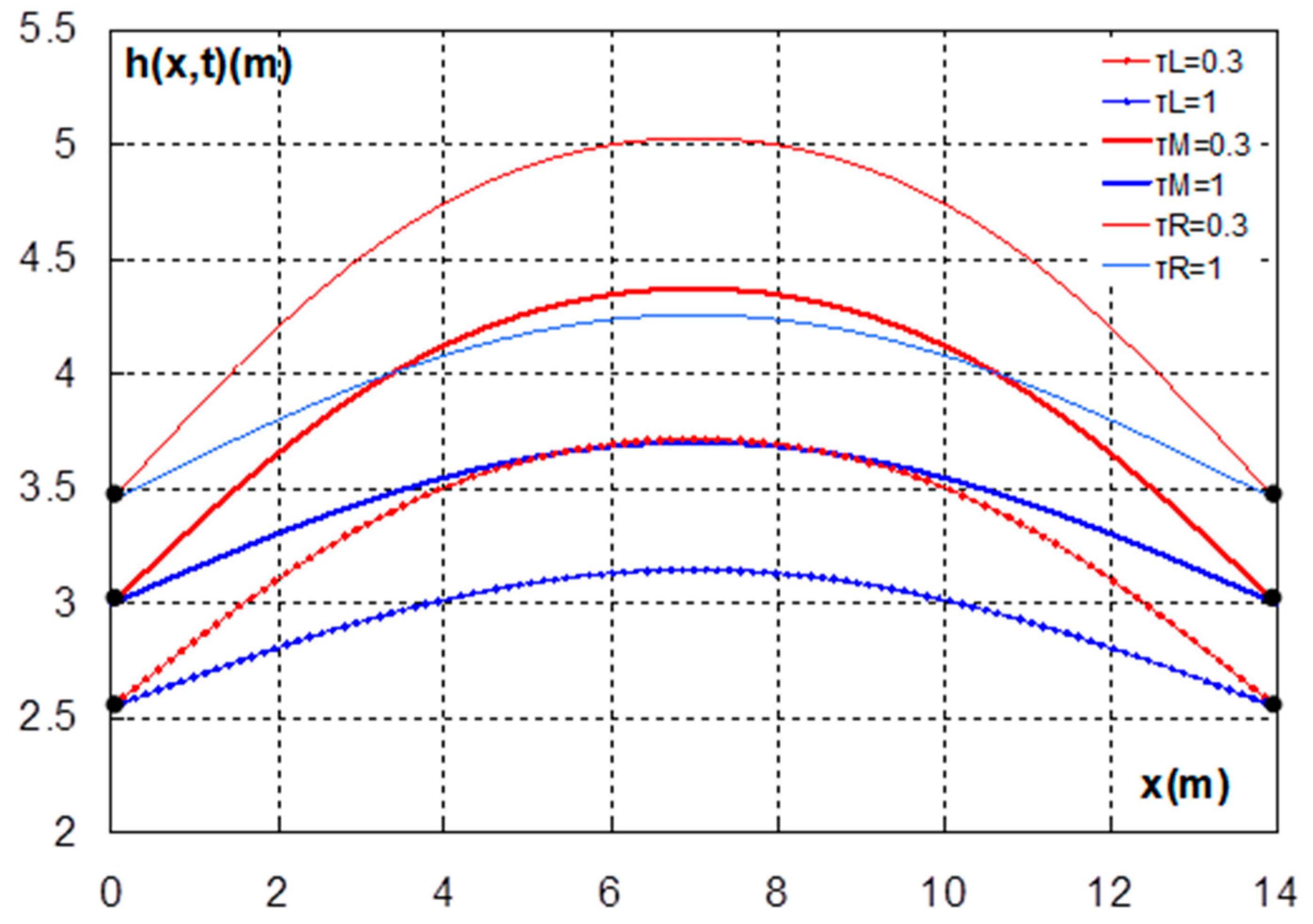
For the case of Figure 1, the following are valid: Κ = 0.2 m/d, S = 0.2, d = 3 m, E = 4.5 m, and α1 = KB/S = 3.75 m2/d. An uncertainty of 15% is introduced to the boundary and initial flow conditions. Based on the above, the values are calculated and plotted on Figure 3, Figure 4, Figure 5, Figure 6, Figure 7 and Figure 8. Specifically, in Figure 3, the fuzzy boundary and initial flow conditions are presented while Figure 4 presents the drain water table profiles for the non-dimensional times of τ = 0.3 and τ = 1.
Figure 5 provides the water table membership functions for the non-dimensional times of τ = 0.3 and τ = 1 at the position x = 3.5 m. From this figure, the results indicate that at the position x = 3.5 m and for τ = 1, for the classical case, the h drain value is equal to 3.49 m. On the other hand, based on fuzzy logic and also on the possibility theory, for α = 0.05, the above value is in the interval [2.99, 3.99] with a 95% degree of confidence.
Similarly, Figure 6 shows the membership function of the water table for the non-dimensional times of τ = 0.3 and τ = 1 at the position x = 7 m. From this figure, the results indicate that at the position x = 7 m and for τ = 1, for the classical case, the h drain value is equal to 3.7 m. On the other hand, based on fuzzy logic and also on the possibility theory, for α = 0.05, the above value is in the interval [3.17, 4.23] with a 95% degree of confidence.
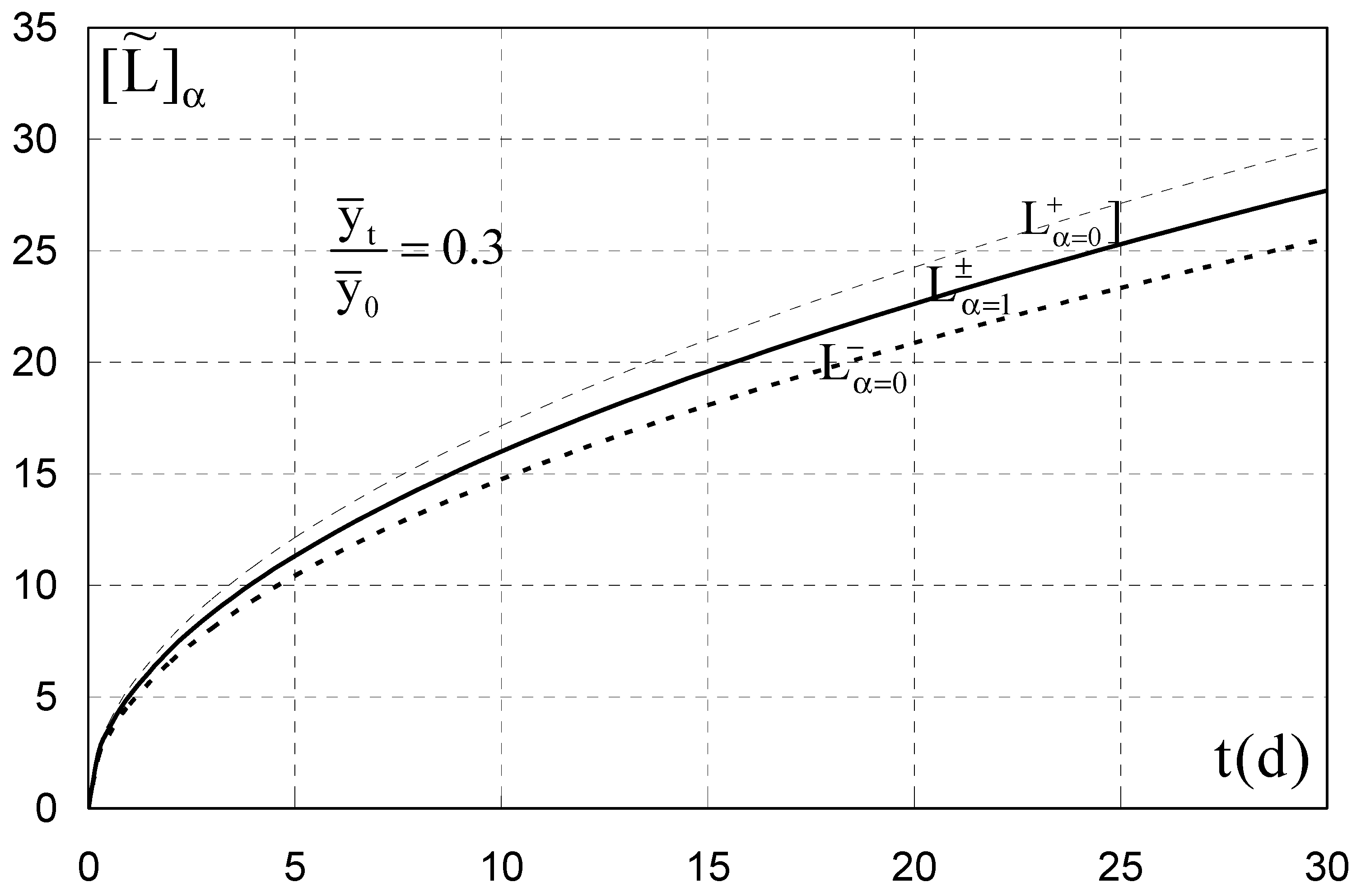
Figure 7 presents the drain spacing membership functions for τ = 0.3. Finally, Figure 8 shows the variation of the drain spacing for the above values (K, B, S, etc.) with respect to time, in days. From Figure 7 and Figure 8 and based on the above values, for the non-dimensional time τ = 0.3(t = 1.83d), results indicate that in classical logic the drain spacing value is Lc = 15 m. However, based on the fuzzy logic and also on the possibility theory for α = 0.05, the value of drain spacing is in the interval L = [13.89, 16.03] with a 95% degree of confidence.
6. Discussion and Future Research
Well-drained agricultural lands have longer periods with good soil health, and this could lead to a more efficient production as well as economic benefits. To find the optimal drain spacing is very crucial in order to design a drainage system, and it is still a tedious task. Farmers, landowners, agri-consultants and contractors are some cases that are directly interested in the accurate drain spacing.
Based on our expertise in these fields we believe that the most crucial uncertainties of this drainage problem appear on the boundary and initial flow conditions; in addition, previous works have dealt with these uncertainties in groundwater flow problems [41,42,43,44]. These uncertainties could have bad consequences for the soils and the plant growth if they are not included in the calculations. In this context, the innovative findings of this research regarding the drain spacing calculation, could strongly support the general land reclamation problem and therefore international and European directives such as the Common Agricultural Policy (CAP) and the Sustainable Development Goals (SDGs).
We must also mention that drainage no longer plays the significant role in the food production process that it played in the previous years. However, it will continue to play a major part in maintaining the present levels of food production. This is valid especially of rainfed lands, much of whose productivity would diminish substantially without drainage, and particularly of irrigated land. Without drainage, a large part of the irrigated land in the arid and sub-arid zones would not be sustainable and would be doomed to degrade into a waterlogged and/or salinized wasteland. In addition, in the same context, our approach aims to prevent the inflow of water, due to the increase in the phreatic level of the aquifer, towards the aeration zone. The use of our approach in the future, for a drainage network design and construction, requires the knowledge of the intensity of the artificial rain coming from the irrigation, in order to accurately calculate the required remaining time of the useful water in the aeration zone needed by the root substrate for the plants to grow.
Our proposed solution could not be calibrated and validated at this phase, mainly due to the lack of in situ measurements of the various soil and hydraulic parameters. Our approach at the moment is in a theoretical framework but without affecting the accuracy and reliability of the solution, as this approach is based mainly on the well-known and tested Glover-Dumm equation by adding the uncertainty part. An extended version of this work could be undoubtably, and its validation with in-situ measurements under controlled conditions and field work, as well as its practical application in the field with possible comparisons with other fuzzy solutions of drain spacing, will probably be developed in the future.
Furthermore, it is crucial to highlight that the hydraulic conductivity and soil texture are key factors in determining the optimal drain spacing. Hydraulic conductivity is a soil parameter which demands in situ measurements such as the auger method or soil sample analysis in the laboratory; in addition, it is a parameter that presents great variability even at parcel levels, creating difficult conditions for its determination and costly laboratory and in situ analyses. However, its importance in the drain spacing equations is more than critical and future research could focus on the inclusion of the uncertainties contained in this parameter. In addition, and in this context, innovative low cost in situ solutions (such as a portable spectrometer) [45] could be used to measure key soil parameters and support the drain spacing problem with valuable input data.
7. Conclusions
The ADM theory allows for finding an approximate solution of the differential equations with a satisfactory accuracy and, in some cases, as in the present work, for the linearized Boussinesq equation, that is identical to the accurate analytical solution.
Based on Figure 4, Figure 5 and Figure 6, the results indicate that the absolute fuzzy value decreases when the time increases, while the relevant value remains the same. On the contrary, from Figure 8, which refers on the drain spacing, results indicate that the absolute fuzzy value increases when the time increases, while the relevant value again remains the same.
The Khastan and Nieto (2010) [36] and Bede and Stefanini theory (2013) [34] with the generalized Hukuhara (g-H) derivative, as well as its extension to the Allahviranloo et al. (2015) [35] partial differential equations, allows researchers to solve practical problems that are useful in engineering. It is now possible for engineers to take the fuzziness of the various sizes involved into consideration and to solve the fuzzy problems.
The importance of the possibility theory is very crucial because it allows the researchers to find, with a small risk, the interval of variation of the unknown variable value with a degree of confidence greater than 95%.
In our analysis, the climatic conditions were not actively considered as they are not strongly affecting the approach to construct the final proposed fuzzy analytical solution, which was the main goal of this work. All efforts focused on the scientific analysis and evaluation of the construction of the analytical solution by using the innovative Adomian decomposition method (see Appendix A). A general note is that this fuzzy approach is based on the Glover-Dumm equation which, until today, does not have any serious constraint regarding its implementation in different climatic zones. Thus, our approach could be implemented in all types of climatic zones around the globe.
Finally, it should be mentioned that the inclusion of the uncertainties in the hydraulic conductivity parameter combined with the boundary and initial flow condition uncertainties, are in the authors’ future plans, where the achievement could create a promising fuzzy melioration methodology related to the drain spacing problem.
Author Contributions
Conceptualization, C.T.; methodology, C.T. and N.S.; software, C.E., writing—original draft preparation, C.T. and N.S.; writing—review and editing, C.T., N.S. and K.P.; visualization, K.P. and C.E. All authors have read and agreed to the published version of the manuscript.
Funding
This research received no external funding.
Data Availability Statement
All data are enclosed in the manuscript.
Conflicts of Interest
The authors declare no conflict of interest.
Appendix A
This appendix describes the Adomian decomposition method (ADM). The authors consider it useful to provide an explanation of the method, as the proposed findings of this work are based on this method. For this reason, the ADM is described in brief.
Assume the following partial differential equation:
where represents a nonlinear differential operator involving linear and nonlinear terms. The linear terms are analyzed into L + R, where L is invertible, and R is the remaining linear operator. Usually, L is taken as an operator that avoids difficult integrations that arise when there are implicit functions. The above equation is written as follows:
where represents the nonlinear terms.
Now, we solve the equation with respect to :
Because L is invertible, we multiply both terms by L−1 and we have:
If it is an initial value problem, then an integral operator is considered as a definite integral from t0 to t. If, for example, L is an operator of 1st order, we will have that . Thus, the above equation is written:
According to Adomian (1988), the function u could be analyzed by the series with , while the nonlinear term could be analyzed by the series , in which the are called Adomian polynomials. Thus, the above expression can take the following form:
Therefore, the following are stated:
Adomian polynomials are formed for each nonlinear term and, actually, the A0 depends only on u0, A1 depends only on u0 and u1, A2 depends only on u0, u1 and u2, etc. All components of u are calculated and If the series converges, then the n-th partial term will be the approximate solution because by definition.
Many researchers have worked to find simple formulas for Adomian polynomials. Among them [24], a simple method was developed for the easy determination of polynomials and [25] a new simplifying algorithm was developed for computing polynomials. Therefore, according to [25], the nonlinear function is equal to: and the parametric expression of is: where λ is a parameter. Therefore, the equation will be:
The Adomian function results, if we take the n-order derivative in different members of the above expressions in terms of λ and set λ = 0:
References
- Ziccarelli, M.; Valore, C. Hydraulic conductivity and strength of pervious concrete for deep trench drains. Geomech. Energy Environ. 2018, 18, 41–55. [Google Scholar] [CrossRef]
- Qian, Y.; Zhu, Y.; Ye, M.; Huang, J.; Wu, J. Experiment and numerical simulation for designing layout parameters of subsurface drainage pipes in arid agricultural areas. Agric. Water Manag. 2021, 243, 106–455. [Google Scholar] [CrossRef]
- Karamouzis, D.; Zissis, T.; Terzidis, G. Non-dimensional Diagrams for Unsteady Drainage Problems with or Without recharge. Agric. Water Manag. 1988, 13, 145–156. [Google Scholar] [CrossRef]
- Hooghoudt, S.B. Bijdragen tot de Kennis van Enige Natuurkundige Grootheden van de Grond; Versl. Landbook Onderzoek; Algemeene Landsdrukkerij: The Hague, The Netherlands, 1940; Volume 46, pp. 515–707. [Google Scholar]
- Toksöz, S.; Kirkham, D. Steady Drainage of Layered Soils: II. Nomographs. J. Irrig. Drain. Div. 1971, 97, 1–37. [Google Scholar] [CrossRef]
- Ernst, L.F. Grondwaterstromingen in de Verzadigde Zone en Hun Berekening Bij Aanwezigheid van Horizontale Evenwijdige Open; Versl. Landbouwk. Onderz; Centrum voor Landbouwpublikaties en Landbouwdocumentatie: Wageningen, The Netherlands, 1962; Volume 76, p. 15. [Google Scholar]
- Terzides, G.; Karamouzis, D. Land Drainage; Ziti Ed.: Thessaloniki, Greece, 1986. (In Greek) [Google Scholar]
- Terzides, G. A simple and exact method for stratified drainage soils. In Proceedings of the 3rd National Conference EGME, Thessaloniki, Greece, October 2003. (In Greek). [Google Scholar]
- Tzimopoulos, C. Drainage Engineering-Well Hydrology; Ziti Ed.: Thessaloniki, Greece, 1982. (In Greek) [Google Scholar]
- Kirkham, D. Seepage of steady rainfall through soil into drains. Eos Trans. Am. Geophys. Union 1958, 39, 892–908. [Google Scholar] [CrossRef]
- Dagan, G. Steady Drainage of a Τwo-Layered Soil. J. Irrig. Drain. Div. 1965, 91, 51–64. [Google Scholar] [CrossRef]
- Van der Molen, W.H.; Wesseling, J. A solutiom in closed form and a series solution to replace the tables for the thickness of the equivalent layer in Hooghoudt’s drain spacing formula. Agric. Water Manag. 1991, 19, 1–16. [Google Scholar] [CrossRef]
- Ritzema, H.P. Subsurface Flow to Drains. In Drainage Principles and Applications; International Institute for Land Reclamation and Improvement: Wageningen, The Netherlands, 1994. [Google Scholar]
- Μishra, G.C.; Singh, V. A new drain spacing formula. Hydrol. Sci. J. 2007, 52, 338–351. [Google Scholar] [CrossRef] [Green Version]
- Afruzi, A.; Νazemi, A.H.; Sadraddini, A.A. Steady-state subsurface drainage of ponded fields by rectangular ditch drains. Irrig. Drain. 2014, 63, 668–681. [Google Scholar] [CrossRef]
- Dumm, L.D. Drain spacing formula. Agric. Eng. 1954, 35, 726–730. [Google Scholar]
- Dumm, L.D. Validity and use of the transient flow concept in subsurface drainage. In Proceedings of the ASAE Meeting, Memphis, TN, USA, 1 December 1960; pp. 4–7. [Google Scholar]
- Bureau of Reclamation. Drainage Manual; U.S. Department of the Interior: Washington, DC, USA, 1993.
- Tzimopoulos, C.; Terzidis, G. Écoulement non permanent dans un sol drainé par des fossés parallèles. J. Hydrol. 1975, 27, 73–93. [Google Scholar] [CrossRef]
- McDonald, M.G.; Harbaugh, A.W. A Modular Three-Dimensional Finite-Difference Ground-Water Flow Model; Techniques of Water-Resource Investigations of the United States Geological Survey, Book 6, Modeling Techniques; U.S. Geological Survey: Reston, VA, USA, 1988.
- Awad, A.; El-Rawy, M.; Abdalhi, M.; Al-Ansari, N. Evaluation of the DRAINMOD Model’s Performance Using Different Time Steps in Evapotranspiration Computations. Hydrology 2022, 9, 40. [Google Scholar] [CrossRef]
- Skaggs, R.W.; Youssef, M.A.; Chescheir, G.M. DRAINMOD: Model use, calibration and validation. Trans. ASABE Am. Soc. Agric. Biol. Eng. 2012, 55, 1509–1522. [Google Scholar] [CrossRef]
- Wrachien, D.D.; Mambretti, S. Irrigation and drainage systems in flood-prone areas: The role of mathematical models. Austin J. Irrig. 2015, 1, 1002. [Google Scholar]
- Zhang, J.; Huang, S.; Cheng, L.; Ai, S.; Teng, B.; Guan, Y.; Xue, Y. A mathematical model for drainage and desorption area analysis during shale gas production. J. Nat. Gas Sci. Eng. 2014, 21, 1032–1042. [Google Scholar] [CrossRef]
- Singh, A. Environmental problems of salinization and poor drainage in irrigated areas: Management through the mathematical models. J. Clean. Prod. 2019, 206, 572–579. [Google Scholar] [CrossRef]
- Mehdinejadiani, B.; Naseri, A.A.; Jafari, H.; Ghanbarzadeh, A.; Baleanu, D. A mathematical model for simulation of a water table profile between two parallel subsurface drains using fractional derivatives. Comput. Math. Appl. 2013, 66, 785–794. [Google Scholar] [CrossRef]
- Klir, G.J.; Bo, Y. Fuzzy Sets and Fuzzy Logic, Theory and Applications; Prentice Hall: Upper Saddle River, NJ, USA, 1995. [Google Scholar]
- Goguen, J.A. L-fuzzy sets. J. Math. Anal. Appl. 1967, 18, 145–174. [Google Scholar] [CrossRef] [Green Version]
- Adomian, G. A Review of the Decomposition Method in Applied Mathematics. J. Math. Anal. Appl. 1988, 135, 501–544. [Google Scholar] [CrossRef] [Green Version]
- Wazwaz, A.M. A new algorithm for calculating Adomian polynomials for nonlinear operators. Appl. Math. Comput. 2000, 111, 53–69. [Google Scholar]
- Zhu, Y.; Chang, Q.; Wu, S. A new algorithm for calculating Adomian polynomials. Appl. Math. Comput. 2005, 169, 402–416. [Google Scholar] [CrossRef]
- Zadeh, L.A. Fuzzy Sets. Inf. Control 1965, 8, 338–353. [Google Scholar] [CrossRef] [Green Version]
- Mak, M.K.; Leung, C.; Harko, T. A Brief Introduction to the Adomian Decomposition Method, with Applications in Astronomy and Astrophysics. arXiv 2021, arXiv:2102.10511. [Google Scholar]
- Bede, B.; Stefanini, L. Generalized differentiability of fuzzy-valued functions. Fuzzy Sets Syst. 2013, 230, 119–141. [Google Scholar] [CrossRef] [Green Version]
- Allahviranloo, T.; Gouyandeh, Z.; Armand, A.; Hasanoglu, A. On fuzzy solutions for heat equation based on generalized Hukuhara differentiability. Fuzzy Sets Syst. 2015, 265, 1–23. [Google Scholar] [CrossRef]
- Khastan, A.; Nieto, J.J. A boundary value problem for second order fuzzy differential equations. Nonlinear Anal. 2010, 72, 3583–3593. [Google Scholar] [CrossRef]
- Dubois, D.; Prade, H. Possibility theory, probability theory and multiple-valued logics: A clarification. Ann. Math. Artif. Intell. 2001, 32, 35–66. [Google Scholar] [CrossRef]
- Negoita, C.V.; Ralescu, D.A. Representation theorems for fuzzy concepts. Kybernetes 1975, 4, 169–174. [Google Scholar] [CrossRef]
- Goetschel, R.; Voxman, W. Elementary fuzzy calculus. Fuzzy Sets Syst. 1986, 18, 31–43. [Google Scholar] [CrossRef]
- Mondal, S.P.; Roy, T.K. Solution of second order linear differential equation in fuzzy Environment. Ann. Fuzzy Math. Inform. 2015, 10, 1–25. [Google Scholar]
- Tzimopoulos, C.; Papadopoulos, K.; Evangelides, C.; Papadopoulos, B. Fuzzy solution to the unconfined aquifer problem. Water 2019, 11, 54. [Google Scholar] [CrossRef] [Green Version]
- Tzimopoulos, C.; Papadopoulos, K.; Papadopoulos, B.; Samarinas, N.; Evangelides, C. Fuzzy solution of nonlinear Boussinesq equation. J. Hydroinformatics 2022, 24, 1127–1147. [Google Scholar] [CrossRef]
- Samarinas, N.; Tzimopoulos, C.; Evangelides, C. Fuzzy numerical solution to the unconfined aquifer problem under the Boussinesq equation. Water Supply 2021, 21, 3210–3224. [Google Scholar] [CrossRef]
- Samarinas, N.; Tzimopoulos, C.; Evangelides, C. An efficient method to solve the fuzzy Crank–Nicolson scheme with application to the groundwater flow problem. J. Hydroinformatics 2021, 24, 590–609. [Google Scholar] [CrossRef]
- Karyotis, K.; Angelopoulou, T.; Tziolas, N.; Palaiologou, E.; Samarinas, N.; Zalidis, G. Evaluation of a Micro-Electro Mechanical Systems Spectral Sensor for Soil Properties Estimation. Land 2021, 10, 63. [Google Scholar] [CrossRef]
Figure 1.
Drains with distance d(m) from the impermeable layer.

Figure 2.
The straight line E = 3 in the form of the Fouries series.

Figure 3.
Profile of the free surface for the non-dimensional times of τ = 0.3 and τ = 1 (where τL indicates the left part of the α-cut, tR the right part and tM for α = 1).
Figure 3.
Profile of the free surface for the non-dimensional times of τ = 0.3 and τ = 1 (where τL indicates the left part of the α-cut, tR the right part and tM for α = 1).

Figure 4.
Membership functions for the boundary and initial flow conditions: ().
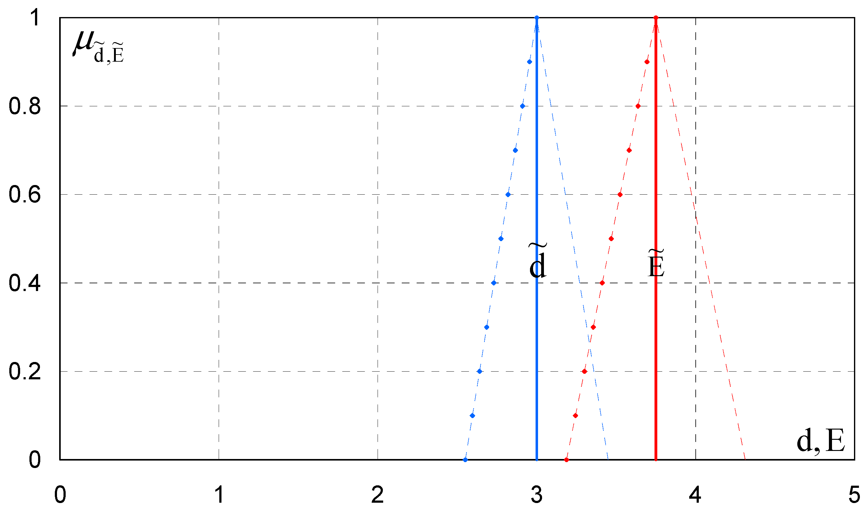
Figure 5.
Membership functions of the free surface flow at h(x,t) at the position xm = 3.50 m.
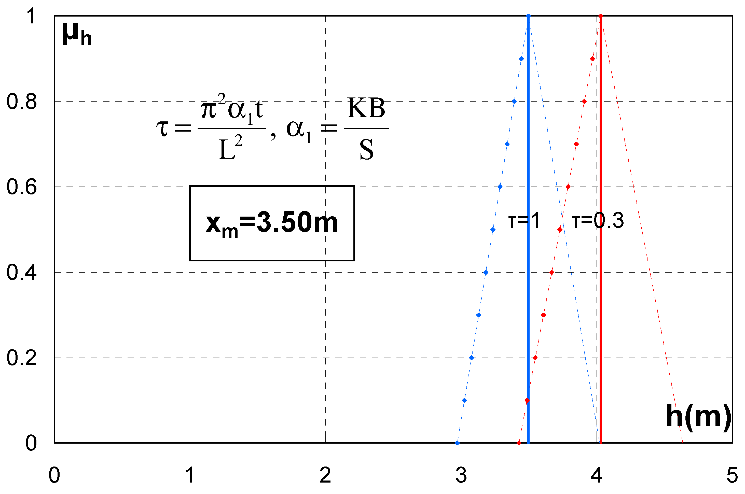
Figure 6.
Membership functions of the free surface flow at h(x,t) at the position xm = 7.00 m.

Figure 7.
Membership function for the drain spacing.
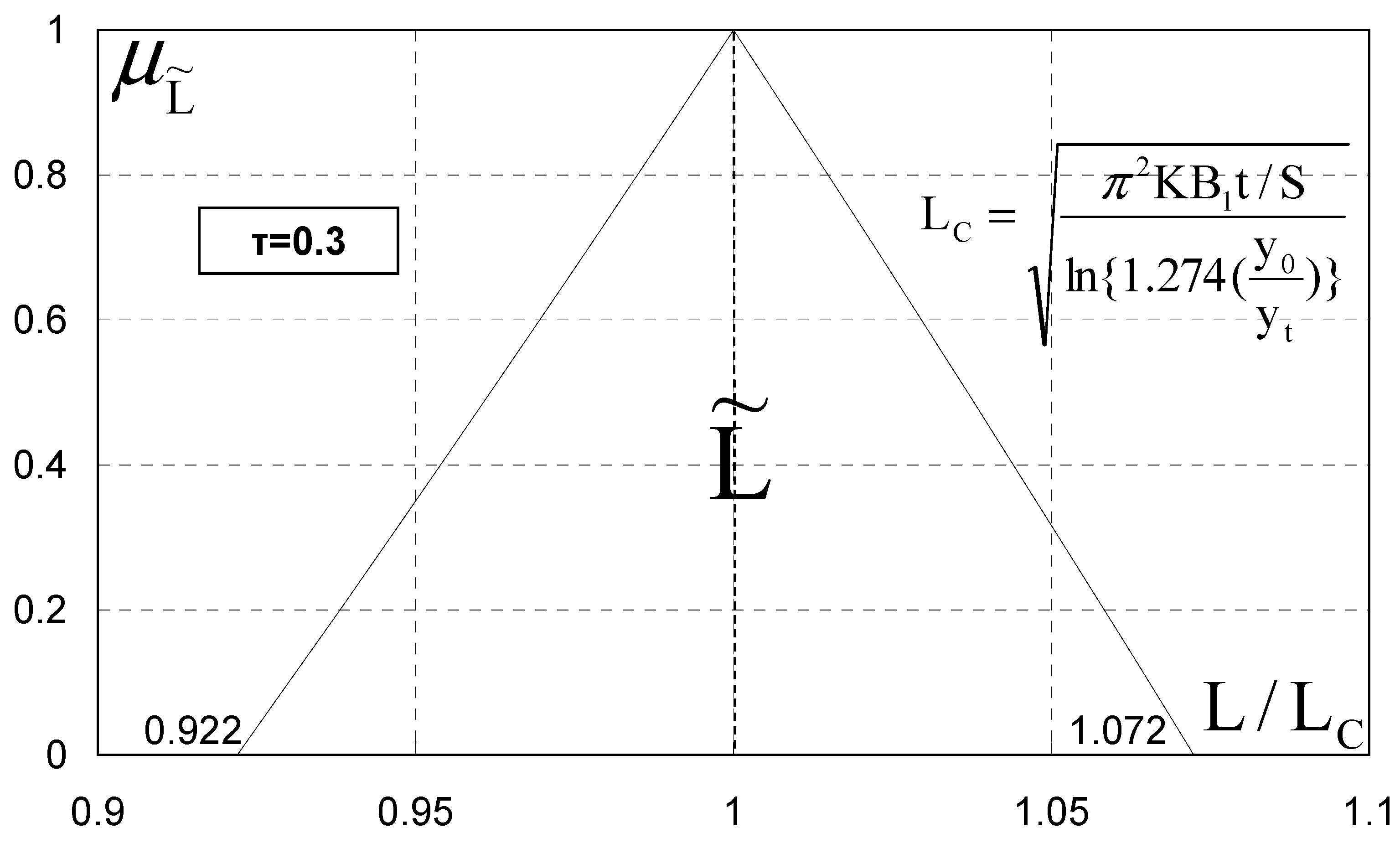
Figure 8.
Fuzzy drain spacing with respect to time for .
Disclaimer/Publisher’s Note: The statements, opinions and data contained in all publications are solely those of the individual author(s) and contributor(s) and not of MDPI and/or the editor(s). MDPI and/or the editor(s) disclaim responsibility for any injury to people or property resulting from any ideas, methods, instructions or products referred to in the content. |
© 2023 by the authors. Licensee MDPI, Basel, Switzerland. This article is an open access article distributed under the terms and conditions of the Creative Commons Attribution (CC BY) license (https://creativecommons.org/licenses/by/4.0/).
Share and Cite
MDPI and ACS Style
Tzimopoulos, C.; Samarinas, N.; Papadopoulos, K.; Evangelides, C. Fuzzy Unsteady-State Drainage Solution for Land Reclamation. Hydrology 2023, 10, 34. https://doi.org/10.3390/hydrology10020034
AMA Style
Tzimopoulos C, Samarinas N, Papadopoulos K, Evangelides C. Fuzzy Unsteady-State Drainage Solution for Land Reclamation. Hydrology. 2023; 10(2):34. https://doi.org/10.3390/hydrology10020034
Chicago/Turabian StyleTzimopoulos, Christos, Nikiforos Samarinas, Kyriakos Papadopoulos, and Christos Evangelides. 2023. "Fuzzy Unsteady-State Drainage Solution for Land Reclamation" Hydrology 10, no. 2: 34. https://doi.org/10.3390/hydrology10020034
Note that from the first issue of 2016, this journal uses article numbers instead of page numbers. See further details here.