ANN-Based Predictors of ASR Well Recovery Effectiveness in Unconfined Aquifers

Abstract

In this study, we present artificial neural networks (ANNs) to aid in a reconnaissance evaluation of an aquifer storage and recovery (ASR) well. Recovery effectiveness (REN) is the proportion of ASR-injected water recovered during subsequent extraction from the same well. ANN-based predictors allow rapid REN prediction without requiring preparation for and execution of solute transport simulations. REN helps estimate blended water quality resulting from a conservative solute in an aquifer, extraction for environmental protection, and other uses, respectively. Assume that into an isotropic homogenous portion of an unconfined, one-layer aquifer, extra surface water is injected at a steady rate during two wet months (61 days) through a fully penetrating ASR well. And then, water is extracted from the well at the same steady rate during three dry months (91-day period of high demand). The presented dimensionless input parameters were designed to be calibrated within the ANNs to match REN values. The values result from groundwater flow and solute transport simulations for ranges of impact factors of unconfined aquifers. The ANNs calibrated the weighting coefficients associated with the input parameters to predict the achievable REN of an ASR well. The ASR steadily injects extra surface water during periods of water availability and, subsequently, steadily extracts groundwater for use. The total extraction volume equaled the total injection volume at the end of extraction day 61. Subsequently, continuing extraction presumes a pre-existing groundwater right.

1. Introduction

1.1. Recovery Effectiveness (REN) of Aquifer Storage and Recovery (ASR) Well

The application of water resources management to increase water sustainability involves controlling water movement to (a) increase beneficial use and (b) avoid damage to life and nature. The managed aquifer recharge (MAR) method helps achieve long-term water sustainability by using available stormwater runoff, treated wastewater, or other surface water [1]. As a relatively inexpensive way to improve water supply, one of the MAR tools that injects water into an aquifer is aquifer storage and recovery (ASR) wells. The wells are especially useful where there is limited space, high population density, and increasing demand for groundwater [2,3]. ASR is a tool for integrating surface water and groundwater. It can help provide water storage in regions that have periods of both drought and intense precipitation [4]. ASR involves storing available excess surface water within an aquifer and subsequently recovering the water when advantageous. Note, ASR systems’ fundamental concept and structure design are based on one vertical well for injection and extraction. Another MAR tool, ASTR (Aquifer Storage Transfer and Recovery) system, uses one vertical well for injection and another one in a different location for extraction.

If available, extra surface water is injected into an aquifer via an ASR well. After the availability of surface water for injection ceases, the same ASR well immediately begins extracting groundwater for irrigation use. REN represents the proportion of injected water molecules contained within ASR extracted water. REN cannot exceed a value of one.

REN differs in recovery efficiency (RE) used to quantify the performance of ASR wells. The wells inject water into brackish, saline, or coastal aquifers and extract blended water that does not need treatment before its intended use [5,6]. RE can exceed a value of one as it is the ratio of the extracted volume that does not need treatment to the injectate volume [7,8,9,10,11,12,13].

REN is important in situations requiring knowledge of how much of the injected water is subsequently extracted or how much remains in the aquifer. Sometimes, modest mixing of (un)treated surface water or stormwater with groundwater in an aquifer is legally and environmentally acceptable. Predicting REN helps estimate the degree of blending that will occur. Forghani and Peralta [14] used a counting molecule method to predict the effectiveness (REN) of ASR well recovery instead of assessing the escape of injectate. The relation between REN and RE is:

$$\mathrm{R}\mathrm{E}=\mathrm{R}\mathrm{E}\mathrm{N}\left({\mathrm{V}}_{\mathrm{E}}\right)+\frac{\mathrm{V}(\mathrm{E},\mathrm{a}\mathrm{m}\mathrm{b})}{{\mathrm{V}}_{\mathrm{i}\mathrm{n}\mathrm{j}}}$$

(1)

where $\mathrm{V}\left(\mathrm{E},\mathrm{a}\mathrm{m}\mathrm{b}\right)$ is the volume of ambient groundwater in the extracted water, V_E is the total volume of extracted water, and V_inj is the total volume of injectate.

Situations in which injected water and native groundwater have similar quality are particularly challenging for predicting REN in the field. Field tracer tests have been performed to predict injectate recovery [15,16,17] but involve much uncertainty [18].

Thus, a simplified procedure or tool is needed to predict REN for ASR operations in unconfined aquifers, which are nonlinear systems. In recent years, a type of artificial intelligence (AI), artificial neural network (ANN), has been broadly used to predict groundwater quality and quantity [14,19,20,21]. Here, the application of this AI type helps quantify injectate recovery (REN) for ASR systems in unconfined aquifers.

1.2. Application of Artificial Neural Network (ANN)

An artificial neural network (ANN) simplifies biological neural networks to simulate human cognitive abilities via a mathematical structure [22]. ANN can develop theoretical or empirical relationships between input(s) and output(s) data to model nonlinear water resource systems [23,24]. This tool is used in hydrology, hydraulics, and water resources management for various tasks, such as forecasting water and groundwater levels and quality, modeling sediment, estimating rainfall–runoff, and managing floods [20]. The drawbacks of ANN [25] involve defining the optimal network structure and training its parameters. Thus, optimization algorithms are necessary to discover global and optimal solutions within complex parameter spaces. The algorithms help mitigate overparameterization and ensure error minimization. But it is important to note that achieving a low training error does not always guarantee good performance [25].

As published studies have shown, the calibration of different ANN models can be used to simulate and forecast water table fluctuations. Such models improve water supply planning in areas where aquifer information is not available [26,27,28]. In Taiwan, backpropagation of ANN forecasted the variation in groundwater quality resulting from seawater salinization and arsenic pollutant factors [29]. For predicting iodine levels of groundwater in China, an ANN was developed to aid environmental management because traditional analytical techniques are time consuming, difficult, and expensive [30]. Banerjee et al. [31] calibrated ANN to present a simpler and more accurate alternative to SUTRA (Saturated–Unsaturated Transport) numerical model techniques for groundwater salinity prediction. In general, understanding ANN structure and operation and nonlinear hydrologic processes is crucial for modeling rainfall–runoff, streamflow, groundwater management, water quality simulation, and precipitation [32].

For ASR operation within confined freshwater aquifers, ANN development predicts REN, and is an alternative to solute transport numerical simulation [14]. The present study tackles injectate-recovery (REN) prediction of ASR for specific times within unconfined aquifers and uses the ANN tool for the prediction in such nonlinear systems.

1.3. ANN Structure

An ANN structure to predict responses of nonlinear systems includes components such as: (a) input(s); (b) neuron(s) involving different numbers and arrangements; (c) output(s); and (d) a transfer (activation) function to interconnect the input parameters and neuron(s) to output(s). Figure 1 shows three layers (minimum number of layers) illustrating the positions of the ANN components: (a) the input layer; (b) one hidden layer; and (c) the output layer. In the layers, they are n inputs (I1 to In), n neurons (N1 to Nn), and an output (O1), respectively (Figure 1).

Defining inputs within the input layer is based on their impacts on the output(s) for prediction of the output(s). For instance, Sahoo et al. [24] applied known and important input parameters relatively to predict pesticide occurrence in wells. Forghani and Peralta [14] utilized input parameters that impact REN prediction for confined freshwater aquifers.

In published studies, the optimum number of neurons in an ANN has been defined as less than the number of input parameters [33]. Notably, increasing the number of neurons in a hidden layer and the number of hidden layer(s) can result in (a) a significant nondecreasing in root mean square error (RMSE) [29] and (b) losing the generalization ability of the ANN prediction for a new data set [24,34,35]. Thus, finding the optimum number of neurons and hidden layers in an ANN structure involves multiple “trials and errors” [24].

In the position of the hidden layer, ANN uses a linear, non-linear, or logic transfer (activation) function that provides an output corresponding to a weighted summation of the input parameters [31,36]. Among various transfer functions, sigmoid function ($f\left(u\right)=\frac{1}{1+e^{-u}}$) is a typical function having values of responses from 0 to 1 for a range of input parameters [19,36].

In this study, the presented suite of ANN using values of dimensionless analytical parameters (terms) is a tool to predict REN for specific times. The ANN-based predictors assist in estimating the retrieval of injectate, which is not simply the inverse process of the injectate’s movement in the down gradient. Employed ranges of impact factor values exceed the ranges of values reported for a representative 756 km² (288 mi²) shallow unconfined aquifer in an intermountain valley in the U.S. Great Basin. Herein, the number of neurons and hidden layers for ANN are one and one, respectively. The numbers were discovered by using a trial-and-error method in reference to statistical analyses. In short, REN evaluation involves estimating solute concentrations within ASR-extracted water and solute remaining within the aquifer. Water users and environmental protection scientists are interested in both.

2. Materials and Methods

2.1. Parameters and Procedures for REN Simulation and Prediction

2.1.1. Overview

Section 2.1 provides an overview of assumptions, parameters, and procedures employed to derive REN values first via simulation and then prediction. It is assumedly desirable to increase groundwater availability during a dry period (June–August) by injecting available excess surface water into an unconfined aquifer during a preceding wet period (April–May). This section defines the factors that impact REN and identifies the ranges of impact factor values that exist in Salt Lake Valley, Utah.

After the selection of approximately half-month durations for flow and solute transport simulations, standard methods are used in estimating (a) the advective plume length after two months (61 days) of injection, (b) the longitudinal dispersivity, (c) the Courant number, (d) the maximum time step size, (e) the total number of simulation time steps, and (f) the time steps per each stress period. These estimates enable preparing a groundwater aquifer model domain sufficiently large that assumed injection and extraction rates will not appreciably affect any employed boundary conditions.

To cover the ranges of REN-affecting factors, 48,000 unique input files were prepared for flow and solute transport simulations that were then processed in parallel. From the simulation results, the procedure required computing a simulated REN response, identifying impact factor combinations, and developing an artificial neural network (ANN) for the REN prediction. The ANN uses values of dimensionless analytical terms containing the impact factors to obtain the ANN-associated weighting coefficient values for the prediction. Finally, a statistical comparison of simulated versus ANN-based predicted values of REN determined the accuracy of the ANN-based predictors.

2.1.2. Selection of REN Impact Factors and Their Value Ranges

Based upon work by Fetter [37], Bedient et al. [38], Pavelic et al. [11], Ward et al. [12,13], Bakker [5], Brown et al. [7], Smith et al. [4], and Forghani and Peralta [14], eight impact factors that affect REN are considered: (1) initial aquifer (background) hydraulic gradient; (2) horizontal hydraulic conductivity; (3) initial (original) aquifer saturated thickness; (4) porosity; (5) specific yield; (6) steady rates of injection and extraction; (7) durations of injection and extraction; and (8) well diameter. A total of 48,000 unique sets of impact factor data were obtained by applying the

Table 1. Impact factor value ranges.

Impact Factor	Range (SI)	Range (English)
Background hydraulic gradient	0.00001–0.015	0.00001–0.015
Horizontal hydraulic conductivity	4–20 (m/d)	13.124–65.61 (ft/d)
Initial aquifer saturated thickness	8–46 (m)	26.25–150.91 (ft)
Porosity	0.1–0.6	0.1–0.6
(Specific yield)/(porosity)	0.375–0.95	0.375–0.95
Specific yield	0.0375–0.57	0.0375–0.57
Daily constant injection rate *	5.451–327.06 (m3/d)	0.0022–0.132 (cfs) or 1–60 (gpm)
Well diameter	15.24 (cm)	6 (inch)

* Note, injection and extraction durations are two months (April and May) and three months (June, July, and August), respectively. Extraction begins when injection ceases.

value ranges for groundwater flow and solute transport simulations.

The ranges of background hydraulic gradient, horizontal hydraulic conductivity, and initial aquifer saturated thickness used here include the values employed for Layer 1 of a Salt Lake Valley groundwater model [39]. To set the 0.1–0.6 range of porosity values, this study also relies upon values from Gelhar et al. [40] and Heath [41]. To determine the specific yield range, the porosity range and a 0.375–0.95 range of ((specific yield)/porosity) quotients (Table 1) are used. The 5.451 to 327.06 m³/d (1 to 60 gpm) steady injection rate range approximates the range of one percent of the average local Red Butte Creek flow from 2014 through 2016 during April and May, which are the months of greatest streamflow [42]. The range of steady extraction rates is equal but opposite in sign to the injection rate range. The extraction duration is three months (Table 1).

2.1.3. Modeled System and Simulators

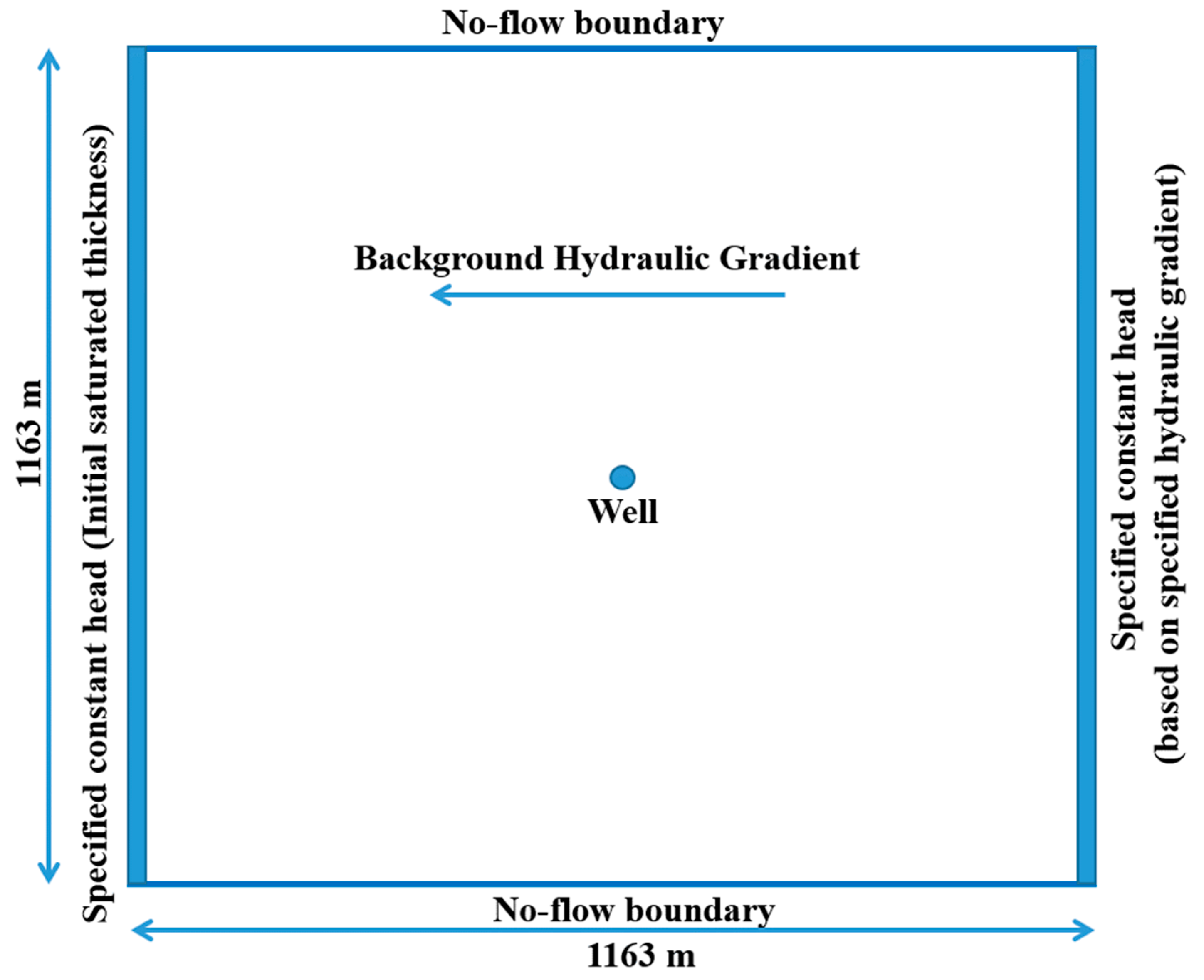
In essence, to allow computing REN with reasonable accuracy, the MODFLOW [43] finite difference flow model and its Multi-Node Well (MNW2) package and the MT3DMS solute transport model [44] are used. To distinguish the injectate from native groundwater and to provide a solute for transport simulation, a hypothetical 100 ppm concentration is assigned to the injectate. A fully penetrating ASR well in a homogenous, isotropic, freshwater, one-layer, unconfined aquifer is modeled, and extraction rates that are equal but opposite in sign to the injection rates are used. Specified constant-head boundaries on the eastern and western edges of a square model area, no-flow boundaries on the northern and southern edges, and the ASR well at the center are employed (Figure 2 and Figure 3).

Toward sizing the model and preparing model inputs, the greatest advective plume length that would occur by the end of the injection period for any set of Table 1 impact factor values is estimated. Ignoring gradient changes induced by an injection or groundwater mound, the greatest pore velocity would be 3 m/d (9.84 ft/d). After 61 days, this would yield a 183 m (600.4 ft) advective plume length. The assumed ground surface elevation of the model study area is a value of 100 m (328.08 ft). This results in (a) zero evapotranspiration loss of water from groundwater because the capillary fringe does not reach the overlying root zone. Note that the height of the capillary fringe in various soils does not exceed one meter [41] and (b) zero deep percolation into the same aquifer for this study. Because the unconfined aquifer includes a very thick initial saturated thickness, deep percolation might cause only a small relative change in transmissivity.

Longitudinal dispersion will lengthen the plume further. For an advective plume longer than one meter, the longitudinal dispersivity can be estimated as [40,45,46,47]:

$${\mathsf{\alpha }}_{\mathrm{L}}=0.83{\left[{\log }_{10}{\mathrm{L}}_{\mathrm{p}}\right]}^{2.414}$$

(2)

where α_L = longitudinal dispersivity (m) and ${\mathrm{L}}_{\mathrm{p}}$ = advective plume length (m). If ${\mathrm{L}}_{\mathrm{p}}\le 1\mathrm{m},{\mathsf{\alpha }}_{\mathrm{L}}=0.1{\mathrm{L}}_{\mathrm{p}}$.

MT3DMS uses the user-input Courant number (C) to control the advective process by decreasing oscillations, improving accuracy, and decreasing numerical dispersion. C = $(\mathrm{v}\times \Delta \mathrm{t})/\Delta \mathrm{x},$ where v = linear pore velocity, $\Delta \mathrm{x}$ = the grid cell dimension at the well location (0.5 m or 1.64 ft), and $\Delta \mathrm{t}$ is the maximum desirable time step size [48].

To determine the simulation time step size in days, suitable for the preferred spatial discretization, the grid Peclet number, P, as equaling 2C [48] is estimated. By assuming that P also equals ($\Delta \mathrm{x}/{\mathsf{\alpha }}_{\mathrm{L}})$, one can compute the maximum time step size desirable for use during injection.

The first estimation of the total number of time steps needed for the injection era was the integer result of dividing the total injection duration by the time step size. Those steps are partitioned equally into each injection stress period and then two more steps per period are added to increase the likelihood of successful simulation. All preliminary simulations for all data combinations used the same number of time steps for flow and solute transport simulations.

Preliminary simulations helped determine the horizontal domain size required to avoid appreciable boundary condition impact from groundwater pumping. Simulations employed the broadest extents of values of injection rate, extraction rate, horizontal hydraulic conductivity, initial (original) aquifer saturated thickness, and initial aquifer (background) hydraulic gradient. The resulting selected 1163 m by 1163 m (3815.62 ft. by 3815.62 ft.) model domain has 129 rows and 129 columns that transition smoothly from cell sizes of 10 m by 10 m (32.80 ft. by 32.80 ft.) to 0.5 m by 0.5 m (1.64 ft. by 1.64 ft.). In the center, the central smallest cell is a 7.62 cm (3 inch) radius vertical well. To have a uniform background hydraulic gradient and saturated thickness from the east to the west, the layer bottom elevation paralleled the desired initial water table.

MODFLOW2005 and MT3DMS simulations use 11 half-month stress periods to easily utilize available rainfall, streamflow, and plant water needs information. Period 1 simulates steady-state background heads. Transient periods 2–5 employ injection and periods 6–11 simulate extraction. Both models also use identical numbers of time steps per period, and that number can differ within a period. The MODFLOW2005 PCG solver uses a 0.01 m head change criterion and a 0.01 m residual convergence criterion. To simulate advection and dispersion, MT3DMS employs the total variation diminishing (TVD) package and the generalized conjugate gradient (GCG) solver. The injection stress period has varied time step durations. To avoid excessive processing time, the extraction period has a single time step (using even 300 time steps for extraction increases REN by less than 0.005).

From the impact factor value ranges in Table 1, five background hydraulic gradients, five hydraulic conductivities, eight injection or extraction rates, six porosity values, ten initial aquifer saturated thicknesses, and four (specific yield/porosity) ratios are used. For each of the 48,000 possible combinations, a different set of impact factor data for groundwater flow and solute transport simulations is prepared. As mentioned above, the 100 ppm of imaginary non-reactive solute (e.g., chloride or dissolved nitrate, etc.) is assigned to the injectate for distinguishing it from native groundwater. As commonly carried out in irrigation water management, chloride can be assumed to be a conservative contaminant. Freshwater, including rainwater, can dissolve halite in soil while recharging or passing through an aquifer. Also, under oxidizing conditions, dissolved nitrate is considered to be nonreactive and conservative [49]. Thus, in MTDMS flow and transport simulations in this study, the only simulated MT3DMS flow and transport simulations are advection and dispersion [40]. MT3DMS simulations provide both the mass of solute injected into the ASR well and the mass of solute recovered from the well. REN equals the extracted solute mass divided by the injected solute mass.

Because the processing time of a single MODFLOW2005-MT3DMS simulation might exceed an hour, parallel processing was used to drastically reduce the computing time [14,50,51]. The Message Passing Interface (MPI) [52,53,54] of the C++ programming language was utilized to implement parallel processing on multi-cored personal computers and on node clusters of the Center for High Performance Computing (CHPC) at the University of Utah, USA. About 47,000 of the 48,000 attempted MODFLOW2005-MT3DMS simulations were completed successfully. Each successful simulation provided the total mass of solute injected through the ASR well and the mass of solute recovered from the well. REN values were computed after 15, 30, 45, 61, 76, and 91 days of simulated extraction (REN15, REN30, REN45, REN61, REN76, and REN91, respectively).

2.2. Development and Evaluation of Dimensionless Analytical Parameters (Terms) for ANN-Based Predictors

2.2.1. Overview

This section describes the development of dimensionless analytical parameters (terms) as inputs for artificial neural networks (ANNs) that can rapidly predict REN values for use in lieu of numerical simulation models. Data employed for this section include the impact factors in Table 1 applied for the terms, resulting simulation outputs, and computed RENs. Section activities include (1) developing dimensionless analytical expressions that equal (a) a ratio of (extraction/plume) volumes, (b) a ratio of (capture zone/plume) widths, and (c) a ratio of (capture zone/plume) lengths; (2) developing artificial neural networks (ANNs) that apply the dimensionless analytical terms to predict REN values; and (3) defining statistical indices to evaluate ANN-based predictors. The first analytical expression (dimensionless volume) addresses a dimensionless volumetric ratio of the pumped volume that contains the plume volume at a specific time. Some initial trial and error tests for REN prediction were started using the dimensionless volume in regression processes. Regarding the results, it was concluded that the volume presents significant responses for REN prediction but is not sufficient. Also, logically hydraulic down gradient results in moving the plume from the ASR well location. Besides the dimensionless volume, the down-gradient width and length ratios were applied in ANN to modify how much of the plume volume was within the down-gradient capture zone for REN prediction. In the width and length ratios, a natural logarithm was applied to aid their non-linear magnitudes to be valued linearly for the prediction.

2.2.2. Development of Dimensionless Analytical Parameters (Terms)

The impact factors in Table 1 affect REN both in the field and as simulated using MODFLOW2005-MT3DMS. Some initial attempts for REN prediction were started using the impact factors as independent inputs within different artificial neural network (ANN) structures. However, these attempts did not meet the convergence criteria to predict REN. Then, dimensionless analytical terms were designed to be used by ANNs toward predicting dimensionless REN from simulation results. The terms consist of (a) a ratio of the volume of extracted water divided by the injectate plume volume at the time that extraction begins; (b) a natural logarithm of the ratio of the steady-state down-gradient capture zone width divided by the plume width at the end of the injection; and (c) a natural logarithm of the ratio of the steady-state down-gradient capture zone length divided by the advective plume length down-gradient at the end of the injection.

The volume of extracted water at a moment in time equals the extraction duration to that moment times the extraction rate. The volume of the injectate plume equals its 2D area times a representative vertical thickness. The area,${\mathrm{A}}_{\mathrm{p}}$, of an elliptical injection plume having a normal or Gaussian concentration distribution, a length of $3{\mathsf{\sigma }}_{\mathrm{x}}$, and a width of $3{\mathsf{\sigma }}_{\mathrm{y}}$, is:

$${\mathrm{A}}_{\mathrm{p}}=\mathsf{\pi }3{\mathsf{\sigma }}_{\mathrm{x}}3{\mathsf{\sigma }}_{\mathrm{y}}$$

(3)

where ${\mathsf{\sigma }}_{\mathrm{x}}$ is the standard deviation of concentration in the x direction, (L) $=\sqrt{2{\mathrm{D}}_{\mathrm{L}}\mathrm{t}};$ ${\mathsf{\sigma }}_{\mathrm{y}}$ is similarly defined; D_L and D_T are longitudinal and horizontal transverse dispersions (L²/T) that respectively equal ${\mathsf{\alpha }}_{\mathrm{L}}\times {\mathrm{v}}_{\mathrm{x}}$ and ${\mathsf{\alpha }}_{\mathrm{T}}\times {\mathrm{v}}_{\mathrm{y}}$; α_L and α_T are horizontal longitudinal dispersivity and transverse dispersivity (L), respectively; v_x and v_y are the linear pore velocities in the longitudinal x and transverse y directions (L/T), respectively; and t is the injection duration (T) [37,38,55].

In the field, horizontal transverse dispersivity is typically an order of magnitude smaller than longitudinal dispersivity [40,44]. Freeze and Cherry [56] indicated that the above equations can be used for preliminary estimation of solute migration arising from small contaminant spills in simple hydrogeologic settings. Assuming the horizontal transverse dispersivity is one-tenth of the longitudinal dispersivity, by substitution, the plume area is:

$${\mathrm{A}}_{\mathrm{p}}=\mathsf{\pi }18\sqrt{0.1}{\mathsf{\alpha }}_{\mathrm{L}}\mathrm{v}\mathrm{t}$$

(4)

where v = the linear pore velocity.

An estimate of the 61-day plume volume is the sum of the volumes of a cylinder and a cone (the cylinder and cone represent the initial or original aquifer saturated thickness and injection or groundwater mound height, respectively). The cylinder volume equals the product of the plume area and the initial (original) aquifer saturated thickness (b_ist). The cone (injection or groundwater mound) volume equals the plume area times b_im/3. Thus, the plume volume is:

$${\mathrm{V}}_{\mathrm{p}}={\mathrm{A}}_{\mathrm{p}}\left({\mathrm{b}}_{\mathrm{i}\mathrm{s}\mathrm{t}}+{\frac{1}{3}\mathrm{b}}_{\mathrm{i}\mathrm{m}}\right)=\left(\mathsf{\pi }18\sqrt{0.1}{\mathsf{\alpha }}_{\mathrm{L}}\mathrm{v}\mathrm{t}\right)\times \left({\mathrm{b}}_{\mathrm{i}\mathrm{s}\mathrm{t}}+{\frac{1}{3}\mathrm{b}}_{\mathrm{i}\mathrm{m}}\right)$$

(5)

where V_p is the plume volume, b_ist is the initial (original) aquifer saturated thickness, and b_im is the MODFLOW2005 injection or groundwater mound height that is water above the initial water table. For about 48,000 combinations of the impact factor values in Table 1, this study determined injection or groundwater mound heights by MODFLOW2005 simulation of the unconfined aquifer.

Herein, employing a two-step equation-based process with a regression equation in Appendix A to estimate the b_im avoids the need to run MODFLOW2005 for new combinations of aquifer conditions.

Equation (6) shows the definition of a dimensionless volume (DLV) as the ratio of the volume of the extracted water (V_ext) and the plume volume (V_p):

$$\mathrm{D}\mathrm{L}\mathrm{V}=\frac{{\mathrm{V}}_{\mathrm{e}\mathrm{x}\mathrm{t}}}{{\mathrm{V}}_{\mathrm{p}}}$$

(6)

where V_ext = Q × t; Q = pumping extraction rate; and t = extraction duration.

Because after any duration of extraction REN is a) a cumulative and nonlinear relative mass and b) between 0 and 1, concerning these REN properties, term 1 includes the sigmoid function (an S-shaped nonlinear function with a response between 0 and 1) of the DLV:

$$\mathrm{T}\mathrm{e}\mathrm{r}\mathrm{m}1=\frac{1}{1+{\mathrm{e}}^{-\mathrm{D}\mathrm{L}\mathrm{V}}}$$

(7)

By substituting Equations (5) and (6):

$$\mathrm{T}\mathrm{e}\mathrm{r}\mathrm{m}1=\left[\frac{1}{1+{\mathrm{e}}^{-\frac{{\mathrm{V}}_{\mathrm{e}\mathrm{x}\mathrm{t}}}{{\mathrm{A}}_{\mathrm{p}}\left({\mathrm{b}}_{\mathrm{i}\mathrm{s}\mathrm{t}}+\frac{1}{3}{\mathrm{b}}_{\mathrm{i}\mathrm{m}}\right)}}}\right]$$

(8)

Term 2 is a natural logarithm of the ratio of the (steady-state down-gradient capture zone width)/(plume width at end of injection that is${3\mathsf{\sigma }}_{\mathrm{y}}$) in Equation (9). The steady-state down-gradient capture zone width equals $\{\mathrm{Q}/(4\mathrm{K}{\mathrm{b}}_{\mathrm{i}\mathrm{s}\mathrm{t}}\mathrm{i}\left)\right\}$ [57]. The plume width (${3\mathsf{\sigma }}_{\mathrm{y}}$) is defined for Equation (3):

$$\mathrm{T}\mathrm{e}\mathrm{r}\mathrm{m}2=\mathrm{L}\mathrm{N}\left(\frac{\frac{\mathrm{Q}}{4\mathrm{K}{\mathrm{b}}_{\mathrm{i}\mathrm{s}\mathrm{t}}\mathrm{i}}}{3\times \sqrt{2\times 0.1\times {\mathsf{\alpha }}_{\mathrm{L}}\times \mathrm{v}\times {\mathrm{t}}_{\mathrm{i}\mathrm{n}\mathrm{j}}}}\right)$$

(9)

where LN is the natural logarithm; Q is the pumping extraction rate (L³/T); K is the horizontal hydraulic conductivity (L/T); b_ist is the initial (original) aquifer saturated thickness (L); i is the initial aquifer (background) hydraulic gradient (-); α_L is the horizontal longitudinal dispersivity (L); v is the linear pore velocity (L/T); and t_inj is the injection duration, 61 days (T).

Term 3 is a natural logarithm of the ratio of the (steady-state down-gradient capture zone length)/(length of advective plume down-gradient at end of injection):

$$\mathrm{T}\mathrm{e}\mathrm{r}\mathrm{m}3=\mathrm{L}\mathrm{N}\left(\frac{\frac{\mathrm{Q}}{2\mathsf{\pi }\mathrm{K}{\mathrm{b}}_{\mathrm{i}\mathrm{s}\mathrm{t}}\mathrm{i}}}{\frac{\mathrm{K}\mathrm{i}{\mathrm{t}}_{\mathrm{i}\mathrm{n}\mathrm{j}}}{\mathrm{n}}}\right)$$

(10)

where LN is the natural logarithm; the steady-state down-gradient capture zone length is $\{\mathrm{Q}/(2\mathsf{\pi }\times \mathrm{K}\times {\mathrm{b}}_{\mathrm{i}\mathrm{s}\mathrm{t}}\times \mathrm{i}\left)\right\}$ [57]; Q is the pumping extraction rate (L³/T); π is 3.1416; K is the horizontal hydraulic conductivity (L/T); b_ist is the initial (original) aquifer saturated thickness (L) and the advective plume length down-gradient of the well at end of injection (L) is $\left\{\right(\mathrm{K}\mathrm{i}{\mathrm{t}}_{\mathrm{i}\mathrm{n}\mathrm{j}})/\mathrm{n}\}$; i is initial aquifer (background) hydraulic gradient; t_inj is the injection duration, 61 days (T); and n is porosity (-).

Therefore, by using values of such terms as inputs, artificial neural networks (ANNs) can predict injectate recovery (REN) for the specific times.

2.2.3. Development of ANN to Predict REN

As mentioned above, a presented artificial neural network (ANN) represents a mathematical relationship between the REN output and the dimensionless analytical terms computed for Table 1 ranges of impact factor values. In essence, each ANN uses the dimensionless ratios of volume, width, and length (respectively, terms 1–3) to predict REN for a specific extraction duration. Herein, ANN development employed the neuralnet package of the R software [36].

In advance, to find an optimal number of neurons, hidden layers, and outputs, the trial-and-error method was applied to execute preliminary runs of the ANN using (a) the impact factors as independent inputs within various ANN structures with different numbers of hidden layers, neurons, and one and multi-REN outputs and (b) the terms as inputs (note: the first term was defined via regression processes) within one ANN structure for predicting all six REN values. The properties of these runs were various numbers of (i) hidden layers and (ii) neurons of the hidden layers. In both sets of runs, the ANN could not meet the convergence criteria or predict REN accurately.

Thus, the presented ANN structure and properties for six REN values concerning accuracy and simplicity were defined (Figure 4) as follows: (a) three input values of terms 1, 2, and 3; (b) one output REN value for a specific time; (c) a network type of resilient backpropagation with weight backtracking; (d) a network threshold of 0.01 for training; (e) one network repetition for training; (f) one hidden layer; (g) one neuron in the hidden layer; (h) a logistic transfer (activation) function; (i) biases of 1 in input and hidden layers; and (j) a differentiable error function of “sum of squared errors”. And the rest of the properties used were from the neuralnet default.

The ANN structure in Figure 4 is named “feedforward” [58,59,60,61]; this structure transfers information from a previous layer to the next one. Here, all term 1–3 inputs and bias 1 connect to the neuron in the hidden layer that is linked to the output along with the hidden layer bias. The associated weighting coefficients represent the connection importance in the network. The value of the neuron in the hidden layer is calculated by using the sigmoid activation function on the sum of the products of the values of the bias, the terms (inputs), and their associated weights (Equation (11)).

$${\mathrm{N}}_1=\frac{1}{1+\mathrm{E}\mathrm{X}\mathrm{P}\left[-\left(1\times {\mathrm{W}}_{01}+\mathrm{T}\mathrm{e}\mathrm{r}\mathrm{m}1\times {\mathrm{W}}_{11}+\mathrm{T}\mathrm{e}\mathrm{r}\mathrm{m}2\times {\mathrm{W}}_{21}+\mathrm{T}\mathrm{e}\mathrm{r}\mathrm{m}3\times {\mathrm{W}}_{31}\right)\right]}$$

(11)

Then, the REN value is calculated by the sum of the bias value multiplied by its associated weighting value and products of the neuron value and the value of its associated weight (Equation (12)).

$$\mathrm{R}\mathrm{E}\mathrm{N}=\left(1\times {\mathrm{W}}_{01}^{\prime }\right)+\left({\mathrm{N}}_1\times {\mathrm{W}}_{11}^{\prime }\right)$$

(12)

Herein, six ANN algorithms sharing the same structure predict REN values for the six specific times (15, 30…, and 91 days after extraction) separately. For ANN calibration (training), the inputs (values of the terms 1 to 3) and the output (REN value for a specific time that is a result of MODFLOW2005-MT3DMS simulations) of the dataset were entered into the ANN model. The ANN model optimized the associated weighting values (W₀₁, W₁₁, W₂₁, W₃₁, W′₀₁, and W′₁₁) by minimizing the sum of squared errors that are differences between the simulated REN and the ANN-based predicted output (REN). For training the ANN, the whole dataset (the 47,000 MODFLOW2005-MT3DMS results or REN values) was split into 10 parts (named the 10-fold cross-validation method) randomly without replacement by applying a written code in R software (Figure 5). The 10-fold cross-validation method involves nine parts of the data set for training and one for testing or validation [58,60].

Based upon the cross-validation method and values of the following statistical indices (Figure A1), the best fold presented the six optimal values of the associated weighting coefficients (W₀₁, W₁₁, W₂₁, W₃₁, W′₀₁, and W′₁₁) for the ANN to predict REN for a specific time. In total, six ANN algorithms sharing the same structure provided 36 values of the associated weighting coefficients for six REN predictions (REN15, REN30…, and REN91). The required evaluation of the folds to select the optimal values of the weighting resulted in using some statistical indices that are presented in the following section.

2.2.4. Evaluation of Developed ANN-Based Predictors

The accuracy of the six ANN algorithms to predict six REN values was evaluated by applying statistical indices in

Table A1. Statistical indices.

Parameter	Formula *	Range	Applied by
Mean Error (ME)	$\frac{1}{\mathrm{n}}{\displaystyle \sum _{\mathrm{i}=1}^{\mathrm{n}}}\left({\mathrm{O}}_{\mathrm{i}}-{\mathrm{S}}_{\mathrm{i}}\right)$	−∞ < ME < +∞; Perfect: 0	Javan et al. [68]
Root Mean Square Error (RMSE)	$\sqrt{\frac{1}{\mathrm{n}}{\displaystyle \sum _{\mathrm{i}=1}^{\mathrm{n}}}{\left({\mathrm{O}}_{\mathrm{i}}-{\mathrm{S}}_{\mathrm{i}}\right)}^2}$	0 ≤ RMSE < +∞; Perfect: 0	Mentaschi et al. [69]; Javan et al. [68]; Jimeno-Sáez et al. [70]
Peak Weighted Root Mean Square Error (PWRMSE)	$\sqrt{\frac{1}{\mathrm{n}}{\displaystyle \sum _{\mathrm{i}=1}^{\mathrm{n}}}{\left({\mathrm{O}}_{\mathrm{i}}-{\mathrm{S}}_{\mathrm{i}}\right)}^2\times \left(\frac{{\mathrm{O}}_{\mathrm{i}}+\overline{\mathrm{O}}}{\overline{2\mathrm{O}}}\right)}$	0 ≤ PWRMSE < +∞; Perfect: 0	Javan et al. [68]
Pearson’s Correlation Coefficient (r)	$\frac{\sum _{\mathrm{i}=1}^{\mathrm{n}}\left({\mathrm{O}}_{\mathrm{i}}-\overline{\mathrm{O}}\right)\times \left({\mathrm{S}}_{\mathrm{i}}-\overline{\mathrm{S}}\right)}{\sqrt{\sum _{\mathrm{i}=1}^{\mathrm{n}}{\left({\mathrm{O}}_{\mathrm{i}}-\overline{\mathrm{O}}\right)}^2\times \sum _{\mathrm{i}=1}^{\mathrm{n}}{\left({\mathrm{S}}_{\mathrm{i}}-\overline{\mathrm{S}}\right)}^2}}$	−1 ≤ r ≤ 1; Perfect: 1 or −1	Moriasi et al. [71]; Javan et al. [68]
Coefficient of Determination (R2)	$\frac{{\left[\sum _{\mathrm{i}=1}^{\mathrm{n}}\left({\mathrm{O}}_{\mathrm{i}}-\overline{\mathrm{O}}\right)\times \left({\mathrm{S}}_{\mathrm{i}}-\overline{\mathrm{S}}\right)\right]}^2}{\sum _{\mathrm{i}=1}^{\mathrm{n}}{\left({\mathrm{O}}_{\mathrm{i}}-\overline{\mathrm{O}}\right)}^2\times \sum _{\mathrm{i}=1}^{\mathrm{n}}{\left({\mathrm{S}}_{\mathrm{i}}-\overline{\mathrm{S}}\right)}^2}$	0 ≤ R2 ≤ 1; Perfect: 1	Moriasi et al. [71]; Jimeno-Sáez et al. [70]
Nash–Sutcliffe Efficiency (NSE or ENS)	$1-\frac{\sum _{\mathrm{i}=1}^{\mathrm{n}}{\left({\mathrm{O}}_{\mathrm{i}}-{\mathrm{S}}_{\mathrm{i}}\right)}^2}{\sum _{\mathrm{i}=1}^{\mathrm{n}}{\left({\mathrm{O}}_{\mathrm{i}}-\overline{\mathrm{O}}\right)}^2}$	−∞ < ENS ≤ 1; Perfect: 1	Nash and Sutcliffe [72]; Moriasi et al. [71]; Javan et al. [68]; Jimeno-Sáez et al. [70]
Percent Bias (PBIAS)	$\frac{\sum _{\mathrm{i}=1}^{\mathrm{n}}\left({\mathrm{O}}_{\mathrm{i}}-{\mathrm{S}}_{\mathrm{i}}\right)}{\sum _{\mathrm{i}=1}^{\mathrm{n}}{\mathrm{O}}_{\mathrm{i}}}\times 100$	|PBIAS| ≤ 25% very good	Moriasi et al. [71]; Jimeno-Sáez et al. [70]
Scatter Index (SI)	$\sqrt{\frac{\sum _{\mathrm{i}=1}^{\mathrm{n}}{\left[\left({\mathrm{S}}_{\mathrm{i}}-\overline{\mathrm{S}}\right)-\left({\mathrm{O}}_{\mathrm{i}}-\overline{\mathrm{O}}\right)\right]}^2}{\sum _{\mathrm{i}=1}^{\mathrm{n}}{\mathrm{O}}_{\mathrm{i}}^2}}$	Perfect: SI < 20%; Operational: SI < 60%	Janssen and Komen [73]; Moriasi et al. [71]

* Note, n is the number of data pairs; O_i represents the observed MODFLOW2005-MT3DMS results and S_i represents the estimated values; $\overline{\mathrm{O}}$ is the mean observed value; and $\overline{\mathrm{S}}$ is the mean estimated value.

of Appendix A. Such indices helped select the optimal values of the associated weighting coefficients from the 10 folds of each ANN algorithm. The optimal values in each of the six ANN algorithms defined the best ANN for REN prediction. The values of the indices show the accuracy of the predicted REN by comparing it with the simulated REN (i.e., results of successful MODFLOW2005-MT3DMS simulations) for specific times. Although the predicted REN was not evaluated for a real case, the simulated REN was assumed to present the result of the case for the evaluation. After the reconnaissance evaluation, if a more detailed evaluation is needed for a site having heterogeneous data, one would not use the ANN. Instead, one would calibrate and use a heterogeneous flow and transport model.

3. Results and Discussion

Predicting recovery effectiveness (REN) for an ASR system in an unconfined aquifer requires simulating groundwater flow and solute transport, followed by evaluating the results. Herein, the developed artificial neural network (ANN) requiring values of the dimensionless terms predicts REN accurately for ASR implementers. The present study also statistically demonstrated the accuracy of the ANN-based predictors within the ranges of the impact factors and modeled ASR assumptions.

It is assumed that an ASR well is installed within an unconfined, homogenous, isotropic, freshwater, one-layer aquifer. Also, when extra surface water is available, 61 days (two wet months) of steady injection into the ASR well occurs, followed by 91 days (three dry months) of steady extraction from the same well. For six specified distinct times after extraction begins, the ANN-based predictors were developed to predict REN values in lieu of the numerical simulations. Each of the six ANN algorithms involves six associated weighting coefficients that were valued optimally. The neuralnet that used the 10-fold cross-validation method helped obtain optimal values of the coefficients. Here,

Table 2. Optimal values of associated weighting coefficients for the six ANN algorithms to predict six REN values.

Weighting Coefficient/Extraction Days	W01	W11	W21	W31	W′01	W′11
15	0.88776	1.36690	0.05449	1.26304	0.01797	0.22883
30	0.42093	0.04244	0.14767	0.99647	0.01670	0.47337
45	0.05082	0.02403	0.05824	0.94451	0.00925	0.69328
61	−0.22883	0.15617	0.02508	0.91678	0.00437	0.85361
76	−0.35194	0.21135	0.03392	0.92816	0.00580	0.92971
91	0.34696	−0.16184	−0.06269	−0.97335	0.96797	−0.95680

presents values of the weighting coefficients for the six ANN algorithms to predict the REN values after 15, 30, 45, 61, 76, and 91 days (REN15, REN30…, and REN91).

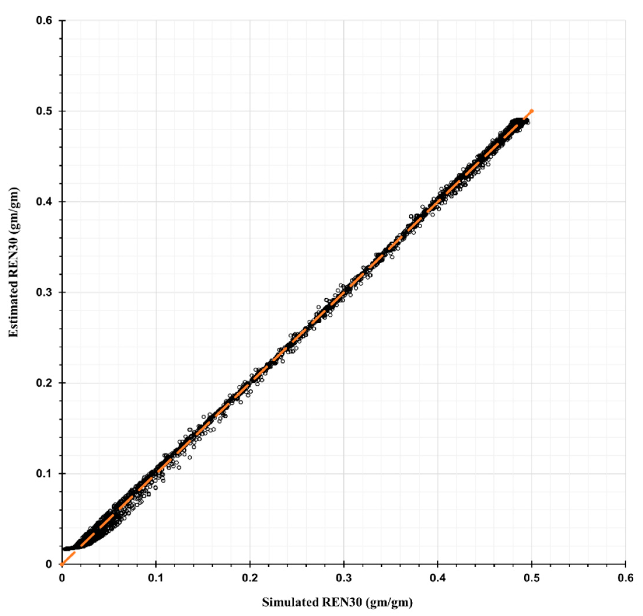
For the evaluation,

Table 3. Statistical comparisons of ANN-based estimated versus simulated REN for validation (testing) data.

Extraction Days/Parameter	15	30	45	61	76	91	Interpretation Ranges
ME (gm/gm)	−0.0000	0.0000	0.0000	0.0000	0.0002	0.0002	−∞ < ME < +∞; Perfect: 0
RMSE (gm/gm)	0.0029	0.0040	0.0081	0.0111	0.0116	0.0116	0 ≤ RMSE < +∞; Perfect: 0
PWRMSE (gm/gm)	0.0025	0.0036	0.0085	0.0120	0.0124	0.0127	0 ≤ PWRMSE < +∞; Perfect: 0
r (-)	0.9994	0.9997	0.9995	0.9994	0.9995	0.9995	−1 ≤ r ≤ 1; Perfect: 1 or −1
R2 (-)	0.9987	0.9995	0.9991	0.9988	0.9990	0.9990	0 ≤ R2 ≤ 1; Perfect: 1
ENS (-)	0.9987	0.9995	0.9991	0.9988	0.9990	0.9990	−∞ < ENS ≤ 1; Perfect: 1
|PBIAS| (%)	0.03	0.03	0.01	0.00	0.04	0.04	|PBIAS| ≤ 25% very good
SI (%)	1.47	1.11	1.64	1.92	1.80	1.74	Perfect: SI < 20%; Operational: SI < 60%

statistically shows the accuracy of the ANN-based predictors. For all extraction durations, R² values exceed 0.9987. The root mean squared error (RMSE) of the prediction that ranged from 0.0029 to 0.0127 (gm/gm) always increases with extraction duration.

To illustrate a comparison of a REN simulation with the ANN-based prediction, Figure 6 and Figure 7, Figure A1, and Figure A2 in this section and Appendix A compare simulated versus ANN-based predicted REN values for validation (testing) data and for training and validation data, respectively. In each figure, the x-axis represents the simulated and assumedly accurate REN values. The y-axis represents the ANN-based predicted REN. Perfect prediction is represented by circles lying on the diagonal line (i.e., the orange dotted line) as shown in Figure 6 and Figure 7 below.

4. Conclusions

This study provides a rapid method to predict aquifer storage and recovery (ASR) and well recovery effectiveness (REN) using artificial neural network (ANN)-based predictors. Here, REN represents the proportion of injected water molecules contained in ASR-extracted water from the same well. This is useful for balancing goals of increasing utilizable water supply while protecting aquifer environmental quality. Also, this method improves the prediction of the mass of a conservative contaminant remaining in the aquifer after a season of injection and extraction. The predicted REN values enable predicting the concentration of the extracted water that is a blend of injectate and natural background groundwater. Using the presented ANNs that apply dimensionless terms enables predicting REN for one ASR well. The well fully penetrates a homogenous, isotropic, unconfined, one-layer aquifer. The REN is predicted after every half a month of a three-month extraction period. The ANNs can be applied using a wide range of impact factor values. These ranges are aquifer hydraulic conductivity (4–20 m/d or 13.124–65.61 ft/d), porosity (0.1–0.6), specific yield (0.0375–0.57), initial (original) aquifer saturated thickness (8–46 m or 26.25–150.91 ft), initial aquifer (background) hydraulic gradient (0.00001–0.015), and steady pumping rate of injection and extraction (5.451–327.06 m³/d or 1–60 gpm). Statistics describing the accuracy of the predicted REN values after 15 to 91 days of extraction range from 0.9987 to 0.9995 for R² and 1.11 to 1.92% for scatter index (SI). The predictive REN root mean square error (RMSE) ranges from 0.0029 to 0.0116 (0.29% to 1.16%). Note, a REN could vary from near 0.00 to 1.00 (0.00 to 100%) in value.

The six ANNs share the same structure but differ in the values of the neurally associated weights. As shown statistically, the six ANN algorithms allow a user to predict REN rapidly without having to prepare for and execute numerical flow or solute transport simulations. The generated expressions make it simple and practical to evaluate ASR potential for a wide range of unconfined aquifer conditions. Assuming the presence of a pre-established groundwater right, the extraction can be continued accordingly. The simplicity of the ANNs can help water managers to rapidly perform a reconnaissance level evaluation for a candidate ASR well site. At a reconnaissance level, there might not be more than one observed hydraulic conductivity or transmissivity value in a candidate injection site.

References

- Alam, S.; Borthakur, A.; Ravi, S.; Gebremichael, M.; Mohanty, S.K. Managed aquifer recharge implementation criteria to achieve water sustainability. Sci. Total Environ. 2021, 768, 144992. [Google Scholar] [CrossRef] [PubMed]
- Daus, A.; GSI Environmental Inc. Aquifer Storage and Recovery. Improving Water Supply Security in the Caribbean Opportunities and Challenges; Discussion paper No. IDB-DP-00712; Inter-American Development Bank (IDB) Publication, Water and Sanitation Division: 2019. Available online: https://publications.iadb.org/en/aquifer-storage-and-recovery-improving-water-supply-security-caribbean-opportunities-and-challenges (accessed on 26 October 2022).
- U.S. EPA. Underground Injection Control, Aquifer Recharge, and Aquifer Storage and Recovery. 2021. Available online: https://www.epa.gov/uic/aquifer-recharge-and-aquifer-storage-and-recovery (accessed on 26 October 2022).
- Smith, W.B.; Miller, G.R.; Sheng, Z. Assessing aquifer storage and recovery feasibility in the Gulf Coastal Plains of Texas. J. Hydrol. 2017, 14, 92–108. [Google Scholar] [CrossRef]
- Bakker, M. Radial Dupuit interface flow to assess the aquifer storage and recovery potential of saltwater aquifers. Hydrogeol. J. 2010, 18, 107–115. [Google Scholar] [CrossRef]
- Pyne, R.D.G. Groundwater Recharge and Wells: A Guide to Aquifer Storage Recovery; CRC Press: Boca Raton, FL, USA, 1995. [Google Scholar]
- Brown, C.J.; Ward, J.; Mirecki, J. A Revised Brackish Water Aquifer Storage and Recovery (ASR) Site Selection Index for Water Resources Management. Water Resour. Manag. 2016, 30, 2465–2481. [Google Scholar] [CrossRef]
- Kimbler, O.K.; Kazmann, R.G.; Whitehead, W.R. Cyclic storage of freshwater in saline aquifers. In Louisiana Water Resources Research Institute Bulletin # 10; Louisiana Water Resources Research Institute: Baton Rouge, LA, USA, 1975; pp. 75–78. [Google Scholar]
- Lowry, C.S.; Anderson, M.P. An Assessment of Aquifer Storage Recovery Using Ground Water Flow Models. Ground Water 2006, 44, 661–667. [Google Scholar] [CrossRef]
- Lu, C.; Du, P.; Chen, Y.; Luo, J. Recovery efficiency of aquifer storage and recovery (ASR) with mass transfer limitation. Water Resour. Res. 2011, 47, W08529. [Google Scholar] [CrossRef]
- Pavelic, P.; Dillon, P.J.; Simmons, C.T. Multiscale Characterization of a Heterogeneous Aquifer Using an ASR Operation. Groundwater 2005, 44, 155–164. [Google Scholar] [CrossRef]
- Ward, J.D.; Simmons, C.T.; Dillon, P.J. Variable-density modelling of multiple-cycle aquifer storage and recovery (ASR): Importance of anisotropy and layered heterogeneity in brackish aquifers. J. Hydrol. 2008, 356, 93–105. [Google Scholar] [CrossRef]
- Ward, J.D.; Simmons, C.T.; Dillon, P.J.; Pavelic, P. Integrated assessment of lateral flow, density effects and dispersion in aquifer storage and recovery. J. Hydrol. 2009, 370, 83–99. [Google Scholar] [CrossRef]
- Forghani, A.; Peralta, R.C. Intelligent performance evaluation of aquifer storage and recovery systems in freshwater aquifers. J. Hydrol. 2018, 563, 599–608. [Google Scholar] [CrossRef]
- Bockelmann, A.; Zamfirescu, D.; Ptak, T.; Grathwohl, P.; Teutsch, G. Quantification of mass fluxes and natural attenuation rates at an industrial site with a limited monitoring network: A case study. J. Contam. Hydrol. 2003, 60, 97–121. [Google Scholar] [CrossRef] [PubMed]
- Ptak, T.; Piepenbrink, M.; Martac, E. Tracer tests for the investigation of heterogeneous porous media and stochastic modelling of flow and transport—A review of some recent developments. J. Hydrol. 2004, 294, 122–163. [Google Scholar] [CrossRef]
- Visser, A.; Singleton, M.J.; Esser, B.K. Xenon Tracer Test at Woodland Aquifer Storage and Recovery Well: A Report to West Yost Associates LLNL-TR-652313; Lawrence Livermore National Laboratory: Livermore, CA, USA, 2014.
- Fitts, C.R. Uncertainty in deterministic groundwater transport models due to the assumption of macrodispersive mixing: Evidence from the Cape Cod (Massachusetts, U.S.A.) and Borden (Ontario, Canada) tracer tests. Contam. Hydrol. 1996, 23, 69–84. [Google Scholar] [CrossRef]
- Khaki, M.; Yusoff, I.; Islami, N. Application of the artificial neural network and neuro-fuzzy system for assessment of groundwater quality. Clean Soil Air Water 2015, 43, 551–560. [Google Scholar] [CrossRef]
- Nordin, N.F.C.; Mohd, N.S.; Koting, S.; Ismail, Z.; Sherif, M.; EL-Shafie, A. Groundwater quality forecasting modelling using artificial intelligence: A review. Groundw. Sustain. Dev. 2021, 14, 100643. [Google Scholar] [CrossRef]
- Sakizadeh, M. Artificial intelligence for the prediction of water quality index in groundwater systems. Model. Earth Syst. Environ. 2016, 2, 8. [Google Scholar] [CrossRef]
- Haykin, S. Neural Networks: A Comprehensive Foundation, 2nd ed.; Prentice Hall: Upper Saddle River, NJ, USA, 1994. [Google Scholar]
- Sahoo, G.B.; Ray, C.; Mehnert, E.; Keefer, D.A. Application of artificial neural networks to assess pesticide contamination in shallow groundwater. Sci. Total Environ. 2006, 367, 234–251. [Google Scholar] [CrossRef] [PubMed]
- Sahoo, G.B.; Ray, C.; Wade, H.F. Pesticide prediction in ground water in North Carolina domestic wells using artificial neural networks. Ecol. Model. 2005, 183, 29–46. [Google Scholar] [CrossRef]
- De Vos, N.J.; Rientjes, T.H.M. Constraints of artificial neural networks for rainfall-runoff modelling: Trade-offs in hydrological state representation and model evaluation. Hydrol. Earth Syst. Sci. Discuss. 2005, 2, 365–415. [Google Scholar] [CrossRef] [Green Version]
- Coulibaly, P.; Anctil, F.; Aravena, R.; Bobee, B. Artificial neural network modeling of water table depth fluctuations. Water Resour. Res. 2001, 37, 885–896. [Google Scholar] [CrossRef] [Green Version]
- Daliakopoulos, I.N.; Coulibaly, P.; Tsanis, I.K. Groundwater level forecasting using artificial neural networks. J. Hydrol. 2005, 309, 229–240. [Google Scholar] [CrossRef]
- Malik, A.; Bhagwat, A. Modelling groundwater level fluctuations in urban areas using artificial neural network. Groundw. Sustain. Dev. 2021, 12, 100484. [Google Scholar] [CrossRef]
- Kuo, Y.; Liu, C.; Lin, K. Evaluation of the ability of an artificial neural network model to assess the variation of groundwater quality in an area of blackfoot disease in Taiwan. Water Res. 2004, 38, 148–158. [Google Scholar] [CrossRef] [PubMed]
- Liu, H.; Li, J.; Cao, H.; Xie, X.; Wang, Y. Prediction modeling of geogenic iodine contaminated groundwater throughout China. J. Environ. Manag. 2022, 303, 114249. [Google Scholar] [CrossRef]
- Banerjee, P.; Singh, V.S.; Chatttopadhyay, K.; Chandra, P.C.; Singh, B. Artificial neural network model as a potential alternative for groundwater salinity forecasting. J. Hydrol. 2011, 398, 212–220. [Google Scholar] [CrossRef]
- Govindaraju, R.S. Artificial Neural Networks in Hydrology. II: Hydrologic Applications, By the ASCE Task Committee on Application of Artificial Neural Networks in Hydrology. J. Hydrol. Eng. 2000, 5, 124–137. [Google Scholar] [CrossRef]
- Maren, A.; Harston, C.; Pap, R. Handbook of Neural Computing Applications; Academic Press: San Diego, CA, USA, 1990. [Google Scholar]
- Hagan, M.T.; Demuth, H.B.; Beale, M.H. Neural Network Design; PWS Publishing Co.: Boston, MA, USA, 1996. [Google Scholar]
- Mezard, M.; Nadal, J.P. Learning in feedforward layered networks: The tiling algorithm. J. Phys. A Math. Gen. 1989, 22, 2191–2203. [Google Scholar] [CrossRef] [Green Version]
- Gunther, F.; Fritsch, S. Neuralnet: Training of Neural Networks. R J. 2010, 2, 30–38. [Google Scholar] [CrossRef] [Green Version]
- Fetter, C.W. Contaminant Hydrogeology, 2nd ed.; Prentice-Hall Inc.: Upper Saddle River, NJ, USA, 1999; pp. 73–74. [Google Scholar]
- Bedient, P.B.; Rifai, H.S.; Newell, C.J. Ground Water Contamination, Transport and Remediation, 2nd ed.; Prentice-Hall Inc.: Upper Saddle River, NJ, USA, 1999; pp. 179–180. [Google Scholar]
- Lambert, P.M. Numerical Simulation of Ground-Water Flow in Basin-Fill Material in Salt Lake Valley, Utah. United States Geological Survey, Technical Publication No. 110-B 1995. Available online: https://pubs.er.usgs.gov/publication/70179464 (accessed on 24 August 2007).
- Gelhar, L.W.; Welty, C.; Rehfeldt, K.R. A Critical Review of Data on Field-Scale Dispersion in Aquifers. Water Resour. Res. 1992, 28, 1955–1974. [Google Scholar] [CrossRef]
- Heath, R.C. Basic Ground-Water Hydrology. United States Geological Survey. Water-Supply Pap. 1983, 2200, 84. [Google Scholar]
- iUTAH, Innovate Urban Transitions and Arid Region Hydro-Sustainability. 2012. Available online: https://iutahepscor.org/ (accessed on 13 July 2012).
- McDonald, M.G.; Harbaugh, A.W. A Modular Three-Dimensional Finite-Difference Ground-Water Flow Model; United States Geological Survey Report, Techniques of Water-Resources Investigations 06-A1; US Geological Survey: Liston, VA, USA, 1988. [CrossRef]
- Zheng, C.; Wang, P.P. MT3DMS: A Modular Three-Dimensional Multispecies Transport Model for Simulation of Advection, Dispersion, and Chemical Reactions of Contaminants in Groundwater Systems: Documentation and User’s Guide. In U.S. Army Engineer Research and Development Center Cataloging-in-Publication Data, Final Report, Contract Report SERDP-99-1; US Army Engineer Research and Development Center: Vicksburg, MS, USA, 1999. [Google Scholar]
- U.S. EPA. Online Tools for Site Assessment Calculation. U.S. Environmental Protection Agency. 2019. Available online: https://www3.epa.gov/ceampubl/learn2model/part-two/onsite/longdisp.html (accessed on 31 August 2021).
- Wilson, J.L.; Conrad, S.H.; Mason, W.R.; Peplinski, W.; Hagan, E. Laboratory Investigation of Residual Liquid Organics; 600/6-90/004; United States Environmental Protection Agency: Ada, OK, USA, 1990.
- Xu, M.; Eckstein, Y. Use of Weighted Least-Squares Method in Evaluation of the Relationship between Dispersivity and Field Scale. Ground Water 1995, 33, 905–908. [Google Scholar] [CrossRef]
- Daus, A.D.; Frind, E.O.; Sudicky, E.A. Comparative error analysis in finite element formulations of the advection-dispersion equation. Adv. Water Resour. 1985, 8, 86–95. [Google Scholar] [CrossRef]
- Macpherson, G.L.; Townsend, M.A. Perspectives on Sustainable Development of Water Resources in Kansas, Chapter 5: Water Chemistry and Sustainable Yield. Kansas Geological Survey Bulletin 239. 1998. Available online: https://www.kgs.ku.edu/Publications/Bulletins/239/Macpherson/index.html (accessed on 27 May 2013).
- Gropp, W.; Lusk, E.; Skjellum, A. Using MPI: Portable Parallel Programming with the Message-Passing Interface, 3rd ed.; MIT Press: Cambridge, MA, USA, 2014. [Google Scholar]
- Ketabchi, H.; Ataie-Ashtiani, B. Assessment of a parallel evolutionary optimization approach for efficient management of coastal aquifers. Environ. Model. Softw. 2015, 74, 21–38. [Google Scholar] [CrossRef]
- Neal, J.C.; Fewtrell, T.J.; Bates, P.D.; Wright, N.G. A comparison of three parallelization methods for 2D flood inundation models. Environ. Model. Softw. 2010, 25, 398–411. [Google Scholar] [CrossRef]
- Sloan, J.D. High Performance Linux Clusters: With OSCAR, Rocks, OpenMosix, and MPI: A Comprehensive Getting-Started Guide; O’Reilly Media, Inc.: Newton, MA, USA, 2009. [Google Scholar]
- Snir, M.; Otto, S.; Huss-Lederman, S.; Walker, D.; Dongarra, J. MPI: The Complete Reference; The MIT Press: Cambridge, MA, USA, 1996. [Google Scholar]
- Bear, J. Some Experiments in Dispersion. J. Geophys. Res. 1961, 66, 2455–2467. [Google Scholar] [CrossRef]
- Freeze, R.A.; Cherry, J.A. Groundwater; Prentice Hall Inc.: Upper Saddle River, NJ, USA, 1979; p. 604. [Google Scholar]
- U.S. EPA. A Systematic Approach for Evaluation of Capture Zones at Pump and Treat Systems; EPA/600/R-08/003; U.S. Environmental Protection Agency: Washington, DC, USA, 2008.
- Dreyfus, G. Neural Networks: Methodology and Applications; Springer: Berlin/Heidelberg, Germany, 2005; pp. 135–137. [Google Scholar]
- Hornik, K.; Stinchcombe, M.; White, H. Multilayer feedforward networks are universal approximators. Neural Netw. 1989, 2, 359–366. [Google Scholar] [CrossRef]
- Priddy, K.L.; Keller, P.E. Artificial Neural Networks: An Introduction; SPIE PRESS, The International Society for Optical Engineering: Bellingham, WA, USA, 2005. [Google Scholar]
- Schmidhuber, J. Deep learning in neural networks: An overview. Neural Netw. 2015, 61, 85–117. [Google Scholar] [CrossRef] [Green Version]
- Cooper, H.H., Jr.; Jacob, C.E. A Generalized Graphical Method for Evaluating Formation Constants and Summarizing Well-Field History. Trans. Am. Geophys. Union 1946, 27, 526–534. [Google Scholar] [CrossRef]
- Jacob, C.E. Notes on determining permeability by pumping tests under water table conditions. United States Geological. Survey Open-file Report, Effective radius of drawdown test to determine artesian well. Am. Soc. Civil Eng. Proc. 1944, 72, 629–646. [Google Scholar]
- Fitts, C.R. Groundwater Science; Academic Press; Elsevier Science: Cambridge, MA, USA, 2002; pp. 221–235. [Google Scholar]
- Huisman, L. Groundwater Recovery; Winchester Press and the Macmillan Press: New York, NY, USA, 1972; pp. 206–211. [Google Scholar]
- Neuman, S.P. Analysis of Pumping Test Data from Anisotropic Unconfined Aquifers Considering Delayed Gravity Response. Water Resour. Res. 1975, 11, 329–342. [Google Scholar] [CrossRef]
- Schwartz, F.W.; Zhang, H. Fundamentals of Groundwater; John Wiley and Sons Inc.: Hoboken, NJ, USA, 2003; pp. 258–270. [Google Scholar]
- Javan, K.; Fallah Haghgoo Lialestani, M.R.; Nejadhossein, M. A comparison of ANN and HSPF models for runoff simulation in Gharehsoo River watershed, Iran. Model. Earth Syst. Environ. 2015, 1, 41. [Google Scholar] [CrossRef] [Green Version]
- Mentaschi, L.; Besio, G.; Cassola, F.; Mazzino, A. Problems in RMSE-based wave model validations. Ocean Model. 2013, 72, 53–58. [Google Scholar] [CrossRef]
- Jimeno-Sáez, P.; Senent-Aparicio, J.; Pérez-Sánchez, J.; Pulido-Velazquez, D. A Comparison of SWAT and ANN Models for Daily Runoff Simulation in Different Climatic Zones of Peninsular Spain. Water 2018, 10, 192. [Google Scholar] [CrossRef] [Green Version]
- Moriasi, D.N.; Arnold, J.G.; Van Liew, M.W.; Bingner, R.L.; Harmel, R.D.; Veith, T.L. Model Evaluation Guidelines for Systematic Quantification of Accuracy in Watershed Simulations. Soil Water Div. Am. Soc. Agric. Biol. Eng. 2007, 50, 885–900. [Google Scholar] [CrossRef]
- Nash, J.E.; Sutcliffe, J.V. River flow forecasting through conceptual models: Part 1, A discussion of principles. J. Hydrol. 1970, 10, 282–290. [Google Scholar] [CrossRef]
- Janssen, P.A.E.M.; Komen, G.J. An Operational Coupled Hybrid Wave Prediction Model. Geophys. Res. 1984, 89, 3635–3654. [Google Scholar] [CrossRef]
Figure 1.
Schematic diagram of ANN structure including the input layer, one hidden layer, and the output layer.
Figure 2.
MODFLOW2005-MT3DMS model study area for ASR well, top view (not to scale).
Figure 3.
MODFLOW2005-MT3DMS model study area for ASR well, side view (not to scale).
Figure 4.
Schematic diagram of ANN structure including three-term inputs, one neuron, REN output for a specific time, and associated weighting coefficients.
Figure 5.
Scheme of 10-fold cross validation method for the data set of ANN.
Figure 6.
Comparison of ANN-based predicted versus simulated REN30 for validation (testing) data.
Figure 7.
Comparison of ANN-based predicted versus simulated REN91 for validation (testing) data.