Meteorological Knowledge Useful for the Improvement of Snow Rain Separation in Surface Based Models

Abstract

An accurate precipitation phase determination—i.e., solid versus liquid—is of paramount importance in a number of hydrological, ecological, safety and climatic applications. Precipitation phase can be determined by hydrological, meteorological or combined approaches. Meteorological approaches require atmospheric data that is not often utilized in the primarily surface based hydrological or ecological models. Many surface based models assign precipitation phase from surface temperature dependent snow fractions, which assume that atmospheric conditions acting on hydrometeors falling through the lower atmosphere are invariant. This ignores differences in phase change probability caused by air mass boundaries which can introduce a warm air layer over cold air leading to more atmospheric melt energy than expected for a given surface temperature, differences in snow grain-size or precipitation rate which increases the magnitude of latent heat exchange between the hydrometers and atmosphere required to melt the snow resulting in snow at warmer temperatures, or earth surface properties near a surface observation point heating or cooling a shallow layer of air allowing rain at cooler temperatures or snow at warmer temperatures. These and other conditions can be observed or inferred from surface observations, and should therefore be used to improve precipitation phase determination in surface models.

1. Introduction

The hydrological, ecological, and atmospheric responses to rain are extremely different from snow responses [1] and correct precipitation phase is, therefore, very important for applications across many scientific fields. Truthful identification of the precipitation phase (rain/snow) is of course crucial for the functioning of meteorological models that forecast the precipitation phase itself [2] but also for accurate correction of gauge measured winter precipitation [3] and for land surface models (LSM) predicting snow accumulation and melt [4], glacier and polar ice water balance models [5], models for lake and sea ice growth [6], and climate change models [7]. It is also important for models predicting avalanche hazards [8], sublimation of snow in forests [9], urban snowmelt quality [10], winter road safety [11], infiltration into frozen soils [12], survival of mammals and plants under snow cover [13], flooding from rain on snow events [14] etc. Precipitation phase determination is a modeling challenge for both hydrology and meteorology; therefore, a cross discipline approach combining methods and knowledge from both sciences could lead to new insight for both.

The International Association of Hydrological Sciences Decade on Prediction in Ungauged Basins (PUB) had the goal to improve basin hydrology through understanding processes rather than simply calibrating modeling schemes [15,16]. In ungauged basins, knowledge of processes would create more robust hydrological solutions compared to the traditional approach to calibrate parameters in one basin, and apply them in others without adjustments for landscape heterogeneity [15]. An example of a calibrated parameter used in many hydrological models is the precipitation phase determination scheme (PPDSs) usually based on surface temperature (the 2 m temperature reported from surface meteorological stations) relationships, ignoring important landscape and atmospheric interactions [17]. For example, compared to dry landscapes, open water and unfrozen wetlands add heat and moisture to sub or near freezing air in the lowest part of the atmosphere introducing variability into average atmospheric conditions across landscapes. For this reason, ice-free oceans were found to have a warmer PPDS threshold temperature than continental landscapes [18,19]. Therefore, it should be accepted that different PPDS schemes will be needed to account for lower atmospheric differences caused by variations in landscape. For example, dew point temperature based PPDS yielded less error than air temperature based PPDS in a saturated mountain environment [20], but an air temperature PPDS performed better in lower drier landscapes [21].

Within hydrological models, the PPDS are important [22], and many different schemes have been used. The most common approaches use surface air temperature (T_A) e.g., [23] to determine the precipitation phase. Often T_A and precipitation mass are the only measured variables with either lengthy enough historical records, or available at enough measuring stations for many studies requiring a PPDS [24]. Unfortunately, T_A methods are not physically based as they do not attempt to incorporate physical processes present in the real world e.g., the effects of humidity on latent heat transfer [25] and other hydrometeor processes above the soil surface [26]. There are a few hydrological models that attempt to account for moisture in the surface-based PPDS by using surface dew point temperature (T_D) [20], surface wet bulb temperature (T_W) [27], and surface relative humidity (RH) [1].

All surface-based PPDS approaches assume a constant decrease in air temperature with height (e.g., the Climate High Resolution Model (CHRM)—7.5 °C/km) [16] and do not account for interactions either between warm and cold air masses found in the most basic mid-latitude cyclone theories, or between hydrometeors and the air as precipitation falls through the lower atmosphere [28]. Therefore, without atmospheric measurements, the most physically based surface PPDS methods can not accurately reproduce physical processes occurring between hydrometeors and the atmosphere they fall through. The phase of precipitation at the ground can be univocally determined only by knowing the initial hydrometeor phase [29], hydrometeor shape and size [26], and the properties of the atmosphere through which the hydrometeor falls. These properties include above ground air temperatures (T_AG), height of the 0 °C isotherm (Z0 °C) [17], vertical thickness of freezing and melting layers [26], atmospheric humidity [1], atmospheric stability [30], and interactions between hydrometeors [2,25,29,31].

The equations used for describing the microphysical processes evaporation, sublimation, freezing, and melting [26,29] acting on the falling hydrometeors are calculation intensive and require detailed atmospheric information often not included in current hydrological models [29].

However, some hydrological modelers have begun to integrate meteorological measurements, or add steps that indirectly account for atmospheric changes into their PPDS. These methods use T_A, T_AG, weather radars, or satellite images. Fassnacht et al. [32] and Gjertsen and Ødegaard [33] e.g., improved precipitation mass by integrating radar precipitation estimates into their hydrological models. However, they chose to use surface T_A methods rather than differences in the properties of the radar return pulse that could distinguish precipitation phase.

This paper reviews and analyses studies dealing with precipitation phase processes and methods to determine the phase with an aim to suggest approaches that will improve the separation of rain and snow in cold region hydrological models. It starts with a basic overview of fundamental meteorological knowledge to build a baseline understanding of the physical changes between hydrometeors and air in the lower atmosphere. This first section builds to explain terrain/landscape, precipitation rate, and frontal boundary effects on the atmospheric temperature/moisture with height which has an impact on energy needed to drive phase changes in precipitation. This is followed by a short review of PPDS in atmospheric models and a longer review of current PPDS methods in surface models. The advantages and disadvantages of these PPDS methods are discussed along with a proposed formula to simplify surface air temperature–relative humidity PPDS schemes.

2. Atmospheric Interactions during Phase Change

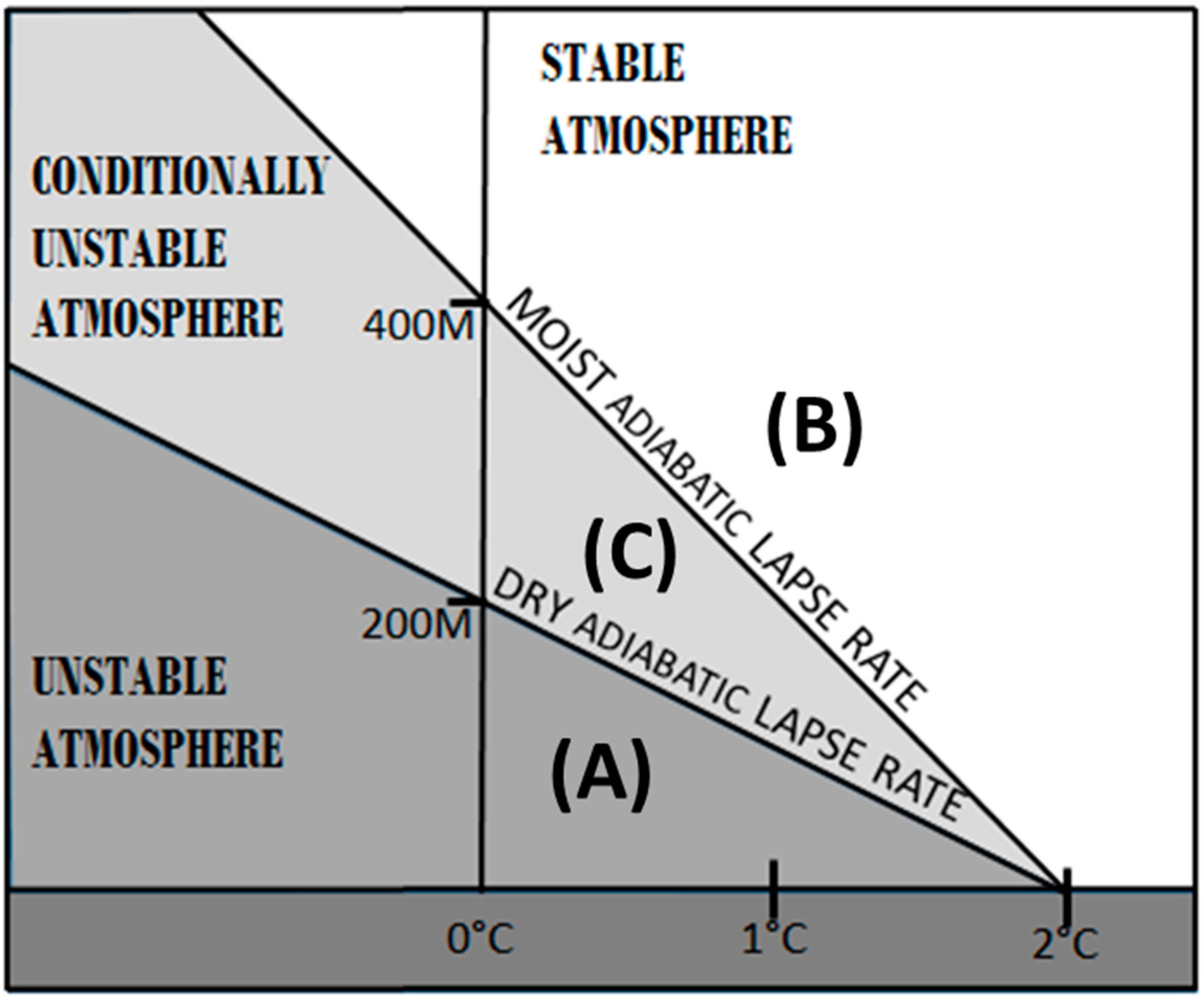
In general, clouds and precipitation form when an air parcel rises and cools to saturation at the condensation level (the base of clouds). If snow falls through a warm atmospheric layer (>0.0 °C) melting will begin [25,32]. Depending on air temperature, humidity and the thickness of a warm layer, latent and sensible heat exchanges between the snow and atmosphere could cause phase change from dry snow, to wet snow, to slush, to rain [26,32,34].

Hydrological models based on surface weather observations do not have enough information to construct a vertical temperature/moisture profile that accurately reflects atmospheric conditions above the surface. A precipitation phase reported from a point location could be the result of many different atmospheric processes e.g., Stewart [25] explained that melting snow at the surface can be a result of (1) the melting process; (2) heat gained from collision with rain drops; (3) refreezing after partial melt; or (4) collisions with supercooled water. The assumption of any of these processes extrapolated over a model surface could lead to large errors. Therefore, the use of a vertical temperature/moisture profile of the environment is preferred in meteorology because it can first determine which hydrometeors are most likely to form in clouds, and then calculate any precipitation phase changes that might occur between and below the cloud level at which the hydrometeor formed.

2.1. Lapse Rates

Sampling instruments carried by weather balloons known as radiosondes provide vertical profiles of above ground air pressure, air temperature, dew point, wind speed/direction, and GPS location. Spatial resolution of the observations depends on the number of balloons launched in a given area. Over 800 stations worldwide submit radiosonde data for model intake. The time resolution is twice a day [35] at most locations. The vertical temperature and moisture profile gives useful information; e.g., freezing level height, actual lapse rate compared to the dry and moist adiabatic lapse rates [17], (Figure 1), and the depth of melting and freezing layers. Another reason to use radiosonde data for this application is that T_A varies more than T_AG since the Earth’s surface absorbs ultraviolet solar radiation and emits infrared radiation at different rates through the day. However, representative vertical temperature profiles may not be available at a necessary time, or for some areas the closest observation is hundreds of kilometers away and may not be representative for terrain or landscape induced variations in the lower atmosphere.

2.2. Deviations from Average Lapse Rates

The vertical temperature lapse rate under dry atmospheric conditions can be assumed to decrease steadily with height (Figure 2A). A similar assumption is implied through the use of set T_A thresholds in hydrological models. These assumptions are incorrect when one or more of the following occurs in the near surface atmosphere; (a) the lapse rate is more unstable than average, decreasing the expected depth of a near surface warm layer (Figure 1); (b) there is an air mass boundary (Figure 2B,C); (c) falling snow is melting or refreezing (Figure 3); and (d) evaporation, sublimation, and/or condensation is occurring.

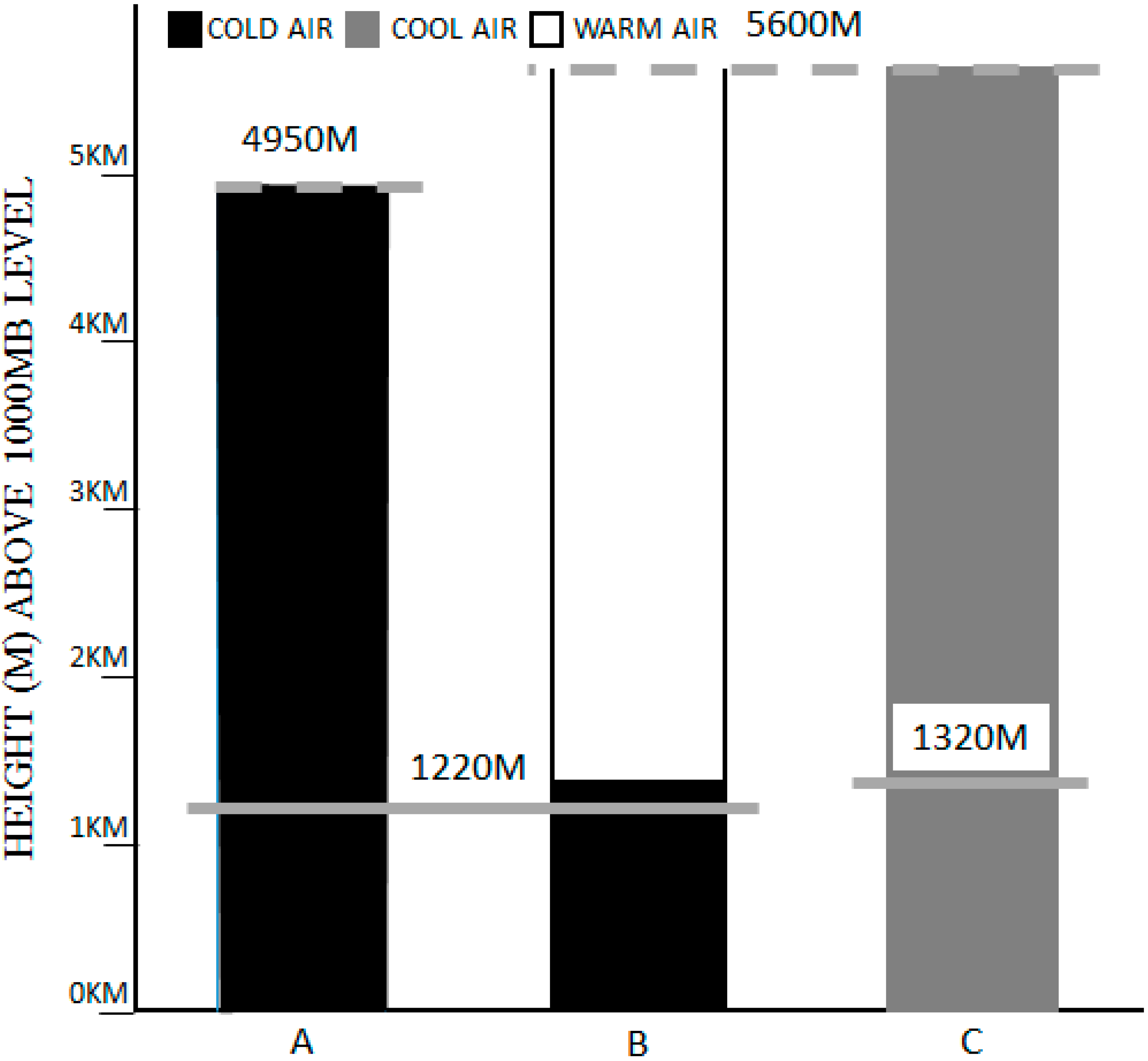
2.2.1. Air Mass Boundaries

Air mass boundaries introduce deviation from expected lapse rates due to a sharp increase or decrease in T_AG (Figure 2B,C). For a given T_A, this changes the probability of snow melting before reaching the ground.

Figure 1. Dry (9.8 °C/km) and moist (5.9 °C/km) adiabatic lapse rates, give the expected cooling rates for rising air parcels without moisture or temperature advection. The dry and moist adiabatic lapse rates characterize the actual lapse rate as: (A) unstable when the actual T_AG decrease is ≥ the dry adiabatic lapse rate (9.8 °C/km). Here, an air parcel that is warmed or lifted will be lighter than the surrounding air and rise whether it is moist or dry. (B) stable when the actual T_AG decrease is ≤ the moist adiabatic lapse rate (5.9 °C/km). Here, an air parcel forced to higher altitudes (by terrain, or frontal lift) will be more dense than the surrounding atmosphere and will have a tendency to sink, even if condensation occurs; (C) conditionally unstable when the actual T_AG decrease is between 5.9 and 9.8 °C/km. Here, an air parcel must be forced to higher altitudes (over terrain or a frontal slope) to reach its condensation temperature. From that altitude, the moist adiabatic lapse rate decreases slower than the actual lapse rate. Therefore, an air parcel can become lighter than the surrounding air and rise freely.

Figure 1. Dry (9.8 °C/km) and moist (5.9 °C/km) adiabatic lapse rates, give the expected cooling rates for rising air parcels without moisture or temperature advection. The dry and moist adiabatic lapse rates characterize the actual lapse rate as: (A) unstable when the actual T_AG decrease is ≥ the dry adiabatic lapse rate (9.8 °C/km). Here, an air parcel that is warmed or lifted will be lighter than the surrounding air and rise whether it is moist or dry. (B) stable when the actual T_AG decrease is ≤ the moist adiabatic lapse rate (5.9 °C/km). Here, an air parcel forced to higher altitudes (by terrain, or frontal lift) will be more dense than the surrounding atmosphere and will have a tendency to sink, even if condensation occurs; (C) conditionally unstable when the actual T_AG decrease is between 5.9 and 9.8 °C/km. Here, an air parcel must be forced to higher altitudes (over terrain or a frontal slope) to reach its condensation temperature. From that altitude, the moist adiabatic lapse rate decreases slower than the actual lapse rate. Therefore, an air parcel can become lighter than the surrounding air and rise freely.

2.2.2. Isothermal Layers

Melting and refreezing of falling snow causes a near-freezing (+0 °C) isothermal layer (D_melt) due to sensible and latent heat exchanges (Figure 3) [36]. This isothermal layer provides limited energy for phase changes, reducing the total amount of melting or refreezing caused by atmosphere-hydrometeor energy exchanges.

2.2.3. Precipitation Intensity and Duration

The depth of D_melt increases with precipitation intensity and duration (Figure 3) [17,33,36]. Minder et al. [17] found that D_melt for very light precipitation was about 60 m and could exceed 300 m for high precipitation rates.

Figure 2. Examples of vertical air temperature profiles: (A) a single air mass with a constant lapse rate; (B) an air mass boundary separating a warm over cold air mass; and (C) an air mass boundary separating a cold over warm air mass.

Figure 2. Examples of vertical air temperature profiles: (A) a single air mass with a constant lapse rate; (B) an air mass boundary separating a warm over cold air mass; and (C) an air mass boundary separating a cold over warm air mass.

Gjertsen and Ødegaard’s [33] found that the above ground T_W lapse rate decreased with increasing precipitation rates from 0.6 to 0.1 °C/100 m. The maximum D_melt was 598 m, and the minimum was 244 m. However, Minder et al. [17] claims that D_melt is not an important factor since strong frontal winds usually restrict the average residency period of air in a melting layer to 10 min.

Snow fractions for a given T_A can be expected to increase with precipitation intensity and storm duration (Figure 3). Figure 3 illustrates differences between typical low intensity and short duration storms (Figure 3A) and high intensity or long duration storms (Figure 3B).

2.2.4. Evaporation, Sublimation and Condensation

Melting causes a D_melt to form in the vertical profile that is usually a few hundred meters deep [37,38]. The thickness of D_melt is dependent on snowflake diameter, relative humidity (RH), precipitation rate, and the atmospheric lapse rate [17]. Mitra et al. [39] demonstrated that a 10 mm diameter snowflake would have a D_melt 100 m thicker than a 5 mm snowflake during otherwise identical conditions. The sensible flux is dependent on the temperature difference between the hydrometeor and the ambient air while the latent heat flux is reliant upon the difference in vapor density (i.e., on RH) between the hydrometeor and the ambient air [20,29]. Sublimation (2594 J/g) and evaporation (2260 J/g) consume heat energy from the atmosphere reducing available melt energy (334 J/g) while condensation (2260 J/g), ice condensation (2594 J/g), and freezing (334 J/g) release heat energy back into the atmosphere. Melting and refreezing may be combined with evaporation/sublimation, so that hydrometeor latent and sensible heat exchange is balanced by heat flux from the atmosphere. For moist air, i.e., air with high relative humidity, little evaporation/sublimation can be expected due to high vapor density surrounding the hydrometeor while more can be expected for dry air due to low vapor density around the hydrometeor [29].

Figure 3. Overviews of flat areas are shown to the right in the two Figure 3A,B where initial storm conditions are the same but precipitation rate and duration differ. From bottom to top in the overview, surface temperatures increase to correspond with a precipitation phase change from snow to mixed precipitation to rain. The vertical profiles to the left in the subfigures illustrate the situation in location 2; (A) illustrates the situation for a low intensity or the beginning of a precipitation event, with a thin isothermal layer in the vertical temperature profile; (B) illustrates the situation for a prolonged or high precipitation intensity event. It has increased depth of the isothermal layer but minor change in surface temperature, a more unstable near surface lapse rate, decreasing melt and increasing surface snow areas.

Figure 3. Overviews of flat areas are shown to the right in the two Figure 3A,B where initial storm conditions are the same but precipitation rate and duration differ. From bottom to top in the overview, surface temperatures increase to correspond with a precipitation phase change from snow to mixed precipitation to rain. The vertical profiles to the left in the subfigures illustrate the situation in location 2; (A) illustrates the situation for a low intensity or the beginning of a precipitation event, with a thin isothermal layer in the vertical temperature profile; (B) illustrates the situation for a prolonged or high precipitation intensity event. It has increased depth of the isothermal layer but minor change in surface temperature, a more unstable near surface lapse rate, decreasing melt and increasing surface snow areas.

2.2.5. Hydrometeor Interactions

If droplets freeze or ice crystals melt on a hydrometeor, they would release or absorb 334 J/g of latent heat [25]. The melting rate of snowflakes thus increases when they collide with cloud or rain droplets [26]. This is because a hydrometeor composed of both liquid and solid fractions has a fixed temperature of 0 °C [25]. Snow colliding with rain or cloud droplets will undergo melting to chill the droplets to 0 °C [25].

The atmospheric physics of hydrometeor formation and interactions including phase change are very complicated. An understanding of the basic five equation microphysical schemes used by Stewart [25] is suggested. His equations account for: (1) Heat exchange resulting from gas, liquid, or solid phase change; (2) Change in particle mass by condensation; (3) The resulting latent heat flux from condensation; (4) Heat exchange from collision coalescence or through accretion of liquid and ice crystals; and (5) Latent heat of fusion with particles melting or freezing due to contact with each other. Detailed examples of more complicated microphysical schemes are found in e.g., Thériault and Stewart [26] or Lundquist [28].

2.2.6. Terrain Influence

Topography plays an important role in the surface location of rain/snow phase transitions. It is common for phase transition to be associated with a shallow cold layer beneath a warm layer on the lee side of mountains. This is known as cold air damming. This phenomenon can lower Z0 °C [17,25], and may add an extra freezing level in the vertical temperature profile (Figure 4). A phase transition region can sometimes be linked to coastlines due to warm sea surface temperatures. The warm water transfers heat to the near surface atmosphere increasing the available melt energy over the open water, also extending into the near coastal region. Strong winds can push this warm air further inland or offshore, therefore, also moving the location of a phase transition region [25]. In most cases, a phase transition region will progress towards adjacent rain areas (Figure 3) [25].

Figure 4. Phase changes of snow in a melting layer, followed by phase changes in a refreezing layer modified from [26].

Figure 4. Phase changes of snow in a melting layer, followed by phase changes in a refreezing layer modified from [26].

Air forced to rise over terrain obstacles may also yield orographically enhanced precipitation. Increased precipitation rates cause a thicker D_melt, lower Z0 °C and snow elevation (Z_S) than upwind [17]. This lowering of Z0 °C and Z_S will introduce phase errors in a model that simply projects temperature heights from a sounding (or snow elevations from radar returns) without adjusting for variations in terrain. The magnitude of change in Z0 °C and Z_S depends on the geometry of the terrain and the properties of the melting layer (including both RH and wind speed) [17].

3. Atmospheric Precipitation Phase Determination

Most meteorological PPDS approaches are based on measured atmospheric conditions. There are many approaches that range from complex bulk microphysical schemes to simplified empirical approaches using thickness values or freezing levels to determine phase.

Snow, wet snow, and/or rain might form when T_AG decreases with height, while, a T_AG profile consisting of a warm layer (>0 °C) aloft and a cold layer below (<0 °C) usually is needed to form ice pellets, supercooled rain, and freezing rain (Figure 4) [26].

3.1. Bulk Microphysical Schemes

Meteorological models commonly use bulk microphysical schemes to determine the hydrometeor phase as precipitation falls to the surface. These schemes assume a size distribution for hydrometeors [26]. A hydrometeor’s size determines the amount of energy needed for phase change. Small hydrometeors changing phase faster than large hydrometeors is often the cause of mixed phase precipitation [26,29].

There are both sophisticated and simplified bulk microphysical schemes (Table 1). The sophisticated Purdue-Lin scheme incorporates six hydrometeor classes (water vapor, cloud water, cloud ice, rain, snow, and graupel) and mixed-phase processes [40]. This scheme applies complex equations to account for evaporation, sublimation, deposition, condensation, aggregation, accretion, Bergeron processes, freezing, and melting. Other bulk microphysical schemes are simpler, e.g., the WSM3 (WFR [Weather Research and Forecasting] Single Moment-3) with three precipitation phases [41] that does not allow mixed phase processes, assuming an instantaneous phase changes to occur at freezing levels.

Table 1. WRF Model Version 3 Microphysical Schemes from most to least complex table modified from [42].

Microphysical Scheme	Precipitation Types	Allows Mixed Phase Processes
Morrison 2-Moment	10	Yes
Thompson	7	Yes
Goddard	6	Yes
Purdue Lin	6	Yes
WSM6	6	Yes
WSM5	5	No
WSM3	3	No
Kessler	3	No
Eta GCP	2	Yes

Table 1. WRF Model Version 3 Microphysical Schemes from most to least complex table modified from [42].

Microphysical Scheme	Precipitation Types	Allows Mixed Phase Processes
Morrison 2-Moment	10	Yes
Thompson	7	Yes
Goddard	6	Yes
Purdue Lin	6	Yes
WSM6	6	Yes
WSM5	5	No
WSM3	3	No
Kessler	3	No
Eta GCP	2	Yes

Of note, most microphysical schemes do not account for drizzle formed through the warm rain process in low clouds, usually under inversions. These clouds contain little ice condensation nuclei causing supercooled drizzle without the melting and refreezing layers in Figure 4 [1,33].

3.2. Empirical Phase Determination Schemes

3.2.1. Thickness Values

A thickness value is the difference in height (D_Z) between two standard pressure levels (e.g., between 500 and 1000 mb) identified by Radiosonde data. D_Z is proportional to the changes in pressure (D_P) and density. Given a constant D_P, warm air is less dense resulting in a larger D_Z, while, cold air has the opposite properties (Figure 5). Critical thickness values e.g., 1300 m for 1000–850 mb, 2840 m for 1000–700 mb and 5400 m for 1000–500 mb [43] can be used as rain/snow thresholds. Snow is expected when a D_Z is lower than the critical D_Z value, and rain if a D_Z is higher. Meteorology traditionally used critical D_Z values [25,43] when less computational PPDS methods were necessary (Figure 5). The advantage of this method is its simplicity. It is less sensitive to diurnal change than T_A but still has many of the same disadvantages. Specifically this method assumes a constant or average change in temperature with height (Figure 2A, Figure 5A,C) but cannot identify cold, warm, (Figure 2B,C and Figure 5B) or isothermal layers (Figure 3B) in the vertical temperature profile affecting precipitation phase [25].

Figure 5. Example of thickness values (D_Z) for 1000 to 850 mb (solid line), and for 1000 to 500 mb (hatched line) for air columns with (A) a cold air mass; (B) an air mass boundary and (C) a warm air mass.

Figure 5. Example of thickness values (D_Z) for 1000 to 850 mb (solid line), and for 1000 to 500 mb (hatched line) for air columns with (A) a cold air mass; (B) an air mass boundary and (C) a warm air mass.

3.2.2. Freezing Levels

The height of Z0 °C is available from radiosonde data and is also used to determine the probability of snow falling through a near surface warm layer (Table 2). Similar approaches exist for above ground T_W and T_D.

Table 2. Probability of snow based on the height of the freezing layer (T_AG = 0 °C).

Freezing Layer Height (m)*	0	95	200	280	365
Snow Probability (%)	100	90	70	50	0

* Converted from feet [44] to the nearest 5 m.

Table 2. Probability of snow based on the height of the freezing layer (T_AG = 0 °C).

Freezing Layer Height (m)*	0	95	200	280	365
Snow Probability (%)	100	90	70	50	0

* Converted from feet [44] to the nearest 5 m.

On average, a warm layer must be at least 1200 ft (365 m) thick to completely melt all snow [43]. This approach does not account for the following factors affecting D_melt: (a) Actual temperature and wind speed of the warm layer; (b) a possible second warm layer; or (c) snowfall intensity and flake size.

4. Surface Based Precipitation Phase Determination

Many hydrological models rely solely on automated observing sensors (AOS) for weather data. Most PPDS apply the same empirical formula to all precipitation events reviewed in [21]. Of note, one weakness for all surface based PPDS methods is that they are not physically sound, unable to account for microphysical processes occurring above the surface.

4.1. Time Step Dependence

Many PPDS schemes use average daily T_A for a critical rain/snow threshold (T_RS) or slight modifications of it. Ruddell et al. [45] and Schreider et al. [46] e.g., use daily minimum T_A. In 1956, the U.S. Army Corps of Engineers [23] determined, from hourly observations, that T_RS was normally between 1.1 °C and 1.7 °C while Sælthun [47] found a larger T_RS range (−1 °C to 4 °C) using daily average T_A. Harder and Pomeroy [29] showed that a daily T_A had double the temperature range with 5% or more misclassified precipitation than an hourly time-step. A shorter time step decreases the uncertainty of actual temperature during precipitation caused by e.g., diurnal temperature change [30], and air mass boundaries [48]. However, reducing the time step further to 15 min gave similar misclassified precipitation as one hour [29].

4.2. Regional Variance

Some studies suggest that T_RS may be dependent on local terrestrial properties. Yang et al. [49] and Dai [18] noted changes in T_RS due to regional variations in RH, air salinity, and elevation. Using a global 3 hourly synoptic network, Dai [18] estimated the average T_RS to be 1.2 °C over land and 1.9 °C over oceans. Similarly, Feiccabrino [19] found a T_RS of 2.0 °C over the North Sea, 1.5 °C over the Scandinavian Mountains, and 1.0 °C over most land. Motoyama [50] and Ólafsson and Haraldsdóttir [30] found greater T_RS variance in their island studies (0 °C to 3 °C) than found in both broader, and inland studies. Also of note, Ólafsson and Haraldsdóttir, [30] and Kienzle [31] found similar seasonal oscillations for coastal, inland, and lee of mountain T_RS Values.

4.3. Variations Caused by Threshold Determination Method

The differences in reported T_RS values (Table 3) may partly be attributed to the way they have been determined. Feiccabrino et al. [21] and Ye et al. [1] compare measured (visual observation) and modeled precipitation phase, while many studies e.g., Wen et al. [2] compare modeled and measured snow depths. For the latter type, the representation of (a) wind correction of gauge catch; (b) spatial resolution of the watershed; (c) lapse rate; and (d) snow melt etc. in the model has an influence on the determined T_RS value.

Table 3. Examples of T_RS values along with applied region and method used to determine the value. (M) Determined from modeled snow depths, SWE, or snow duration, (DO) determined from direct observation of precipitation phase, and (IO) determined indirectly from e.g., albedo variation.

Model Name, Reference	TRS °C	Applied Region	TRS Method
CLM Community Land Model [2]	2.5	French Alps	M
WRF_CLM Weather Research and Forecasting CLM [2]	2.5	French Alps	M
BATS Biosphere–Atmosphere Transfer Scheme [49]	2.2	Former Soviet Union	M
Dai [18]	1.9	Ocean; world wide	DO
	1.2	Land; world wide
Feiccabrino et al. [21]	1.0	Sweden	DO
Feiccabrino et al. [48]	1.0	Northern US	DO
L’hôte et al. [51]	0.75–1.25	Andes	IO
L’hôte et al. [51]	0.50–1.00	Switzerland	DO
Ye et al. [1]	0.5–1.0	European Russia	DO
Ye et al. [1]	1.5–2.5	South-central Siberia	DO
HBV Braun and Lang [52] Hottelet et al. [53]	0.5, −0.8, 1.0	Switzerland, low Alpine Czech Republic, sub-alpine	M M
EALCO Ecological Assimilation of Land and Climate Observations [54]	0.0	Northern Canada	M
ISBA Interactions between Soil, Biosphere and Atmosphere [55]	−1.5	Tropical Andes Cordillera,	M

Table 3. Examples of T_RS values along with applied region and method used to determine the value. (M) Determined from modeled snow depths, SWE, or snow duration, (DO) determined from direct observation of precipitation phase, and (IO) determined indirectly from e.g., albedo variation.

Model Name, Reference	TRS °C	Applied Region	TRS Method
CLM Community Land Model [2]	2.5	French Alps	M
WRF_CLM Weather Research and Forecasting CLM [2]	2.5	French Alps	M
BATS Biosphere–Atmosphere Transfer Scheme [49]	2.2	Former Soviet Union	M
Dai [18]	1.9	Ocean; world wide	DO
	1.2	Land; world wide
Feiccabrino et al. [21]	1.0	Sweden	DO
Feiccabrino et al. [48]	1.0	Northern US	DO
L’hôte et al. [51]	0.75–1.25	Andes	IO
L’hôte et al. [51]	0.50–1.00	Switzerland	DO
Ye et al. [1]	0.5–1.0	European Russia	DO
Ye et al. [1]	1.5–2.5	South-central Siberia	DO
HBV Braun and Lang [52] Hottelet et al. [53]	0.5, −0.8, 1.0	Switzerland, low Alpine Czech Republic, sub-alpine	M M
EALCO Ecological Assimilation of Land and Climate Observations [54]	0.0	Northern Canada	M
ISBA Interactions between Soil, Biosphere and Atmosphere [55]	−1.5	Tropical Andes Cordillera,	M

4.4. Air Temperature Threshold Schemes

4.4.1. Critical Air Temperature Threshold Schemes

A T_RS is defined as the T_A at which the likelihood of snow equals the likelihood of rain [24,30]. Precipitation is assumed to fall as snow (rain) if the temperature is cooler (warmer) than T_RS [2].

Despite knowledge of regional and seasonal variance, many models use a fixed T_RS. However, some models e.g., the CHRM and the United States National Weather Service (NWS) snow accumulation and ablation models, have a default T_RS that can be changed either for single events or be permanently adjusted [56,57].

The main advantage with T_RS is that it is a quick simple method using minimal processing power, and the required parameters are widely available while other options may not be e.g., [24]. The main disadvantage is that it does not take into account mixed phase precipitation that often occurs when T_A approach T_RS. Daly et al. [58] concluded that using a T_RS was the main weakness in their study resulting in a lower than observed snow water equivalent by a systematic underestimation of the snow fraction (SF).

4.4.2. Dual Air Temperature Threshold Schemes

To account for the gradual decrease in SF occurring as T_A approaches T_RS, some models use a dual threshold method whereby all precipitation colder than a snow temperature threshold (T_S) is modeled as snow and warmer than a rain temperature threshold (T_R) is modeled as rain. The precipitation phase transition zone between T_S and T_R is considered mixed and proportional to a linear or curvelinear relationship between the defined thresholds [29]. Some examples of models using linear dual threshold methods are: Community Atmospheric Model (CAM) Version 3.0 with T_S −5 °C and T_R 0 °C, The University of British Columbia (UBC) Watershed Model [31] with T_S 0.6 °C and T_R 3.6 °C. Curvelinear examples are: WATCLASS 2.7 [34], and CLASS 3.1 [4] with T_S 0.45 °C and T_R 5.97 °C based on the Auer [59] polynomial.

The dual threshold methods have been found to result in less misclassified precipitation than T_RS in many comparison studies e.g., [2,21]. Of the dual threshold methods, the approach applying a linear decrease in SF requires the least processing power. However, a linear decrease in SF should theoretically have more misclassified precipitation than a curvelinear T_A—SF relationship [21].

All methods below will require additional processing power and might require variables not already found in a hydrological model.

4.4.3. Air Mass Boundary Scheme

Air mass boundaries which are known to change lower atmospheric conditions (Figure 2B,C) cannot be measured by AOS, but can be identified at the surface through temperature and wind changes when past, current, and future surface weather observations are compared [60,61,62,63,64]. Cold air mass boundaries were found to have T_S and T_R values 1 °C warmer than all other precipitation observations [48]. When treated separately, total misclassified precipitation was reduced from 7.0% to 5.4% for the temperature range −1°C to 5 °C [48].

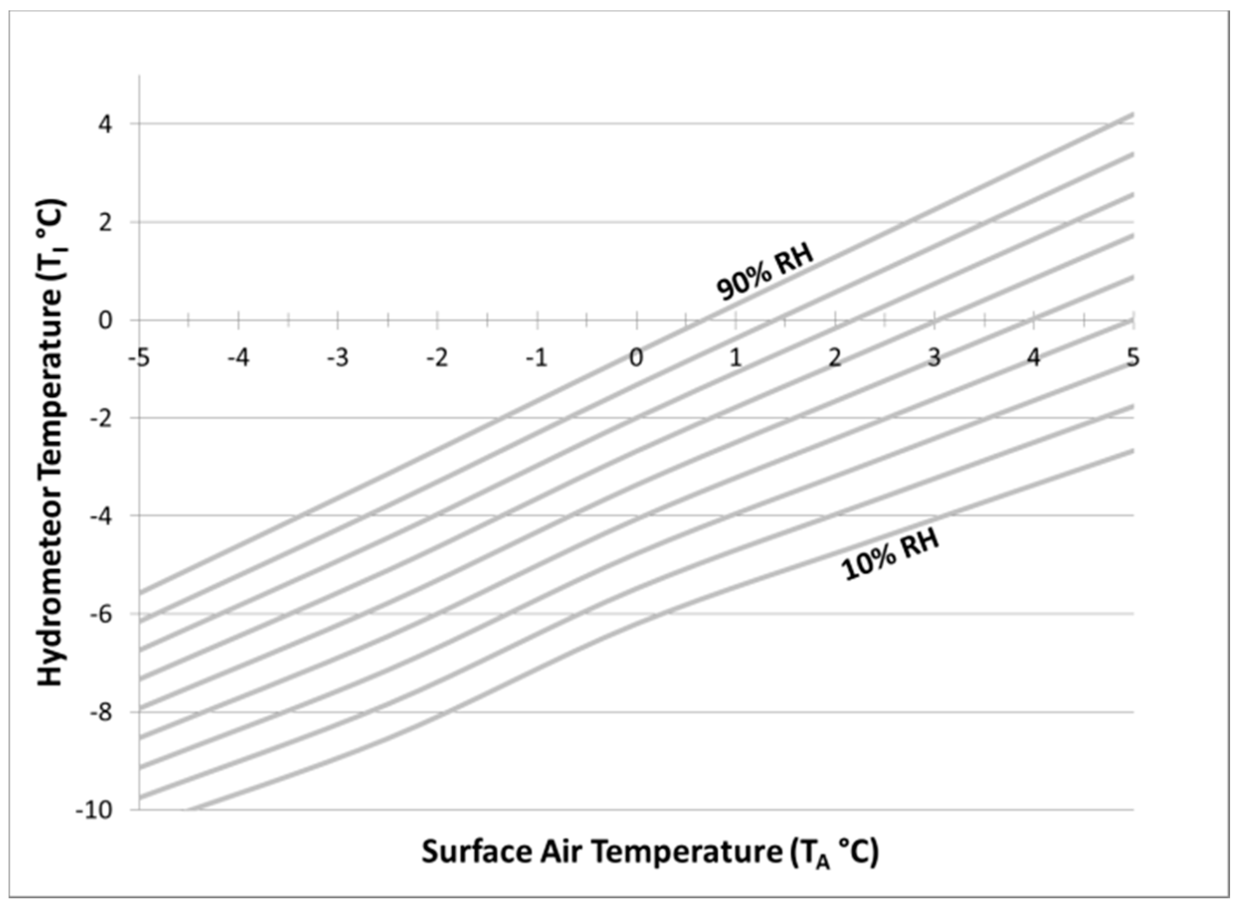
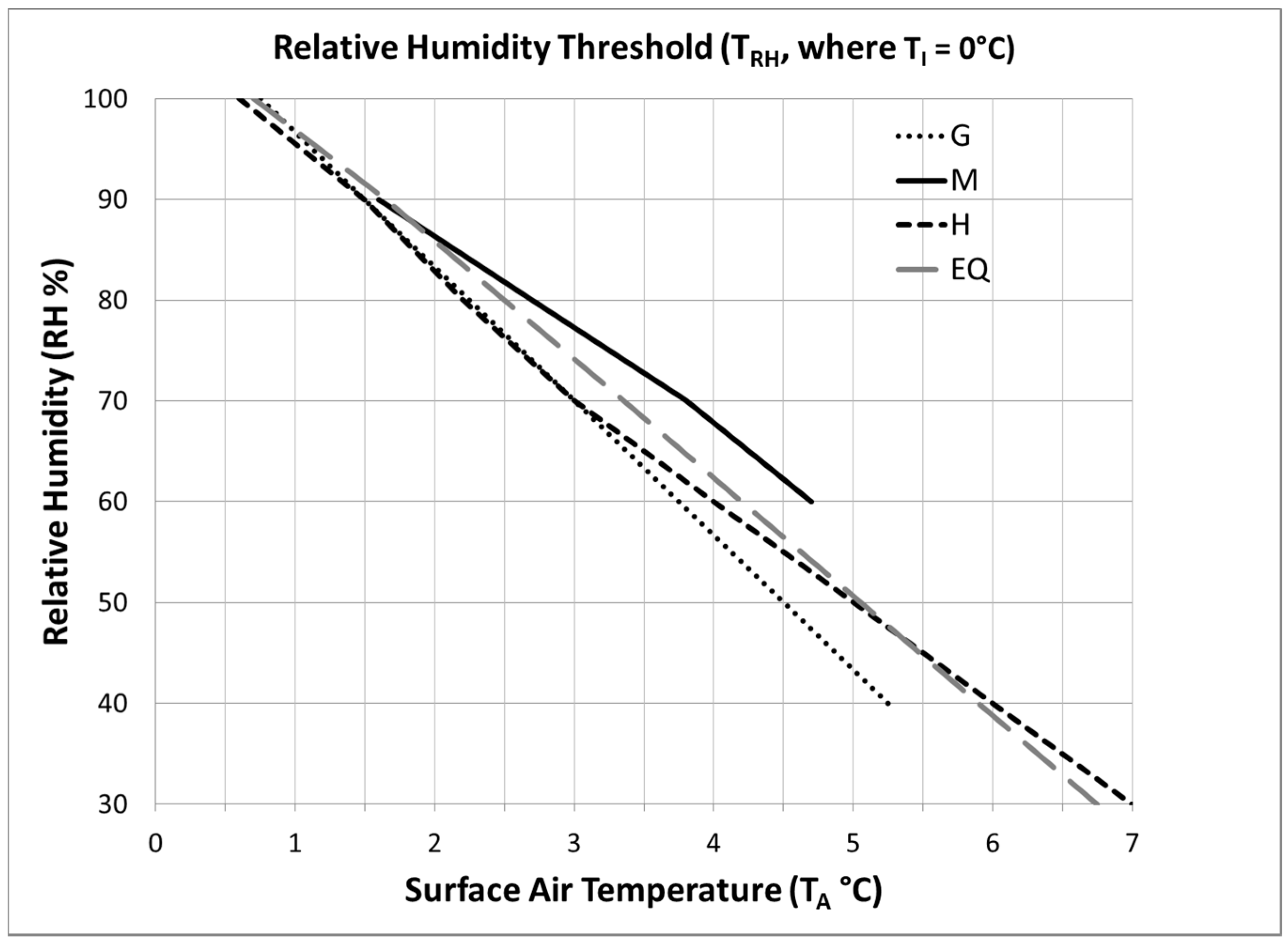
4.5. Temperature Schemes Including Humidity

PPDS can be based on different types of surface temperature. T_A methods do not include humidity, the second-most significant factor in determining precipitation type [27,29,33]. Some researchers have found T_D [20], T_W [27], and a combination of RH and T_A [1] to be better predictors of the precipitation phase. However, the assumption that surface humidity is fully representative of the atmospheric humidity is incorrect. It is crucial to remember that the atmosphere above the surface through which a hydrometeor falls is a major factor in melting and refreezing.

4.5.1. Dew Point Temperature Schemes

A T_D is the surface air temperature an air parcel would have to be cooled to in order to reach saturation at a constant pressure without moisture exchange [20]. Saturation temperatures differ between ice and water, therefore, requiring different formulas for T_D [29].

In near-saturated mountain environments, T_A ≈ T_D ≈ T_W and T_D was found to be more reliable for phase determination than T_A [20]. Marks et al. [20] hypothesized that in this moist environment, T_D was a proxy for hydrometeor temperature and would therefore identify the liquid or solid phase. Concerning this environment, a T_RS > 0 °C was found to misclassify more rain as snow than a threshold of T_D = 0 °C. Notably, this method did not work well when there was warm air aloft or when cloud bases were well above the surface [20].

T_D thresholds were found to have less spatial variations than T_RS [1,21]. No overall seasonal changes in T_D thresholds were found [1]. The T_D method can be easily applied when data is supplied by an AOS. However, knowledge of which relationship used by the AOS to derive T_D may be necessary.

4.5.2. Wet-Bulb Temperature Schemes

The T_W is the temperature an air parcel would be cooled to by evaporation until saturation without exchange of sensible heat [20]. A T_W scheme approximates the effect of sublimation and evaporation on snowflakes in air warmer and drier than the cloud in which it was formed [20,33]. T_W is derived from T_A, T_D, air pressure, and saturation vapor pressure. Snowfall frequently occurs when T_A > 0 °C and the near surface RH is < 100%, such that T_A > T_W > T_D [20]. Under these unsaturated (drier) conditions, T_W may be more effective than T_D in a PPDS [20].

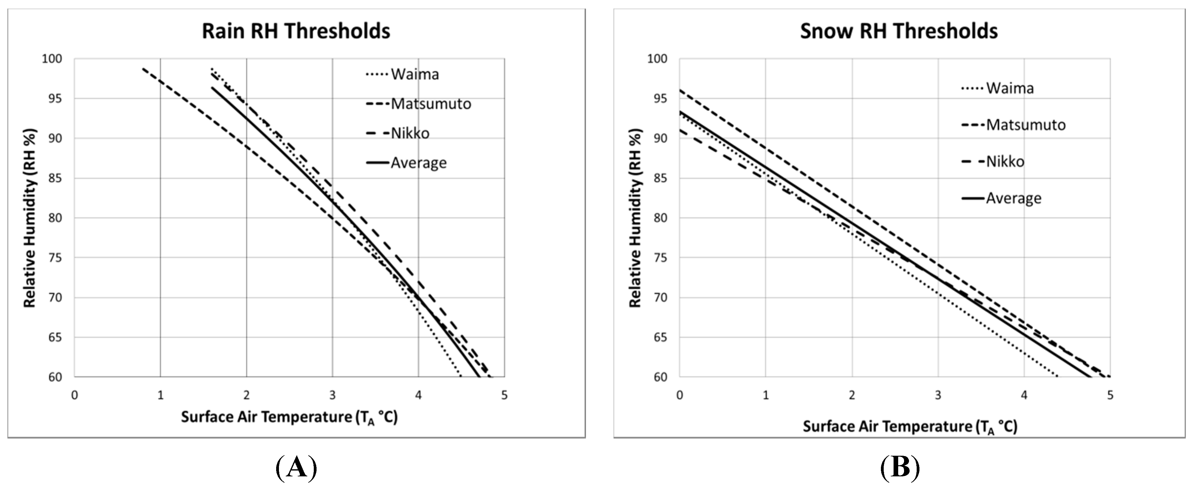
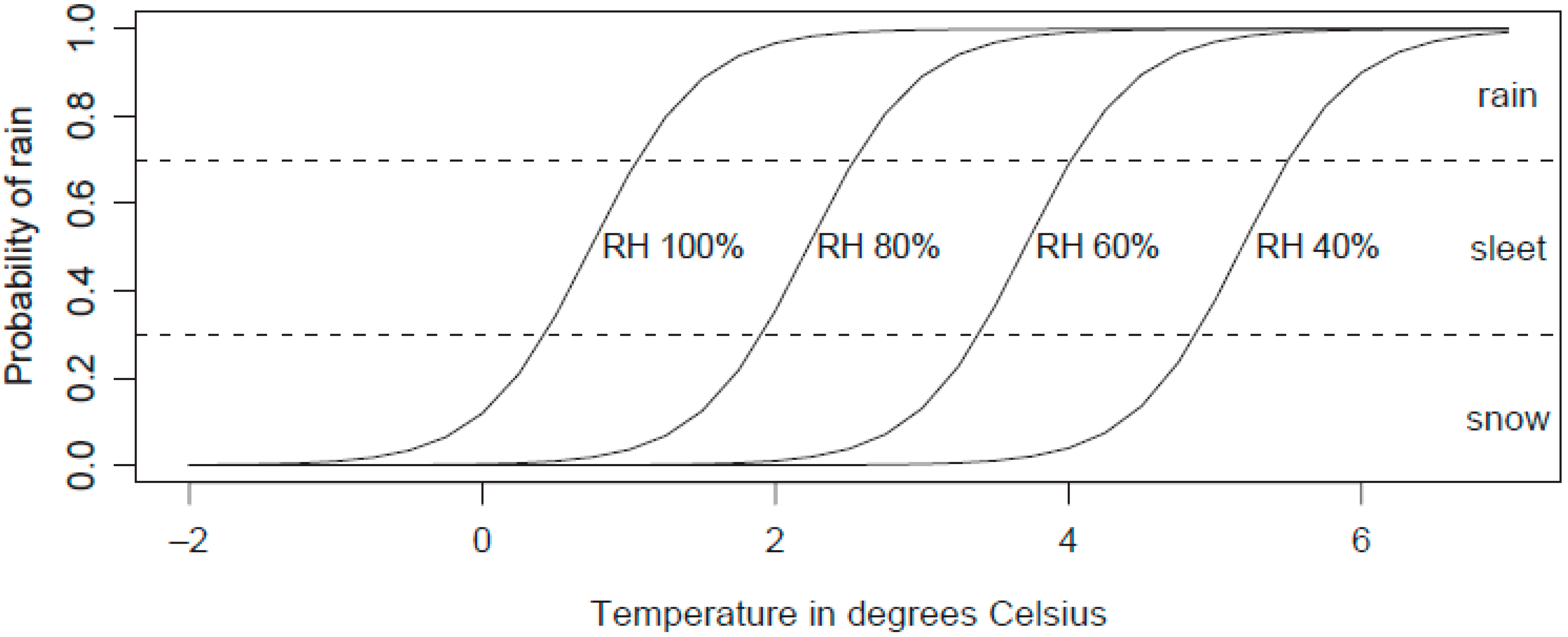
4.5.3. Relative Humidity Schemes

There are several studies showing that transition from rain to snow seems to take place at warmer temperatures for dry than for moist air [1,25,27,29,33,50]. Matsuo et al. [27] compared observed phase with surface T_A and RH in Japan to find snow and rain RH thresholds. All precipitation occurring for conditions plotted below the snow RH threshold were assumed snow, and above the rain RH threshold were assumed rain. Precipitation between the two RH thresholds was considered mixed. They found slightly varying relationships for different locations, but for each 10% drop in RH the T_RS would increase by about 1 °C (Figure 6A,B).

Figure 6. Rain (A) and snow (B) thresholds as a function of RH determined from equations in [27].

Figure 6. Rain (A) and snow (B) thresholds as a function of RH determined from equations in [27].

Similar trends were observed in Gjertsen and Ødegaard’s [33] study, where the probability of snow for a given T_A is increased with decreasing RH (Figure 7).

Harder and Pomeroy [29] utilized knowledge from research on sublimation of blowing snow to estimate a hydrometeor temperature (Ti) including the effects of RH. This Ti, achieved by an iterative process, was shown to be a better indicator of precipitation phase than T_RS. They used energy and mass balances of a sublimating ice sphere and assumed that the inner temperature of the ice sphere was the same as its surface temperature. They also assumed that the Nusselt and Sherwood numbers, indexes for the degree of turbulent transfer from a particle surface to the atmosphere of energy and water vapor respectively, were equal. Hydrometeor temperatures, calculated for different RH-values, using their relationships for the most interesting T_A range (−5 °C to + 5 °C) are shown in Figure 8, and confirm that Ti increases with RH.

Figure 7. Probability of rain versus surface air temperature for different RH (Figure 7 reprinted from Gjertsen and Ødegaard [33], with permission from Elsevier).

Figure 7. Probability of rain versus surface air temperature for different RH (Figure 7 reprinted from Gjertsen and Ødegaard [33], with permission from Elsevier).

Figure 8. Ti versus T_A with RH varying from 90% (top curve) to 10% (base curve).

Figure 8. Ti versus T_A with RH varying from 90% (top curve) to 10% (base curve).

An 80% increase in RH gives a Ti increase of ≈ 4.5 °C for T_A ≈ −5 °C and ≈ 6.5 °C for T_A ≈ +5 °C (Figure 8). The average Ti thus increases about 0.7 °C per 10% rise in RH in the relevant T_A range −5 to +5 °C. The hydrometeor rain/snow threshold temperature Ti = 0 °C, from now on denoted T_RH, thus occurs at 0.7 °C warmer T_A for each 10% drop in RH (Figure 8 and Figure 9). This agrees well with other reported T_RH relationships with about 0.85 °C warmer T_A for each 10% RH drop (Figure 9). The T_RH values from Gjertsen and Ødegaard [33], were determined by setting T_RH as the temperature having 50% SF and for Matsuo et al. [27] as the average of the reported rain and snow humidity thresholds (Figure 6A,B).

Figure 9. T_RH Relationship where T_I = 0 °C for a given T_A, and RH from studies; G = Gjertsen and Ødegaard [33], M = Matsuo et al. [27], H = Harder and Pomeroy [29], and EQ = Determined by Equation (1).

Figure 9. T_RH Relationship where T_I = 0 °C for a given T_A, and RH from studies; G = Gjertsen and Ødegaard [33], M = Matsuo et al. [27], H = Harder and Pomeroy [29], and EQ = Determined by Equation (1).

Since the T_RH relationships for T_A, and RH from all three studies show similar almost linear relationships (Figure 9) having about 0.85 °C warmer T_A per 10% RH decrease, the following simple relationship (for T_RH between 0 °C and 5 °C) is suggested;

T_RH = 0.75 + 0.085 × (100 − RH)

(1)

This very simple equation gives T_RS (40%) = 4.9 °C and T_RS (90%) = 1.65 °C, thus similar results as Matsuo et al. [27], Gjertsen and Ødegaard [33], and Harder and Pomeroy [29] (Figure 9). However, a weakness with RH–based methods is that RH is very sensitive to small errors in T_A, e.g., a 0.2 °C error leads to an RH error of 4% at T_A = 0 °C [65]. Accurate measurements of T_A are thus needed.

5. Summary

The goal here was to increase basic meteorological knowledge of precipitation phase change processes and to point out or identify techniques to improve surface based PPDS. Most hydrological models use daily average surface temperature based empirical formulas to imply precipitation phase without regard for atmospheric processes. These methods like all other surface based methods do not account for variations in atmospheric conditions that cause actual vertical temperature profiles to be uniquely modified by e.g., melting and refreezing.

However, methods developed or modified through knowledge of lower atmospheric interactions between air and hydrometers e.g., relative humidity, air mass boundaries, or precipitation intensity, should allow for statistically better chances of correct precipitation phase determination in surface based models. As a bonus, some of the below methods can be implemented without much difficulty since they only need AOS data already available in hydrological modeling.

Surface based precipitation phase determination methods can be improved by:

• Using a shorter a time-step:

Harder and Pomeroy [29], showed that by decreasing the time step from one day to one hour resulted in more than a 50% decrease in the temperature range for which mixed-phase (rain and/or snow) precipitation occurred.

This was most likely caused by many precipitation events occurring on a sub-daily timescale (most common exception warm frontal light stratiform precipitation) which often ranges from tens of minutes (intense cumuliform precipitation) to several hours in duration [48]. Since temperatures change diurnally with a maximum temperature in the afternoon and a minimum temperature in the morning, a decrease in the temperature sampling time step closer to the time scale to which precipitation events occur would result in a more representative temperature for precipitation phase determination.

• Introducing single (or dual rain/snow) thresholds which vary with relative humidity RH (%):

Matsuo et al. [27], Gjertsen and Ødegaard [33], and Harder and Pomeroy [29] all show that T_RS increases with decreasing RH. Based on these studies, it is shown that, for the surface air temperature range of 0 °C to 5 °C, T_RH could be approximated by 0.75 + 0.085 × (100 − RH).

• Identification of air mass boundaries:

Feiccabrino et al. [48] found T_S and T_R values for a group of cold air mass boundaries to be 1 °C warmer than that of all other observations. When these observation groups were analyzed separately, total misclassified precipitation was reduced by 23% in the temperature range −1 to 5 °C.

This was thought to be the cause of warm air rising over a lower denser cold air mass for most precipitation events with the main exception being cold fronts having precipitation occur ahead of the front in a single air mass. This theory worked in a Central United States continental climate [48] but did not improve precipitation phase identification in the maritime mountain environment of the Scandinavian Peninsula [19]. In a maritime or island environment surface air in the winter is modified by the warm ocean temperatures making all but the strongest frontal passages advect warm air over the land. This ocean affect could be the reason for such different results between studies.

• Inclusion of precipitation intensity and/or duration:

No direct study available for confirmation, but Harder and Pomeroy [29] noted that the temperature range between T_S and T_R narrowed for heavy precipitation events and Minder et al. [17] showed an increase in the isothermal layer depth associated with melting precipitation. The presence of unstable air under the isothermal layer should allow for snow reaching the ground at warmer air temperatures similar to ocean effects from Ólafsson and Haraldsdóttir [30].

The lack of a study in this area would suggest that either negative results were found and therefore not published, or it has not been looked into. Considering that most studies are carried out using a daily or hourly precipitation and temperature time-step, it is possible that cooling of the temperature due to melting and sublimation occurred rapidly enough to keep warm high intensity snow events from being observed often enough to be a notable issue. The isothermal layer can thicken for long duration events (Section 2.2.3), but the surface temperature can also lower with sublimation, evaporation, or, to a lesser extent, modify to being closer to the precipitation temperature.

• Seasonal and/or terrain dependent lapse rates:

Dai [18] reported a warm bias (+0.7 °C) for T_RS over oceans compared to over land. This phenomena was confirmed in two other studies [19,30], and is thought to be caused by the ocean heating the near surface atmosphere resulting in higher lapse rates over the coast and water.

It is therefore suggested and shown [19] that different snow/rain temperature threshold values should be used for different geographic landscapes. This is due to ocean/water heating the near surface air causing the snow/rain threshold to be warmer over open water than land. The rain/snow threshold differences on land could be caused by terrain effects on cloud formation and precipitation intensity.

This paper was directed mostly towards techniques to improve point precipitation phase identification for possible quality assurance checks, reanalysis of historical data, or the assigning of a precipitation phase when there is no manual observation or automated device present to report a phase. Many of the automated methods/instruments that report precipitation phase use; (1) Doppler radar; (2) optical sensors [66]; (3) hotplates [67] or (4) two dimensional video distrometers (2DVD) [68]. However, they have often been put into operation without an in-depth intercomparison which brings into question the quality, consistency, compatibility, and representativeness of their data [66]. In response to this, the WMO (World Meteorological Organization) Solid Precipitation InterComparison (WMO-SPICE) study was created. The initial WMO-SPICE findings are just now becoming available e.g., [69,70].

It is also beyond the scope of this paper, however of great value to understand how landscapes such as forest or open fields affect the spatial distribution of snowfall, see e.g., [71].

6. Conclusions

Fixed rain/snow thresholds in surface based models tend to integrate average atmospheric conditions that control phase change when distinction could be useful. Distinct Atmospheric conditions and terrain features which cause warmer than normal rain/snow temperature thresholds are:

• Cold frontal passage
• Locations over or near large ice free water bodies
• Low relative humidity
• Long duration or high intensity precipitation events
• Locations on the windward side of mountains (caused by increased precipitation intensity)

The above surface and atmospheric weather conditions could all be identified using surface observations while the above terrain features that interact with lower atmospheric conditions can be easily identified on topographic maps. This information is readily available and should therefore be used to improve precipitation phase determination in surface based models.

References

1. Ye, H.; Cohen, J.; Rawlins, M. Discrimination of solid from liquid precipitation over northern Eurasia using surface atmospheric conditions. J. Hydrometeorol. 2013, 14, 1345–1355. [Google Scholar] [CrossRef]
2. Wen, L.; Nagabhatla, N.; Lü, S.; Wang, S.Y. Impact of rain snow threshold temperature on snow depth simulation in land surface and regional atmospheric models. Adv. Atmos. Sci. 2013, 30, 1449–1460. [Google Scholar] [CrossRef]
3. Thériault, J.M.; Rasmussen, R.; Ikeda, K.; Landolt, S. Dependence of snow gauge collection efficiency on snowflake characteristics. J. Appl. Meteorol. Climatol. 2012, 51, 745–762. [Google Scholar] [CrossRef]
4. Bartlett, P.A.; MacKay, M.D.; Verseghy, D.L. Modified snow algorithms in the Canadian land surface scheme: Model runs and sensitivity analysis at three Boreal forest stands. Atmos. Ocean 2006, 43, 207–222. [Google Scholar] [CrossRef]
5. Coudrain, A.; Francou, B.; Kundzewicz, Z.W. Glacier shrinkage in the Andes and consequences for water resources—Editorial. Hydrol. Sci. J. 2005, 50, 925–932. [Google Scholar]
6. Lundberg, A.; Fieccabrino, J. Sea ice growth, modeling of precipitation phase. In Proceedings of the 20th International Conference on Port and Ocean Engineering under Arctic Conditions, Lulea, Sweden, 9–12 June 2009.
7. Davis, R.E.; Lowit, M.B.; Knappenberger, P.C.; Legates, D.R. A climatology of snowfall-temperature relationships in Canada. J. Geophys. Res. Atmos. 1999, 104, 11985–11994. [Google Scholar] [CrossRef]
8. Bellaire, S.; Jamieson, B. Forecasting the formation of critical snow layers using a coupled snow cover and weather model. Cold Reg. Sci. Technol. 2013, 94, 37–44. [Google Scholar] [CrossRef]
9. Lundberg, A.; Nakai, Y.; Thunehed, H.; Halldin, S. Snow accumulation in forests from ground and remote-sensing data. Hydrol. Process. 2004, 18, 1941–1955. [Google Scholar] [CrossRef]
10. Lundberg, A.; Feiccabrino, J.; Westerlund, C.; Al-Ansari, N. Urban snow deposits versus snow cooling plants in northern Sweden: A quantitative analysis of snow melt pollutant releases. Water Qual. Res. J. Can. 2014, 49, 32–42. [Google Scholar] [CrossRef]
11. Stewart, T.R.; Pielke, R., Jr.; Nath, R. Understanding user decision making and the value of improved precipitation forecasts lessons from a case study. Bull. Am. Meteorol. Soc. 2004, 85, 223–235. [Google Scholar] [CrossRef]
12. Gray, D.M.; Toth, B.; Zhao, L.; Pomeroy, J.W.; Granger, R.J. Estimating areal snowmelt infiltration into frozen soils. Hydrol. Process. 2001, 15, 3095–3111. [Google Scholar] [CrossRef]
13. Ecke, F.; Christensen, P.; Rentz, R.; Nilsson, M.; Sandström, P.; Hörnfeldt, B. Landscape structure and the long-term decline of cyclic grey-sided voles in Fennoscandia. Landsc. Ecol. 2010, 25, 551–560. [Google Scholar] [CrossRef]
14. Braun, L.N. Modeling of the snow-water equivalent in the mountain environment. In Snow in Hydrology and Forests in High Alpine Areas; Bergmann, H., Lang, H., Frey, W., Issler, D., Salm, B., Eds.; IAHS Press: Wallingford, UK, 1991; pp. 3–17. [Google Scholar]
15. Sivapalan, M.; Takeuchi, K.; Franks, S.W.; Gupta, V.K.; Karambiri, H.; Lakshmi, V.; Liang, X.; McDonnell, J.J.; Mendiondo, E.M.; O’Connell, P.E.; et al. IAHS decade on Predictions in Ungauged Basins (PUB), 2003–2012: Shaping an exciting future for the hydrological sciences. Hydrol. Sci. J. 2003, 48, 857–880. [Google Scholar] [CrossRef]
16. Fang, X.; Pomeroy, J.W.; Ellis, C.R.; MacDonald, M.K.; DeBeer, C.M.; Brown, T. Multi-variable evaluation of hydrological model predictions for a headwater basin in the Canadian Rocky Mountains. Hydrol. Earth Syst. Sci. 2013, 17, 1635–1659. [Google Scholar] [CrossRef]
17. Minder, J.R.; Durran, D.R.; Roe, G.H. Mesoscale controls on the mountainside snow line. J. Atmos. Sci. 2011, 68, 2107–2127. [Google Scholar] [CrossRef]
18. Dai, A. Temperature and pressure dependence of the rain-snow phase transition over land and ocean. Geophys. Res. Lett. 2008. [Google Scholar] [CrossRef]
19. Feiccabrino, J. A cross sectional study of rain/snow threshold changes from the North Sea across the Scandinavian Mountains to the Bay of Bothnia. In Proceedings of the 20th International Northern Research Basins Symposium and Workshop, Kuusamo, Finland, 16–21 August 2015; pp. 4–13.
20. Marks, D.; Winstral, A.; Reba, M.; Pomeroy, J.; Kumar, M. An evaluation of methods for determining during-storm precipitation phase and the rain/snow transition elevation at the surface in a mountain basin. Adv. Water Resour. 2013, 55, 98–110. [Google Scholar] [CrossRef]
21. Feiccabrino, J.; Gustafsson, D.; Lundberg, A. Surface-based precipitation phase determination methods in hydrological models. Hydrol. Res. 2013, 44, 44–57. [Google Scholar] [CrossRef]
22. Kongoli, C.E.; Bland, W.L. Long-term snow depth simulations using a modified atmosphere-land exchange model. Agric. For. Meteorol. 2000, 104, 273–287. [Google Scholar] [CrossRef]
23. United States Army Corps of Engineers (USACE). Snow Hydrology: Summary Report of the Snow Investigations; United States Army Corps of Engineers North Pacific Division: Portland, OR, USA, 1956; p. 437. [Google Scholar]
24. Kane, D.L.; Stuefer, S. Reflecting on the status of precipitation data collection in Alaska: A case study. Hydrol. Res. 2015, 46, 478–493. [Google Scholar] [CrossRef]
25. Stewart, R.E. Precipitation types in the transition region of winter storms. Bull. Am. Meteorol. Soc. 1992, 73, 287–296. [Google Scholar] [CrossRef]
26. Thériault, J.M.; Stewart, R.E. A parameterization of the microphysical processes forming many types of winter precipitation. J. Atmos. Sci. 2010, 67, 1492–1508. [Google Scholar] [CrossRef]
27. Matsuo, T.; Sato, Y.; Sasyo, Y. Relationship between types of precipitation on the ground and surface meteorological elements. J. Meteorol. Soc. Jpn. 1981, 59, 462–475. [Google Scholar]
28. Lundquist, J.D.; Neiman, P.J.; Martner, B.; White, A.B.; Gottas, J.D.; Ralph, F.M. Rain versus snow in the Sierra Nevada, California: Comparing Doppler profiling radar and surface observations of melting level. J. Hydrometeorol. 2008, 9, 194–211. [Google Scholar] [CrossRef]
29. Harder, P.; Pomeroy, J. Estimating precipitation phase using a psychrometric energy balance method. Hydrol. Process. 2013, 27, 1901–1914. [Google Scholar] [CrossRef]
30. Ólafsson, H.; Haraldsdóttir, S.H. Diurnal, seasonal, and geographical variability of air temperature limits of snow and rain. In Proceedings of the International Conference on Alpine Meteorology (ICAM 2003), Brig, Switzerland, 19–23 May 2003; pp. 473–476.
31. Kienzle, S.W. A new temperature based method to separate rain and snow. Hydrol. Process. 2008, 22, 5067–5085. [Google Scholar] [CrossRef]
32. Fassnacht, S.R.; Kouwen, N.; Soulis, E.D. Surface temperature adjustments to improve weather radar representation of multi-temporal winter precipitation accumulations. J. Hydrol. 2001, 253, 148–168. [Google Scholar] [CrossRef]
33. Gjertsen, U.; Ødegaard, V. The water phase of precipitation—A comparison between observed, estimated and predicted values. Atmos. Res. 2005, 77, 218–231. [Google Scholar] [CrossRef]
34. Davison, B. Snow Accumulation in a Distributed Hydrological Model. Ph.D. Thesis, University of Waterloo, Waterloo, ON, Canada, 2003. [Google Scholar]
35. NOAA National Weather Service Radiosonde Observations. Available online: http://www.ua.nws.noaa.gov/factsheet.htm (accessed on 23 September 2015).
36. Kain, J.S.; Goss, S.M.; Baldwin, M.E. The melting effect as a factor in precipitation-type forecasting. Weather Forecast 2000, 15, 700–714. [Google Scholar] [CrossRef]
37. Fujibe, F. On the near-0 °C frequency maximum in surface air temperature under precipitation: A statistical evidence for the melting effect. J. Meteorol. Soc. Jpn. 2001, 79, 731–739. [Google Scholar] [CrossRef]
38. Lackmann, G.M.; Keeter, K.; Lee, L.G.; Ek, M.B. Model representation of freezing and melting precipitation: Implications for winter weather forecasting. Weather Forecast 2002, 17, 1016–1033. [Google Scholar] [CrossRef]
39. Mitra, S.K.; Vohl, O.; Ahr, M.; Pruppacher, H.R. A wind tunnel and theoretical study of the melting behavior of atmospheric ice particles IV: Experiment and theory for snowflakes. J. Atmos. Sci. 1990, 47, 584–591. [Google Scholar] [CrossRef]
40. Chen, S.H.; Sun, W.Y. A one-dimensional time dependent cloud model. J. Meteorol. Soc. Jpn. 2002, 80, 99–118. [Google Scholar] [CrossRef]
41. Hong, S.Y.; Lim, J.O.J. The WRF single-moment 6-class microphysics scheme (WSM6). J. Korean Meteorol. Soc. 2006, 42, 129–151. [Google Scholar]
42. Skamarock, W.C.; Klemp, J.B.; Dudhia, J.; Gill, D.O.; Barker, D.M.; Duda, M.G.; Huang, X.Y.; Wang, W.; Powers, J.G. A Description of the Advanced Research WRF Version 3; NCAR Tech. Note. NCAR/TN-475+ STR; National Center for Atmospheric Research: Boulder, CO, USA, 2008. [Google Scholar]
43. Venne, M.G.; Jasperson, W.H.; Venne, D.E. Difficult Weather: A Review of Thunderstorms, Fog, and Stratus, and Winter Precipitation Forecasting; AIRFM Command Tech. Report #A246633; Augsburg Coll Minneapolis MN Center for Atmospheric and Space Sciences: Minneapolis, MN, USA, 1997. [Google Scholar]
44. McNulty, R.P. Winter Precipitation Type; NWS Central Region Tech. Attach. 88–4; National Weather Service: Kansas City, MO, USA, 1988.
45. Ruddell, A.R.; Budd, W.F.; Smith, I.N.; Keage, P.L.; Jones, R. The South East Australian Alpine Climate Study: A report by the Meteorology Department, University of Melbourne, for the Alpine Resorts Commissions; Department of Meteorology, University of Melbourne: Melbourne, Australia, 1990; p. 115. [Google Scholar]
46. Schreider, S.Y.; Whetton, P.H.; Jakeman, A.J.; Pittock, A.B. Runoff modelling for snow-affected catchments in the Australian alpine region, eastern Victoria. J. Hydrol. 1997, 200, 1–23. [Google Scholar] [CrossRef]
47. Sælthun, N.R. “The Nordic” HBV Model, Description and Documentation of the Model Version Developed for the Project ‘Climate Change and Energy Production’; Norwegian Water Resources and Energy Administration (NVE): Oslo, Norway, 1996. [Google Scholar]
48. Feiccabrino, J.; Lundberg, A.; Gustafsson, D. Improving surface-based precipitation phase determination through air mass boundary identification. Hydrol. Res. 2012, 43, 179–191. [Google Scholar]
49. Yang, Z.L.; Dickinson, R.E.; Robock, A.; Vinnikov, K.Y. Validation of the snow submodel of the biosphere-atmosphere transfer scheme with Russian snow cover and meteorological observational data. J. Clim. 1997, 10, 353–373. [Google Scholar] [CrossRef]
50. Motoyama, H. Simulation of seasonal snowcover based on air temperature and precipitation. J. Appl. Meteorol. 1990, 29, 1104–1110. [Google Scholar] [CrossRef]
51. L’hôte, Y.; Chevallier, P.; Coudrain, A.; Lejeune, Y.; Etchevers, P. Relationship between precipitation phase and air temperature: Comparison between the Bolivian Andes and the Swiss Alps. Hydrol. Sci. J. 2005, 50, 989–997. [Google Scholar]
52. Braun, L.N.; Lang, H. Simulation of snowmelt runoff in lowland and lower alpine regions of Switzerland. In Proceedings of the Budapest Symposium, Budapest, Hungary, 2–10 July 1986; pp. 125–140.
53. Hottelet, C.; Blažková, Š.; Blčík, M. Application of the ETH snow model to three basins of different character in Central Europe. Nord. Hydrol. 1994, 25, 113–128. [Google Scholar]
54. Zhang, Y.; Wang, S.; Barr, A.G.; Black, T.A. Impact of snow cover on soil temperature and its simulation in a boreal aspen forest. Cold Reg. Sci. Technol. 2008, 52, 355–370. [Google Scholar] [CrossRef]
55. Caballero, Y.; Chevallier, P.; Gallaire, R.; Pillco, R. Flow modelling in a high mountain valley equipped with hydropower plants: Rio Zongo Valley, Cordillera Real, Bolivia. Hydrol. Process. 2004, 18, 939–957. [Google Scholar] [CrossRef]
56. Baun, S.D. Frequency Mapping of Maximum Snow Water Equivalent of March Snow Cover over Minnesota and the Eastern Dakotas; NWS Central Region Tech. Memo. CR-113; National Weather Service: Silver Spring, MD, USA, 1998.
57. Pomeroy, J.W.; Gray, D.M.; Brown, T.; Hedstrom, N.R.; Quinton, W.L.; Granger, R.J.; Carey, S.K. The cold regions hydrological model: A platform for basing process representation and model structure on physical evidence. Hydrol. Process. 2007, 21, 2650–2667. [Google Scholar] [CrossRef]
58. Daly, S.F.; Davis, R.; Ochs, E.; Pangburn, T. An approach to spatially distributed snow modelling of the Sacramento and San Joaquin basins, California. Hydrol. Process. 2000, 14, 3257–3271. [Google Scholar] [CrossRef]
59. Auer, A.H., Jr. The rain versus snow threshold temperatures. Weatherwise 1974. [Google Scholar] [CrossRef]
60. Bjerknes, J. On the structure of moving cyclones. Mon. Weather Rev. 1919, 47, 95–99. [Google Scholar] [CrossRef]
61. Oliver, V.J.; Oliver, M.B. Weather analysis from single-station data. In Handbook of Meteorology; Berry, F.A., Bolay, E., Beers, N.R., Eds.; McGraw-Hill Book Co.: New York, NY, USA, 1945; pp. 858–879. [Google Scholar]
62. Fraedrich, K.; Bach, R.; Naujokat, N. Single station climatology of central European fronts Number, time and precipitation statistics. Beitr. Phys. Atmos. 1986, 59, 54–65. [Google Scholar]
63. Sanders, F. A proposed method of surface map analysis. Mon. Weather Rev. 1999, 127, 945–955. [Google Scholar] [CrossRef]
64. Schultz, D.M. A review of cold fronts with prefrontal troughs and wind shifts. Mon. Weather Rev. 2005, 133, 2449–2472. [Google Scholar] [CrossRef]
65. Lundberg, A.; Halldin, S. Evaporation of intercepted snow: Analysis of governing factors. Water Resour. Res. 1994, 30, 2587–2598. [Google Scholar] [CrossRef]
66. Nuti, R.; Wong, K. Instruments and Observing Methods; WMO/TD-No.1544; World Meteorological Organization: Geneva, Switzerland, 2010. [Google Scholar]
67. Boudala, F.S.; Rasmussen, R.; Isaac, G.A.; Scott, B. Performance of hot plate for measuring solid precipitation in complex terrain during the 2010 Vancouver Winter Olympics. J. Atmos. Ocean. Technol. 2014, 31, 437–446. [Google Scholar] [CrossRef]
68. Grazioli, J.; Tuia, D.; Monhart, S.; Schneebeli, M.; Raupach, T.; Berne, A. Hydrometeor classification from two dimensional video disdrometer data. Atmos. Meas. Tech. 2014, 7, 2869–2882. [Google Scholar] [CrossRef]
69. Thériault, J.M.; Rasmussen, R.; Petro, E.; Trépanier, J.Y.; Colli, M.; Lanza, L.G. Impact of Wind Direction, Wind Speed, and Particle Characteristics on the Collection Efficiency of the Double Fence Intercomparison Reference. J. Appl. Meteorol. Climatol. 2015, 54, 1918–1930. [Google Scholar] [CrossRef]
70. Yang, D. Double fence intercomparison reference DFIR vs bush gauge for “true” snowfall measurement. J. Hydrol. 2014, 509, 94–100. [Google Scholar] [CrossRef]
71. Garvelmann, J.; Pohl, S.; Weiler, M. From observation to the quantification of snow processes with a time-lapse camera network. Hydrol. Earth Syst. Sci. 2013, 17, 1415–1429. [Google Scholar] [CrossRef]