
A Hydrological Concept including Lateral Water Flow Compatible with the Biogeochemical Model ForSAFE

Abstract
:1. Introduction
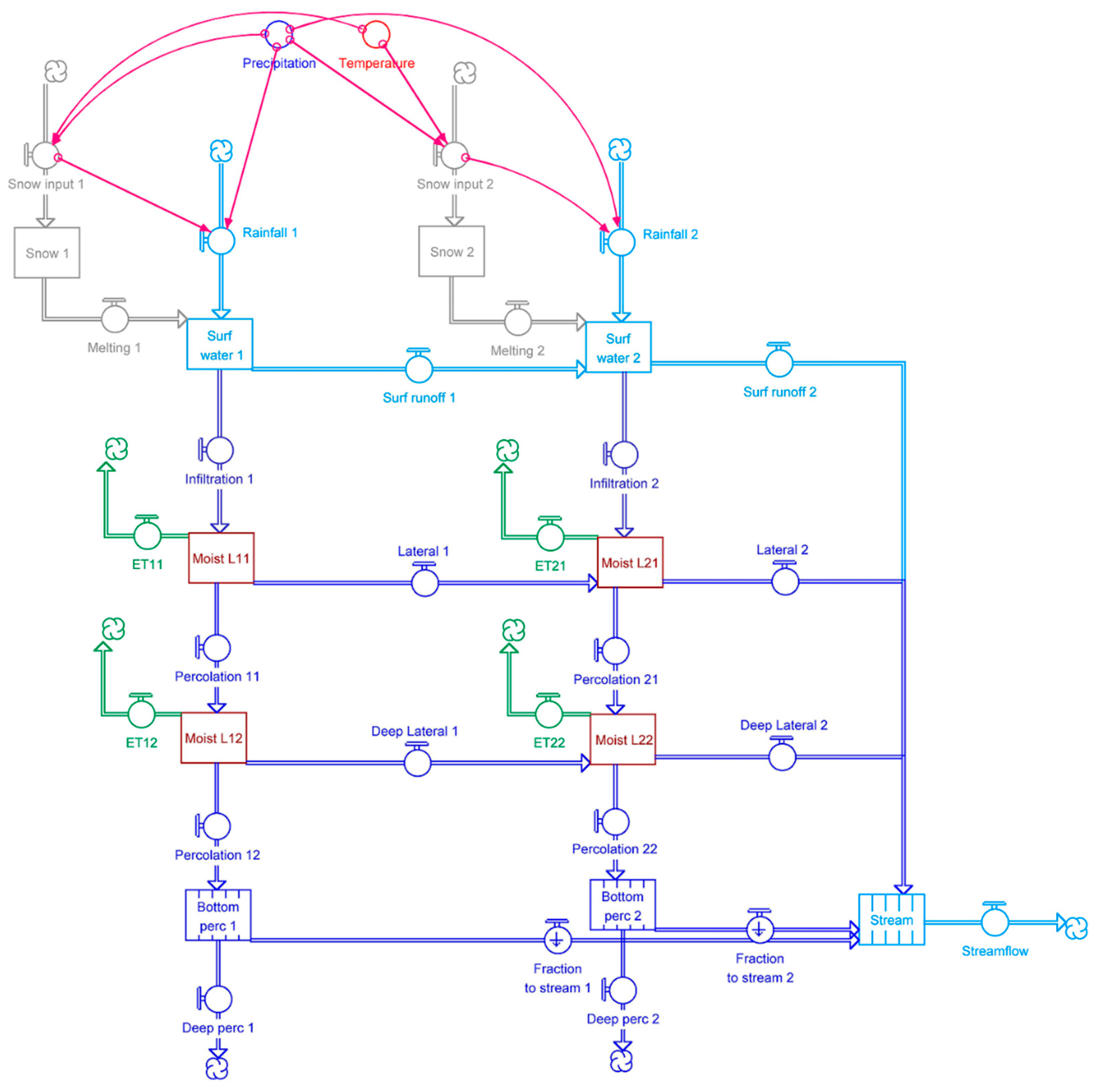
2. Model Description
- -
- increased time resolution from monthly to daily time steps
- -
- the water flow from a given soil layer is constrained by the amount of water that receiving layers can accept vertically and horizontally
- -
- the water flow is given a velocity regulated by the soil conductivity, controlling the amount of water that can move within each time step (per day)
- -
- inclusion of water movement along a slope, i.e., surface runoff and lateral flow
- -
- the soil hydraulic properties are assessed as a function of soil texture
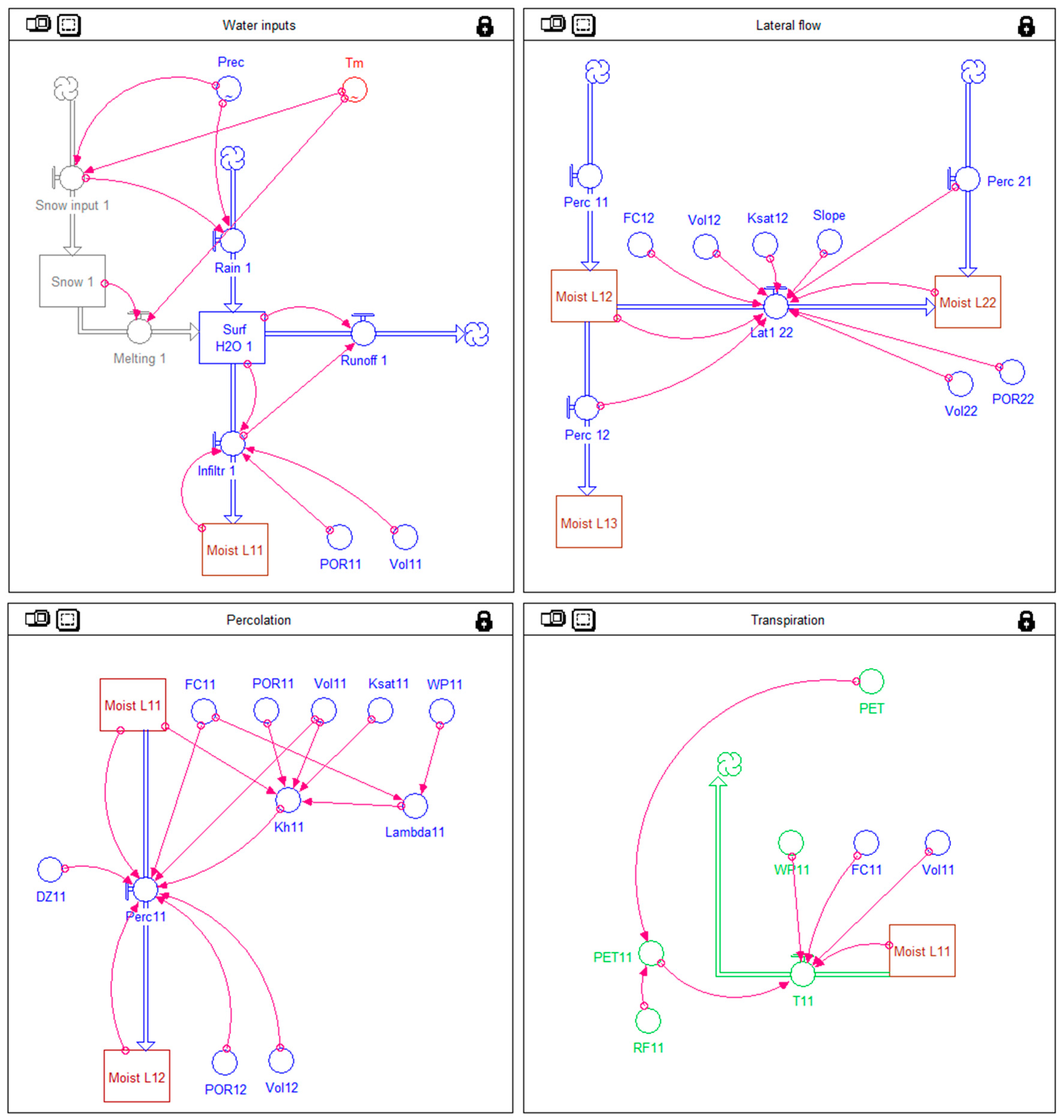
2.1. Water Inputs to the Soil
2.2. Water outputs from the soil
- Percolation
- Lateral flow
- Transpiration
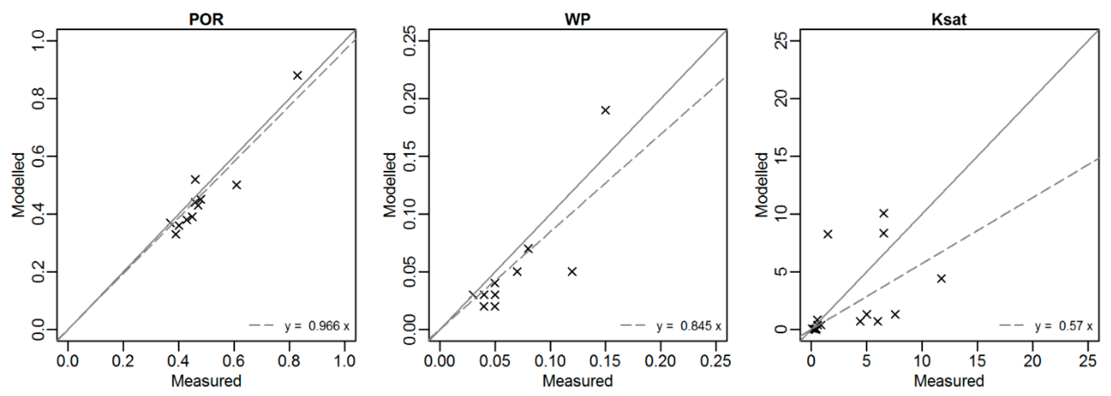
- the porosity, the fraction of pores in the soil volume (POR, m3 water m−3 soil)
- the field capacity, the water content held in the soil when free drainage by gravity has stopped (FC, m3 water m−3 soil)
- the permanent wilting point, the soil moisture content at which plants cannot extract more water from the soil (WP, m3 water m−3 soil)
- the saturated hydraulic conductivity, the rate at which water moves through the pores in the saturated soil (Ksat, m·d−1)
- the unsaturated hydraulic conductivity, the rate at which water moves through the pores in the unsaturated soil (Kh, m·d−1)
- the slope of the soil moisture characteristic, which is the relation between water tension and volumetric water content (λ)
2.2.1. Percolation
2.2.2. Lateral Water Flow
2.2.3. Transpiration
3. Model Test
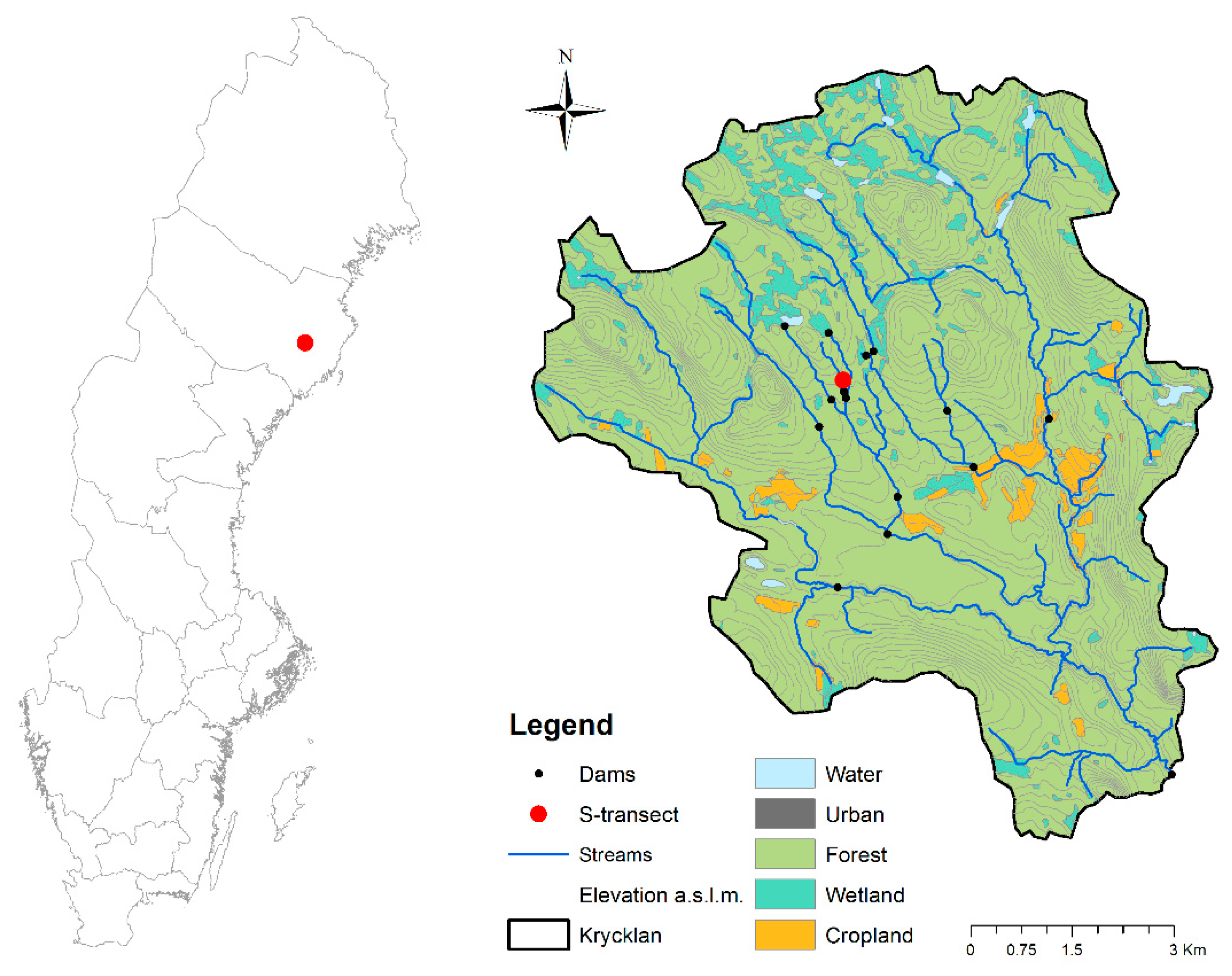
3.1. Site Description
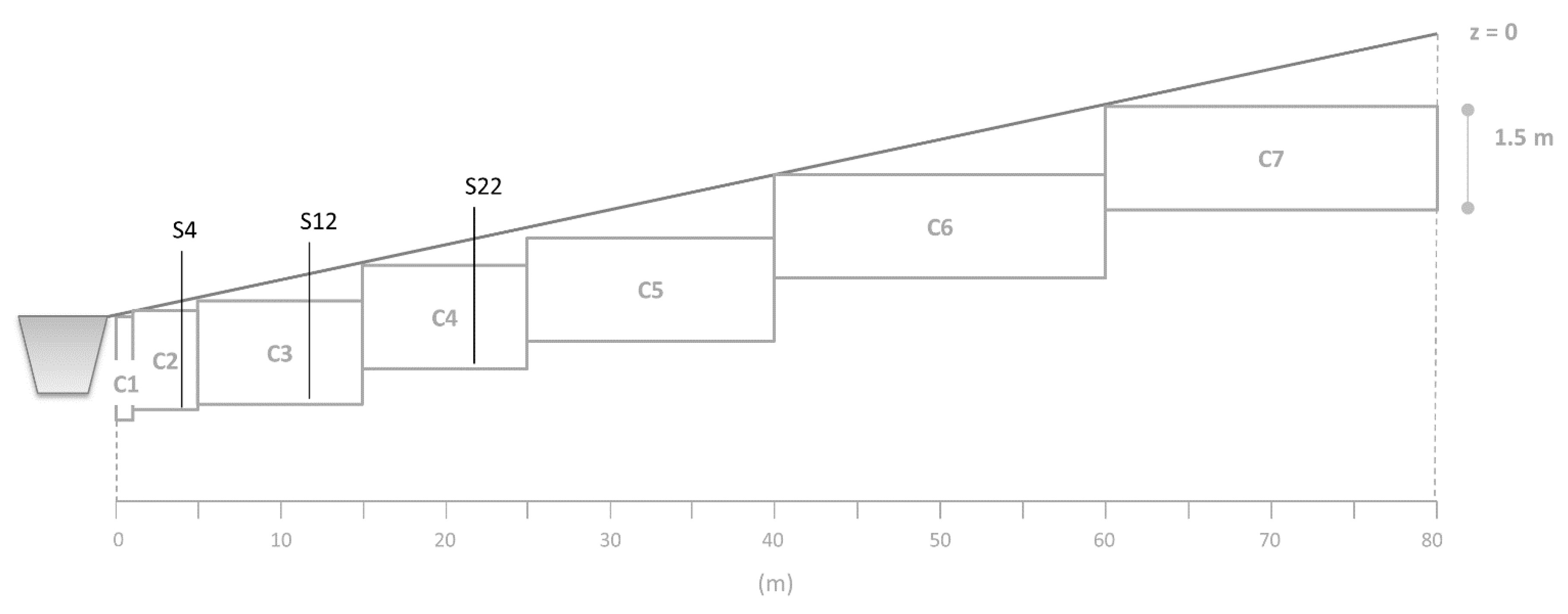
3.2. Transect Model
3.3. Parameterization of Soil Hydraulic Properties
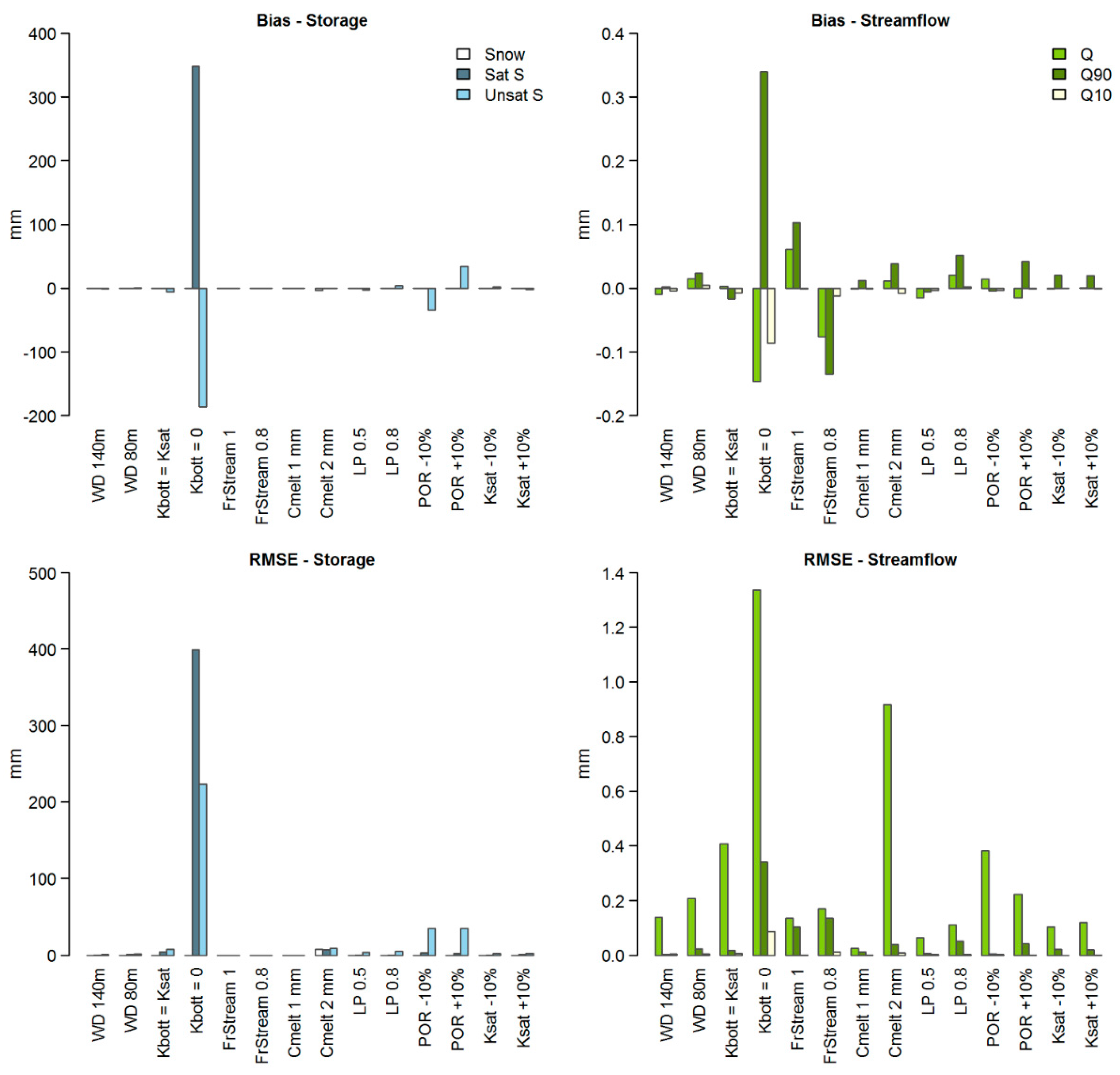
3.4. Sensitivity Analysis
- -
- the fraction of bottom percolation to the stream (FrStream): when increased the overall streamflow increases, as indicated by the Bias;
- -
- an increase of snow melting factor (Cmelt) affects significantly the distribution of the flow during the year (increase of RMSE), but has a minor effect on the overall water balance.
3.5. Calibration
4. Model Results and Discussion
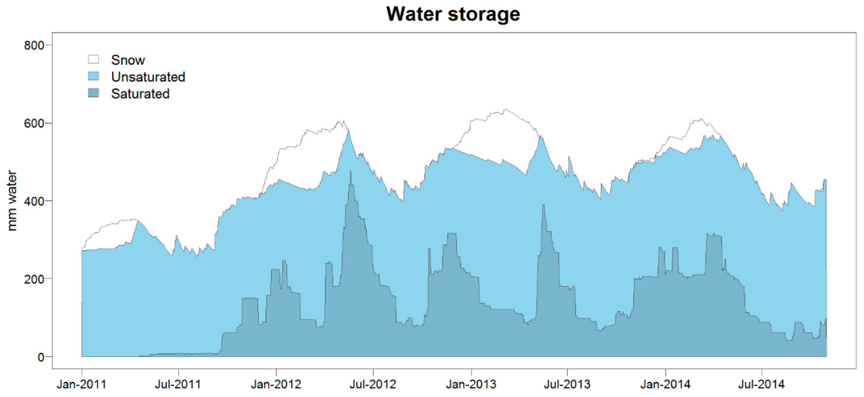
4.1. Simulated Water Storage and Fluxes
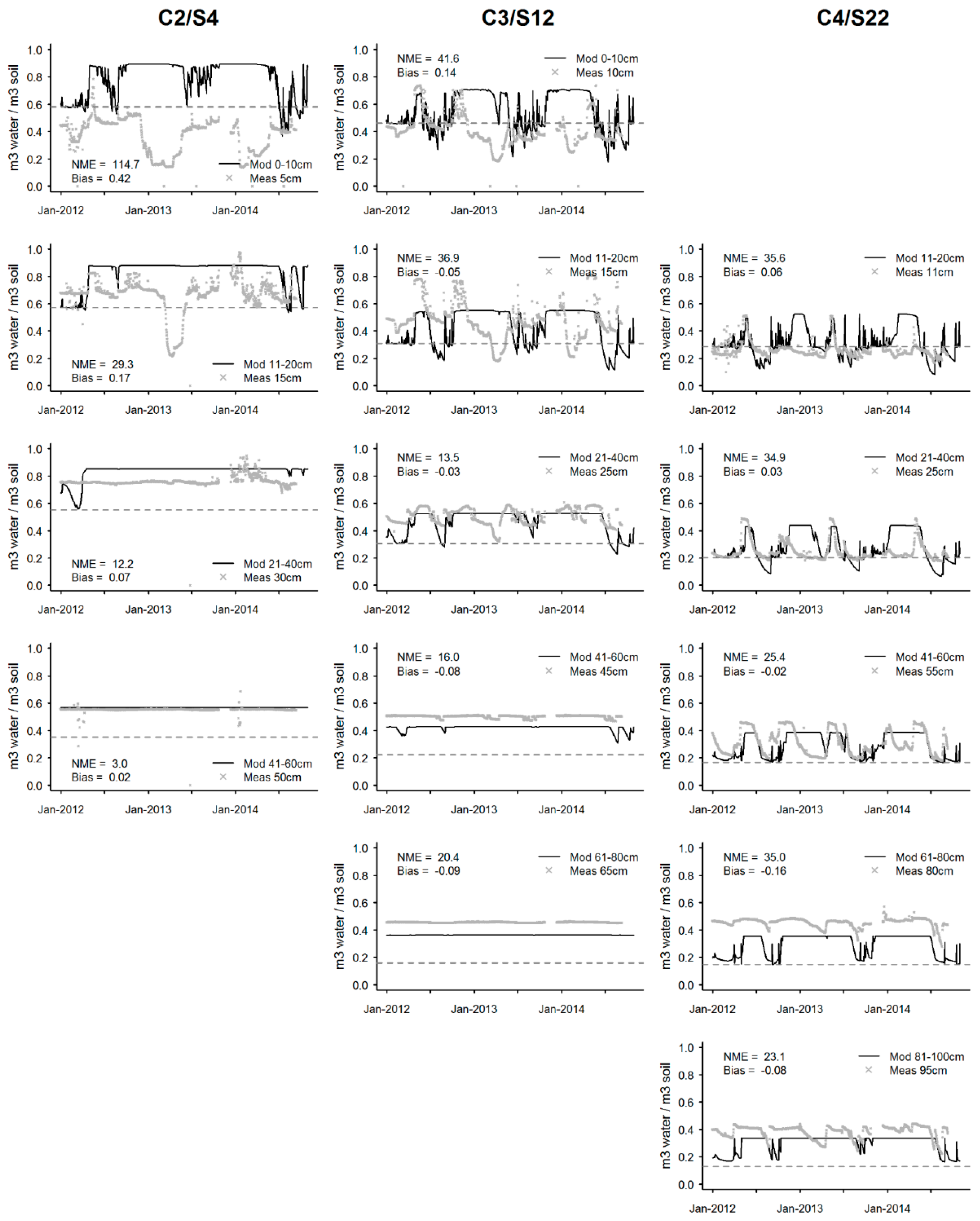
4.2. Soil Moisture
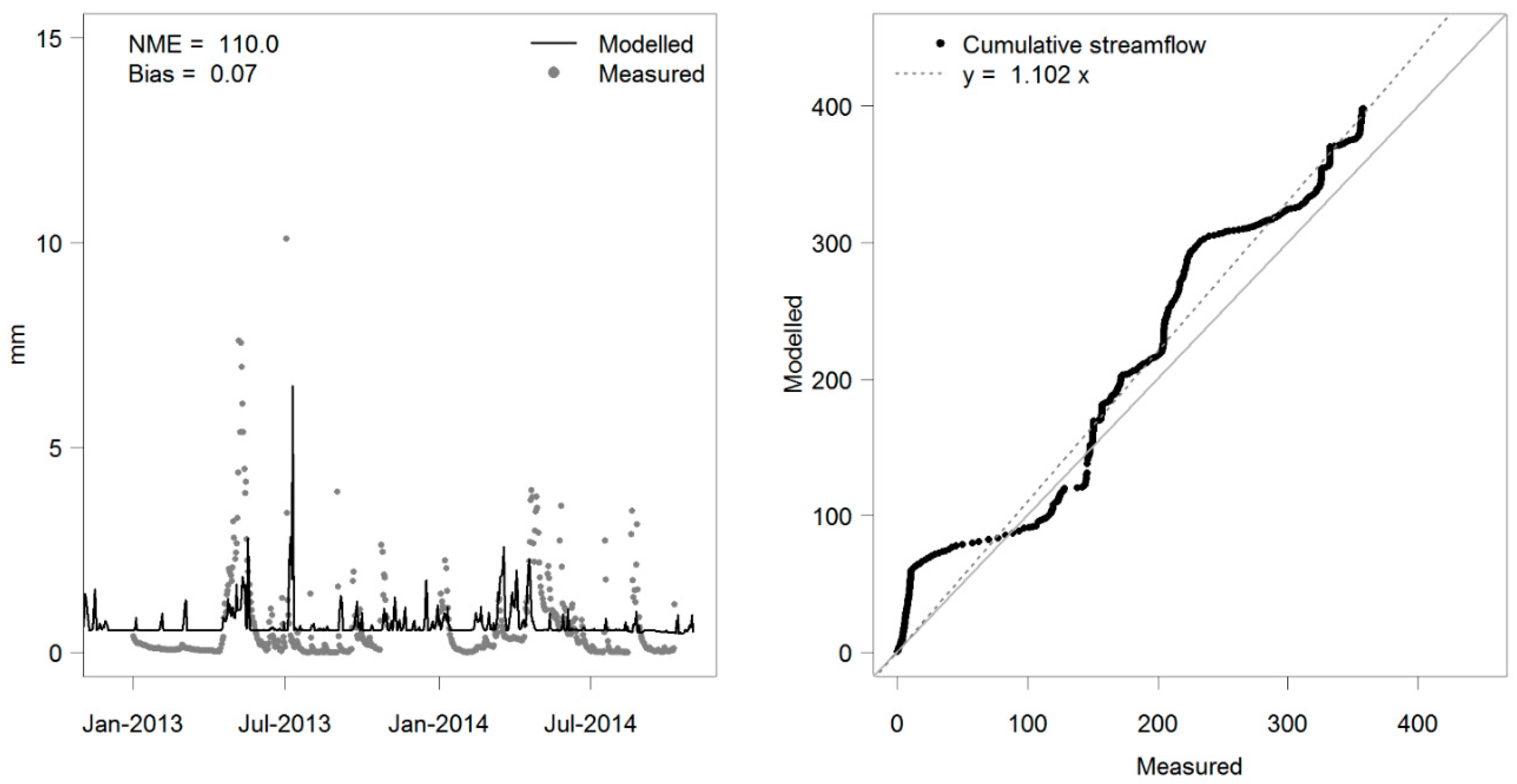
4.3. Streamflow
5. Conclusions
Supplementary Material
Acknowledgments
Author Contributions
Conflicts of Interest
References and Notes
- Chang, M. Forest Hydrology: An Introduction to Water and Forests, 2nd ed.; CRC Press: Boca Raton, FL, USA, 2006. [Google Scholar]
- Neary, D.G.; Ice, G.G.; Jackson, C.R. Linkages between forest soils and water quality and quantity. For. Ecol. Manag. 2009, 258, 2269–2281. [Google Scholar] [CrossRef]
- FAO. Forest and Water-International Momentum and Action; FAO: Rome, Italy, 2013; p. 86. [Google Scholar]
- Muller, F.; Chang, K.-C.; Lee, C.-L.; Chapman, S. Effects of temperature, rainfall and conifer felling practices on the surface water chemistry of northern peatlands. Biogeochemistry 2015, 126, 343–362. [Google Scholar] [CrossRef]
- Hellsten, S.; Stadmark, J.; Pihl Karlsson, G.; Karlsson, P.E.; Akselsson, C. Increased concentrations of nitrate in forest soil water after windthrow in southern sweden. For. Ecol. Manag. 2015, 356, 234–242. [Google Scholar] [CrossRef]
- Taboada-Castro, M.M.; Rodríguez-Blanco, M.L.; Diéguez, A.; Palleiro, L.; Oropeza-Mota, J.L.; Taboada-Castro, M.T. Effects of changing land use from agriculture to forest on stream water quality in a small basin in nw spain. Commun. Soil Sci. Plant Anal. 2015, 46, 353–361. [Google Scholar] [CrossRef]
- Schelker, J.; Öhman, K.; Löfgren, S.; Laudon, H. Scaling of increased dissolved organic carbon inputs by forest clear-cutting—what arrives downstream? J. Hydrol. 2014, 508, 299–306. [Google Scholar] [CrossRef]
- Xiao, W.; Chun, Z.; Qing, J. Impacts of climate change on forest ecosystems in northeast china. Adv. Clim. Chang. Res. 2013, 4, 230–241. [Google Scholar] [CrossRef]
- Aber, J.; Neilson, R.P.; McNulty, S.; Lenihan, J.M.; Bachelet, D.; Drapek, R.J. Forest processes and global environmental change: Predicting the effects of individual and multiple stressors we review the effects of several rapidly changing environmental drivers on ecosystem function, discuss interactions among them, and summarize predicted changes in productivity, carbon storage, and water balance. Bioscience 2001, 51, 735–751. [Google Scholar]
- Campbell, J.L.; Rustad, L.E.; Boyer, E.W.; Christopher, S.F.; Driscoll, C.T.; Fernandez, I.J.; Groffman, P.M.; Houle, D.; Kiekbusch, J.; Magill, A.H.; et al. Consequences of climate change for biogeochemical cycling in forests of northeastern north americathis article is one of a selection of papers from ne forests 2100: A synthesis of climate change impacts on forests of the northeastern us and eastern canada. Can. J. For. Res. 2009, 39, 264–284. [Google Scholar] [CrossRef]
- Belyazid, S.; Westling, O.; Sverdrup, H. Modelling changes in forest soil chemistry at 16 Swedish coniferous forest sites following deposition reduction. Environ. Pollut. 2006, 144, 596–609. [Google Scholar] [CrossRef] [PubMed]
- Gaudio, N.; Belyazid, S.; Gendre, X.; Mansat, A.; Nicolas, M.; Rizzetto, S.; Sverdrup, H.; Probst, A. Combined effect of atmospheric nitrogen deposition and climate change on temperate forest soil biogeochemistry: A modeling approach. Ecol. Model. 2015, 306, 24–34. [Google Scholar] [CrossRef] [Green Version]
- Homann, P.S.; McKane, R.B.; Sollins, P. Belowground processes in forest-ecosystem biogeochemical simulation models. For. Ecol. Manag. 2000, 138, 3–18. [Google Scholar] [CrossRef]
- Maxwell, R.M.; Putti, M.; Meyerhoff, S.; Delfs, J.-O.; Ferguson, I.M.; Ivanov, V.; Kim, J.; Kolditz, O.; Kollet, S.J.; Kumar, M.; et al. Surface-subsurface model intercomparison: A first set of benchmark results to diagnose integrated hydrology and feedbacks. Water Resour. Res. 2014. [Google Scholar] [CrossRef]
- Wallman, P.; Svensson, M.G.E.; Sverdrup, H.; Belyazid, S. Forsafe—An integrated process-oriented forest model for long-term sustainability assessments. For. Ecol. Manag. 2005, 207, 19–36. [Google Scholar] [CrossRef]
- Yu, L.; Belyazid, S.; Akselsson, C.; van der Heijden, G.; Zanchi, G. Storm disturbances in a swedish forest—A case study comparing monitoring and modelling. Ecol. Model. 2016, 320, 102–113. [Google Scholar] [CrossRef]
- Zanchi, G.; Belyazid, S.; Akselsson, C.; Yu, L. Modelling the effects of management intensification on multiple forest services: A swedish case study. Ecol. Model. 2014, 284, 48–59. [Google Scholar] [CrossRef]
- Richmond, B. An Introduction to System Thinking with Stella; Isee Systems Inc: Lebanon, NH, USA, 2004. [Google Scholar]
- Lindström, G.; Gardelin, M. Chapter 3.1: Hydrological Modelling-Model Structure. In Modelling Groundwater Response to Acidification; Swedish Meteorological and Hydrological Institute (SMHI): Norrköping, Sweden, 1992; pp. 33–36. [Google Scholar]
- Balland, V.; Pollacco, J.A.P.; Arp, P.A. Modeling soil hydraulic properties for a wide range of soil conditions. Ecol. Model. 2008, 219, 300–316. [Google Scholar] [CrossRef]
- Saxton, K.E.; Rawls, W.J. Soil water characteristic estimates by texture and organic matter for hydrologic solutions. Soil Sci. Soc. Am. J. 2006, 70, 1569–1578. [Google Scholar] [CrossRef]
- Reid, I. The choice of assumed particle density in soil tests. Area 1973, 5, 10–12. [Google Scholar]
- Bergström, S. The HBV Model: Its Structure and Applications; Swedish Meteorological and Hydrological Institute (SMHI): Nörrköping, Sweden, 1992; p. 35. [Google Scholar]
- Dingman, S.L. Physical hydrology, 2nd ed.; Waveland Press, Inc.: Long Grove, IL, USA, 2008; p. 646. [Google Scholar]
- Rosengren, U.; Stjernquist, I. Gå på djupet!: Om rotdjup och rotproduktion i olika skogstyper; SUFOR: Alnarp, Sweden, 2004; p. 55. [Google Scholar]
- Laudon, H.; Taberman, I.; Ågren, A.; Futter, M.; Ottosson-Löfvenius, M.; Bishop, K. The krycklan catchment study—a flagship infrastructure for hydrology, biogeochemistry, and climate research in the boreal landscape. Water Resour. Res. 2013, 49, 7154–7158. [Google Scholar] [CrossRef]
- Nyberg, L.; Stähli, M.; Mellander, P.-E.; Bishop, K.H. Soil frost effects on soil water and runoff dynamics along a boreal forest transect: 1. Field investigations. Hydrol. Process. 2001, 15, 909–926. [Google Scholar] [CrossRef]
- Lindqvist, G.; Nilsson, L.; Gonzalez, G. Depth of Till Overburden and Bedrock Fractures on the Svartberget Catchment as Determined by Different Geophisical Methods; University of Luleå: Luleå, Sweden, 1989; p. 16. [Google Scholar]
- Erlandsson, M.; Uppsala University, Uppsala, Sweden. Personal communication, 2015.
- Bishop, K.H. Episodic Increases in Stream Acidity, Catchment Flow Pathways and Hydrograph Separation; University of Cambridge: Cambridge, UK, 1991. [Google Scholar]
- Yi, S.; Manies, K.; Harden, J.; McGuire, A.D. Characteristics of organic soil in black spruce forests: Implications for the application of land surface and ecosystem models in cold regions. Geophys. Res. Lett. 2009. [Google Scholar] [CrossRef]
- Mitsch, W.J.; Gosselink, J.G. Wetlands, 5th ed.; Wiley: Hoboken, NJ, USA, 2015. [Google Scholar]
- Kellner, E. Wetland—Different Types, Their Properties and Functions; Department of Earth Sciences/Hydrology: Uppsala, Sweden, 2003; p. 62. [Google Scholar]
- Bishop, K.; Seibert, J.; Nyberg, L.; Rodhe, A. Water storage in a till catchment. Ii: Implications of transmissivity feedback for flow paths and turnover times. Hydrol. Process. 2011, 25, 3950–3959. [Google Scholar] [CrossRef]
- Rodhe, A. On the generation of stream runoff in till soils. Nord. Hydrol. 1988, 20, 1–8. [Google Scholar]
- Cuo, L.; Giambelluca, T.W.; Ziegler, A.D. Lumped parameter sensitivity analysis of a distributed hydrological model within tropical and temperate catchments. Hydrol. Process. 2011, 25, 2405–2421. [Google Scholar] [CrossRef]
- Amvrosiadi, N.; Bishop, K.; Grabs, T.; Beven, K.; Seibert, J. Water storage dynamics in a till hillslope: The foundation for modeling flows and residence times. Hydrol. Process. 2015, submitted. [Google Scholar]
- Grip, H.; Rodhe, A. Vattnets väg från regn till back; Hallgren & Fallgren: Uppsala, Sweden, 2000. [Google Scholar]
- Bengtsson, L. Snowmelt estimated from energy budget studies. Nord. Hydrol. 1976, 7, 3–18. [Google Scholar]
- Grip, H.; Halldin, S.; Lindroth, A. Water use by intensively cultivated willow using estimated stomatal parameter values. Hydrol. Process. 1989, 3, 51–63. [Google Scholar] [CrossRef]


| Parameter | Description | Unit | Baseline | Range of Variation |
|---|---|---|---|---|
| WD | Transect length given by the distance from the river to the water divide | m | 110 | 80–140 |
| Kbott | Saturated hydraulic conductivity at the bottom of the soil column j, i.e., in layer (j,7) | m·d−1 | Ksat(j,7) × 0.5 | 0–Ksat(j,7) |
| FrStream | Fraction of bottom percolation reaching the stream | fraction | Linearly decreasing | 0.8–1.0 |
| Cmelt | Degree-day factor for snow melt | mm·°C−1 ·d−1 | 1.5 | 1–2 |
| LP | Limit for potential evapotranspiration, expressed as a fraction of FC | fraction | 0.65 × FC(j,i) | 0.5–0.8 × FC(j,i) |
| POR | Porosity of all soil layers | fraction | POR(j,i) | POR(j,i) ± 10% |
| Ksat | Saturated conductivity of all soil layers | m∙d−1 | Ksat(j,i) | Ksat(j,i) ± 10% |
| Scenario | Range | Snow | Saturated Storage | Unsaturated Storage | Streamflow, Q | Q 90% perc (Q90) | Q 10% perc (Q10) | ||||||
|---|---|---|---|---|---|---|---|---|---|---|---|---|---|
| Bias | RMSE | Bias | RMSE | Bias | RMSE | Bias | RMSE | Bias | RMSE | Bias | RMSE | ||
| WD | 140 m | 0.00 | 0.00 | 0.00 | 0.40 | −0.53 | 1.08 | −0.01 | 0.14 | 0.00 | 0.00 | 0.00 | 0.00 |
| 80 m | 0.00 | 0.00 | 0.01 | 0.76 | 0.78 | 1.71 | 0.02 | 0.21 | 0.02 | 0.02 | 0.01 | 0.01 | |
| Kbott | Ksat(j,7) | 0.00 | 0.00 | −0.31 | 4.05 | −6.02 | 7.59 | 0.00 | 0.41 | −0.02 | 0.02 | −0.01 | 0.01 |
| 0 | 0.00 | 0.00 | 348.27 | 399.01 | −186.35 | 223.42 | −0.15 | 1.34 | 0.34 | 0.34 | −0.09 | 0.09 | |
| FrStream | 1 | 0.00 | 0.00 | 0.00 | 0.00 | 0.00 | 0.00 | 0.06 | 0.14 | 0.10 | 0.10 | 0.00 | 0.00 |
| 0.8 | 0.00 | 0.00 | 0.00 | 0.00 | 0.00 | 0.00 | −0.08 | 0.17 | −0.14 | 0.14 | −0.01 | 0.01 | |
| Cmelt | 1 mm | 0.00 | 0.00 | 0.00 | 0.00 | 0.00 | 0.00 | 0.00 | 0.03 | 0.01 | 0.01 | 0.00 | 0.00 |
| 2 mm | −2.89 | 7.39 | −0.07 | 6.97 | −0.22 | 9.32 | 0.01 | 0.92 | 0.04 | 0.04 | −0.01 | 0.01 | |
| LP | 0.5 × FC | 0.00 | 0.00 | 0.00 | 0.15 | −2.48 | 3.79 | −0.02 | 0.06 | −0.01 | 0.01 | 0.00 | 0.00 |
| 0.8 × FC | 0.00 | 0.00 | 0.00 | 0.63 | 3.56 | 5.28 | 0.02 | 0.11 | 0.05 | 0.05 | 0.00 | 0.00 | |
| POR | −10% | 0.00 | 0.00 | 0.17 | 3.19 | −34.49 | 34.83 | 0.01 | 0.38 | 0.00 | 0.00 | 0.00 | 0.00 |
| 10% | 0.00 | 0.00 | −0.10 | 2.29 | 34.49 | 34.71 | −0.02 | 0.22 | 0.04 | 0.04 | 0.00 | 0.00 | |
| Ksat | −10% | 0.00 | 0.00 | 0.03 | 0.54 | 2.37 | 2.63 | 0.00 | 0.10 | 0.02 | 0.02 | 0.00 | 0.00 |
| 10% | 0.00 | 0.00 | 0.00 | 1.29 | −2.04 | 2.55 | 0.00 | 0.12 | 0.02 | 0.02 | 0.00 | 0.00 | |
| Bias | RMSE | NME (%) | ||
|---|---|---|---|---|
| Soil moisture | C2:L2 | −0.101 | 0.242 | 34.8 |
| C2:L4 | −0.194 | 0.196 | 35.2 | |
| C3:L2 | −0.163 | 0.239 | 46.6 | |
| C3:L4 | −0.268 | 0.270 | 53.3 | |
| C4:L2 | 0.007 | 0.083 | 26.9 | |
| C4:L4 | −0.139 | 0.163 | 44.0 | |
| Streamflow | Q | −0.022 | 1.387 | 108.6 |
| Q90 | −0.664 | 0.664 | 37.4 | |
| Q10 | 0.103 | 0.103 | 683.1 |
| Year | T | Deep Perc | Stream Flow | R | ΔS | T + R + ΔS | P |
|---|---|---|---|---|---|---|---|
| 2011 | 368 | 3 | 52 | 55 | 225 | 648 | 649 |
| 2012 | 451 | 14 | 255 | 270 | 108 | 829 | 829 |
| 2013 | 441 | 15 | 250 | 265 | −64 | 641 | 642 |
| 2014 | 412 | 12 | 203 | 215 | −89 | 538 | 537 |
| Total | 1570 | 105 | 863 | 968 | 119 | 2657 | 2657 |
| % of P | 59% | 4% | 32% | 36% | 4% | 100% |
© 2016 by the authors; licensee MDPI, Basel, Switzerland. This article is an open access article distributed under the terms and conditions of the Creative Commons by Attribution (CC-BY) license (http://creativecommons.org/licenses/by/4.0/).
Share and Cite
Zanchi, G.; Belyazid, S.; Akselsson, C.; Yu, L.; Bishop, K.; Köhler, S.J.; Grip, H. A Hydrological Concept including Lateral Water Flow Compatible with the Biogeochemical Model ForSAFE. Hydrology 2016, 3, 11. https://doi.org/10.3390/hydrology3010011
Zanchi G, Belyazid S, Akselsson C, Yu L, Bishop K, Köhler SJ, Grip H. A Hydrological Concept including Lateral Water Flow Compatible with the Biogeochemical Model ForSAFE. Hydrology. 2016; 3(1):11. https://doi.org/10.3390/hydrology3010011
Chicago/Turabian StyleZanchi, Giuliana, Salim Belyazid, Cecilia Akselsson, Lin Yu, Kevin Bishop, Stephan J. Köhler, and Harald Grip. 2016. "A Hydrological Concept including Lateral Water Flow Compatible with the Biogeochemical Model ForSAFE" Hydrology 3, no. 1: 11. https://doi.org/10.3390/hydrology3010011