Regional Flood Frequency Analysis in the Volta River Basin, West Africa

Abstract

In the Volta River Basin, flooding has been one of the most damaging natural hazards during the last few decades. Therefore, flood frequency estimates are important for disaster risk management. This study aims at improving knowledge of flood frequencies in the Volta River Basin using regional frequency analysis based on L-moments. Hence, three homogeneous groups have been identified based on cluster analysis and a homogeneity test. By using L-moment diagrams and goodness of fit tests, the generalized extreme value and the generalized Pareto distributions are found suitable to yield accurate flood quantiles in the Volta River Basin. Finally, regression models of the mean annual flood with the size of the drainage area, mean basin slope and mean annual rainfall are proposed to enable flood frequency estimation of ungauged sites within the study area.

1. Introduction

Flood fatalities in Africa have increased dramatically over the past half-century [1]. In order to mitigate flood risk, efficient flood management is urgently needed. Flood management, and especially flood risk assessment, requires the estimation of the relation between flood magnitude and its probability of exceedance. The estimation of design floods for a site has been a common problem in some regions, and there is always great interest in this estimation process, particularly for ungauged basins or for sites characterized by a short sample length. For instance, the prediction of floods in ungauged or poorly-gauged basins is one of the main tasks of the PUB (Prediction in Ungauged Basins) initiative, which was launched from 2003–2012 by the International Association of Hydrological Sciences to engage the scientific community towards achieving major advances in the capacity to make reliable predictions in ungauged basins [2]. Two main methods are often used to solve the problem of the data scarcity. The first one is called regional flood frequency analysis (RFFA), which consist of using the spatial coherence of hydrological variables to provide regional estimates of flood quantiles, which are superior to at-site estimates even in the presence of moderate heterogeneity [3]. The second approach is the use of paleo flood data to extend the dataset in time. Although the use of paleo flood data if available increases the length of the time series for a more accurate estimation of flood quantiles, paleo flood data may contain many errors and may represent other climate and land use conditions not comparable with the actual situations.

With regard to RFFA in Africa, few studies were carried out. For instance, a regional flood frequency analysis based on L-moments is performed in the KwaZulu-Natal province of South Africa [4]. Kachroo et al. [5] and Mkhandi et al. [6] proposed some methodologies to delineate homogeneous regions and identify regional distributions for RFFA in Southern Africa. Padi et al. [7] performed a large-scale analysis of flood data in Africa using probabilistic regional envelope curves (PRECs). However, it was the first time an index-flood method with L-moments together was applied in West Africa, particularly in the Volta River Basin (VRB), in order to identify the suitable flood frequency distributions.

Several approaches, such as the index flood method, the regional shape estimation procedure, the “region of influence approach”, the hierarchical regions method, the fractional membership procedure, the Bayesian approach, PRECs and canonical correlation analysis, have been proposed for the purpose of RFFA. First, the index flood method was suggested by Dalrymple [8]. It assumes that sites within the same group are characterized by the same frequency distribution apart from a scaling factor called the index flood. In addition, the index flood method is based on the identification of homogeneous groups in which a relationship between the dimensionless flood and the return period is estimated. The homogeneous group is formed by basins, which are assumed to have similarities in meteorological and/or morphological characteristics. Secondly, the regional shape estimation method was proposed by Stedinger and Lu [9]. This method computes the location and scale parameters for each site, while the shape parameter is calculated by taking the average value in a group. Thirdly, the “region of influence” approach, developed by Burn [10], is based on the identification of a region of influence, which consists of sites with similar flood generation processes, and a weight must account for each site in the estimation of the quantiles. Another technique of regionalization is the hierarchical regions method [11], which defines first large regions wherein the coefficient of skewness is considered constant, and these regions are further divided into subgroups, wherein the coefficient of variation is supposed constant, as well. Then, a relationship is defined between the location parameter of the distribution and the climatic/physiographic characteristics. In the fractional membership method proposed by Wiltshire [12], the sites are assumed to have a fractional membership in many regions, rather than belonging to a particular region, and the parameters of the flood distribution can be estimated via a weighted average of the corresponding estimates for different regions. Bayesian methods have been applied to include regional information in flood frequency analysis [13,14,15]. In these methods, regional information is first used to define a prior distribution, which is further modified based on observed data at sites to provide a posterior distribution. PRECs were suggested by Castellarin [16] to estimate design floods at ungauged basins. In this approach, it is assumed that the flood frequency is homogeneous, and the flood quantiles are normalized by the drainage area (A) of the basin and then related to A by a double-logarithmic plot. Canonical correlation analysis (CCA) has been used for the purpose of regional flood frequency estimation [17,18]. CCA is a multivariate statistical method that permits establishing the interrelations that may exist between two groups of variables by identifying the linear combinations of the variables of the first group that are the most correlated to some linear combinations of the variables of the second group [18]. Table 1 summarizes the advantages and disadvantages of some procedures of RFFA.

In this study, a RFFA has been performed for the VRB, West Africa. This is important because accurate at-site frequency analysis for the majority of the sites in the VRB is actually a great challenge due to the lack of flow gauging stations on many rivers and the short length of the available daily discharge data. More specifically, the paper applied the index flood methods based on L-moments [19].

The main aim of this study is to determine appropriate flood frequency distributions that enable adequate estimation of design floods in the VRB. Particularly, three research questions relevant to the development of a flood frequency model are investigated: (i) what are the best probability distributions of describing annual maximum discharges (AMAX) in the VRB context? (ii) What are the best multi-regression models that could be used for estimating AMAX, particularly at ungauged sites in the study area? (iii) What are the characteristics of AMAX in the VRB?

Table 1. Pros and cons of some regional flood frequency estimation methods. RFFA, flood frequency analysis.

RFFA Methods	Advantages	Disadvantages
Index flood method	The multiplication of regional estimate with at-site statistic reduces the uncertainties associated with regionalization.	This method is sensitive to the homogeneity assumption and the formation of regions.
Regional shape estimation method	This method is more effective when higher-order L-moment ratios are equal at each site.	The conditions for good performance of this method are not physically plausible.
Region of influence method	The explicit construction of a region is not necessary.	It is difficult to define the appropriate weights.
Hierarchical approach	This method uses more information to estimate the distribution parameters.	This method may produce abrupt changes in the parameters from one site to another.
Fractional membership approach	The explicit construction of a region is not necessary.	It is difficult to define the appropriate weights.
Bayesian method	This model accounts for sources of uncertainty, and the homogeneity of the sites is not required.	The prior distributions of parameters are not precise and do not add more precision to the estimates [3].
Probability regional envelope curves	This method is more effective to estimate very high flood quantiles.	The logarithmic transformations may introduce biases in the estimates.
Canonical correlation analysis method	Possibility to predict multiple dependent variables from multiple independent variables.	One is constrained to identify linear relationship, which may not be reasonable.

Table 1. Pros and cons of some regional flood frequency estimation methods. RFFA, flood frequency analysis.

RFFA Methods	Advantages	Disadvantages
Index flood method	The multiplication of regional estimate with at-site statistic reduces the uncertainties associated with regionalization.	This method is sensitive to the homogeneity assumption and the formation of regions.
Regional shape estimation method	This method is more effective when higher-order L-moment ratios are equal at each site.	The conditions for good performance of this method are not physically plausible.
Region of influence method	The explicit construction of a region is not necessary.	It is difficult to define the appropriate weights.
Hierarchical approach	This method uses more information to estimate the distribution parameters.	This method may produce abrupt changes in the parameters from one site to another.
Fractional membership approach	The explicit construction of a region is not necessary.	It is difficult to define the appropriate weights.
Bayesian method	This model accounts for sources of uncertainty, and the homogeneity of the sites is not required.	The prior distributions of parameters are not precise and do not add more precision to the estimates [3].
Probability regional envelope curves	This method is more effective to estimate very high flood quantiles.	The logarithmic transformations may introduce biases in the estimates.
Canonical correlation analysis method	Possibility to predict multiple dependent variables from multiple independent variables.	One is constrained to identify linear relationship, which may not be reasonable.

2. Methodology

In this study, we apply the index flood method based on L-moments, as reported by Hosking and Wallis [19]. The methods used in the present study are articulated in five steps: (i) screening of the data; (ii) identification of homogeneous groups; (iii) selection of the regional flood frequency distributions; (iv) development of regional growth curves; and (v) development of prediction equations for the mean annual flood.

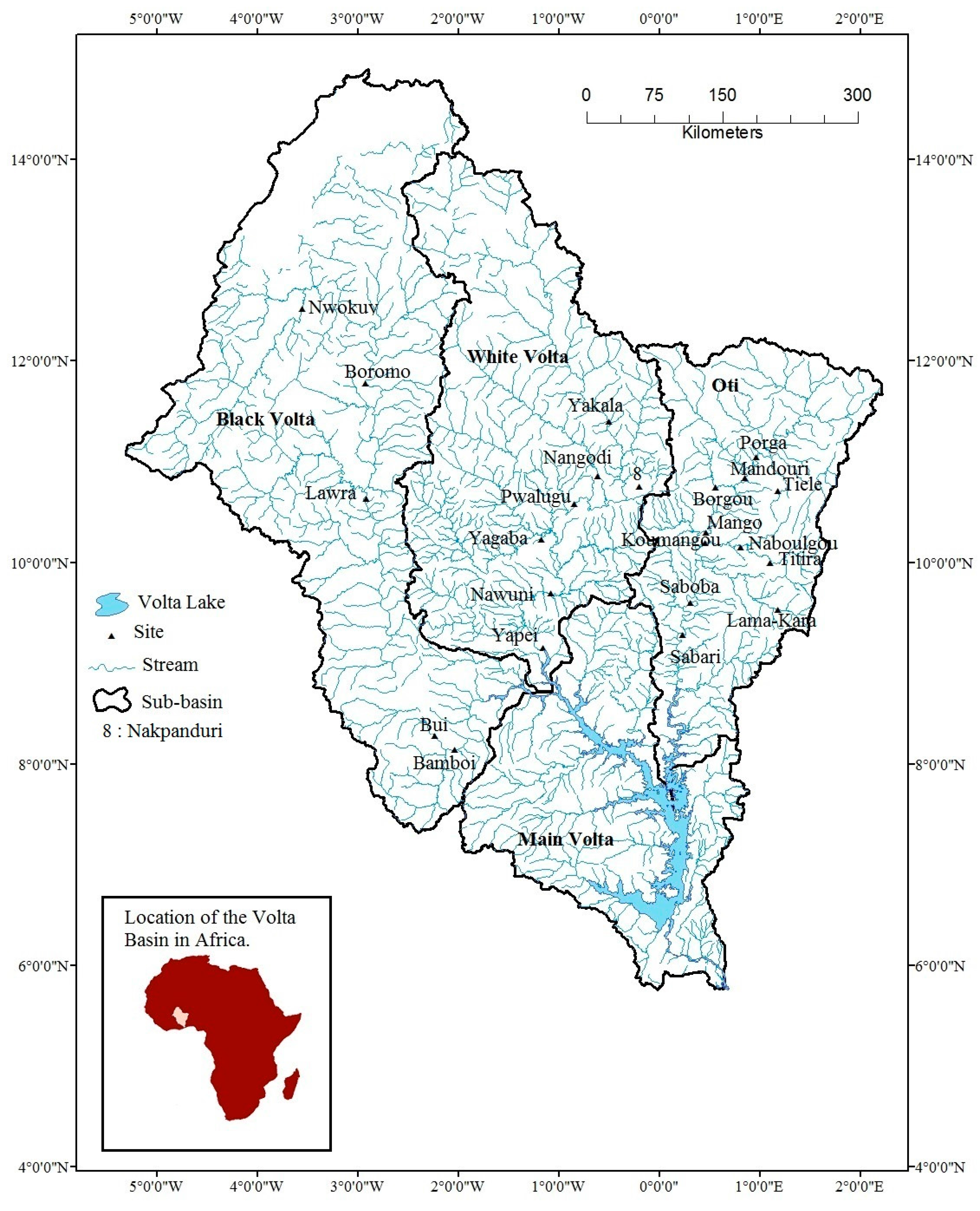
2.1. Study Area and Data

The present study is carried out in the Volta River Basin (VRB) of West Africa. Its geographic coordinates range from 5°30’W–2°00’E longitude–5°30’N–14°30’N latitude. The VRB covers a total area of about 400,000 km², and it is drained by four main rivers, namely the Black Volta, White Volta, Oti and Main Volta rivers (Figure 1). According to Amisigo [20], the mean annual discharge of the Black Volta River near its source is around 0.4 km³; the mean annual discharge of the White Volta River is about 0.2 km³ downstream of its source; and the Oti River joins the Main Volta with a flow of about 12.7 km³/year. In addition, the actual study sites are located upstream of the large Volta Lake created by the Akosombo Dam in Ghana. Twenty three flow gauging stations were selected for this study and the main criteria used to choose the sites were based on the length of record periods (minimum of thirteen years) and continuity (no consecutive gaps). Specifically, the AMAX were obtained for the years 1950–1973 for the White Volta and Black Volta from Moniod et al. [21] and for the years 1959–1990 for the Oti River. The mean annual precipitation values (1956–1974) for the sites of the White and Black Volta sub-basins were obtained from Moniod et al. [21], while some mean annual precipitation values (1975–2007) for the Oti River sub-basin were computed based on observed daily rainfall data. Table 2 and Table 3 show respectively the inter-site correlation of the AMAX and characteristics of the sub-basins (sites) used in this study.

2.2. L-Moment

L-moments are improvements over ordinary product moments. They are used to characterize the shape of a frequency distribution and estimate the parameters of this distribution, especially for a small size of environmental data [19]. For a detail description of L-moments, the reader is referred to Hosking [22]. The sample L-moments can be estimated using Equation (1) [22]:

$$l_{r+1}={\displaystyle \sum }_{k=0}^r{P}_{r,k}^{*} b_k$$

(1)

$P_{r,k}^{*}$ and $b_r$ are given in Equations (2) and (3), respectively. $l_{r+1}$ is the (r + 1)-th L-moment of the sample.

$$P_{r,k}^{*}={\left(-1\right)}^{r-k}\left(\begin{array}{c}r\\ k\end{array}\right)\left(\begin{array}{c}r+k\\ k\end{array}\right)$$

(2)

$$b_r=n^{-1}{\displaystyle \sum }_{j=1}^n\frac{\left(j-1\right)\left(j-2\right)\dots .\left(j-r\right)}{\left(n-1\right)\left(n-2\right)\dots .\left(n-r\right)}{x}_j$$

(3)

where $x_j$, for j = 1,…,n, is the ordered sample and n is the sample size. Moreover, in RFFA based on L-moments, L-moments ratios of the sample are estimated using Equation (4):

$$t_r=\frac{l_r}{l_2}$$

(4)

where $t_r$ is the r-th sample L-moment ratio and $l_r$ is the r-th sample L-moment. Specifically, the sample L-coefficient of variation (L-cv) is t = $l_2/l_1$, while the sample L coefficient of skewness (L-skew) is $t_3=l_3/l_2$, and the sample L-coefficient of kurtosis (L-kur) is $t_4=l_4/l_2$ [22].

Figure 1. Location of the study area and the flow gauge stations.

Figure 1. Location of the study area and the flow gauge stations.

Table 2. Inter-site correlation of annual maximum discharges (AMAX) in the Volta River Basin.

Stations	Periods	Inter-Site Correlation Squared (R2 )
Nwokuy, Boromo	1955–1973	0.19
Boromo, Lawra	1955–1973	0.06
Lawra, Bui	1954–1973	0.01
Bui, Bamboi	1954–1973	0.01
Yakala, Nangodi	1958–1973	0.10
Nangodi, Nakpanduri	1958–1972	0.37
Nakpanduri, Pwalugu	1958–1972	0.21
Pwalugu, Yagaba	1958–1973	0.00
Yagaba, Nawuni	1958–1973	0.00
Nawuni, Yapei	1953–1967	0.00
Tiele, Porga	1963–1973	0.21
Porga, Mandouri	1963–1979	0.00
Mandouri, Borgou	1960–1979	0.00
Borgou, Mango	1960–1987	0.00
Mandouri, Mango	1959–1979	0.01
Mango, Titira	1962–1987	0.11
Titira, Naboulgou	1962–1987	0.62
Naboulgou, Koumangou	1962–1987	0.00
Koumangou, Lama-Kara	1959–1987	0.03
Lama-Kara, Saboba	1959–1987	0.00
Mango, Saboba	1959–1989	0.00
Saboba, Sabari	1959–1990	0.71

Table 2. Inter-site correlation of annual maximum discharges (AMAX) in the Volta River Basin.

Stations	Periods	Inter-Site Correlation Squared (R2 )
Nwokuy, Boromo	1955–1973	0.19
Boromo, Lawra	1955–1973	0.06
Lawra, Bui	1954–1973	0.01
Bui, Bamboi	1954–1973	0.01
Yakala, Nangodi	1958–1973	0.10
Nangodi, Nakpanduri	1958–1972	0.37
Nakpanduri, Pwalugu	1958–1972	0.21
Pwalugu, Yagaba	1958–1973	0.00
Yagaba, Nawuni	1958–1973	0.00
Nawuni, Yapei	1953–1967	0.00
Tiele, Porga	1963–1973	0.21
Porga, Mandouri	1963–1979	0.00
Mandouri, Borgou	1960–1979	0.00
Borgou, Mango	1960–1987	0.00
Mandouri, Mango	1959–1979	0.01
Mango, Titira	1962–1987	0.11
Titira, Naboulgou	1962–1987	0.62
Naboulgou, Koumangou	1962–1987	0.00
Koumangou, Lama-Kara	1959–1987	0.03
Lama-Kara, Saboba	1959–1987	0.00
Mango, Saboba	1959–1989	0.00
Saboba, Sabari	1959–1990	0.71

Table 3. Site characteristics used in the RFFA. L-cv, L-coefficient of variation; L-kur, L-coefficient of kurtosis.

Number	Site Name	River	Area (km2)	Main Slope (%)	Sample Length (Year)	L-cv	L-skew	L-kur
1	Nwokuy	Black Volta	14,800	0.70	20	0.20	0.06	0.24
2	Boromo	Black Volta	35,000	0.40	19	0.15	0.01	0.06
3	Lawra	Black Volta	66,820	1.10	23	0.23	0.15	0.10
4	Bui	Black Volta	96,000	1.47	20	0.26	0.25	0.30
5	Bamboi	Black Volta	134,200	0.11	24	0.25	0.20	0.19
6	Yakala	White Volta	31,680	1.19	18	0.22	−0.03	−0.04
7	Nangodi	Red Volta	11,570	1.41	16	0.25	0.03	0.10
8	Nakpanduri	White Volta	1530	1.47	15	0.23	−0.05	0.04
9	Pwalugu	White Volta	63,350	1.09	16	0.22	0.00	0.07
10	Yagaba	White Volta	10,600	0.45	16	0.26	−0.23	0.11
11	Nawuni	White Volta	92,950	1.05	21	0.13	−0.31	0.20
12	Yapei	White Volta	102,170	1.11	17	0.19	0.04	0.09
13	Tiele	Magou	836	1.56	13	0.17	0.21	0.16
14	Porga	Pendjari	22,280	0.33	27	0.28	0.13	0.13
15	Mandouri	Oti	29,100	0.80	21	0.21	0.01	−0.03
16	Borgou	Sansargou	2280	0.99	28	0.31	−0.03	0.06
17	Mango	Oti	35,650	0.33	37	0.32	0.23	0.07
18	Titira	Keran	3695	0.89	26	0.31	0.06	−0.04
19	Naboulgou	Keran	5470	1.153	26	0.19	0.01	0.06
20	Koumangou	Koumangou	6730	0.70	29	0.14	−0.03	0.19
21	Lama-Kara	Kara	1560	2.52	34	0.26	0.06	0.06
22	Saboba	Oti	53,090	1.44	32	0.24	0.11	0.01
23	Sabari	Oti	58,670	0.49	32	0.28	0.10	0.01

Table 3. Site characteristics used in the RFFA. L-cv, L-coefficient of variation; L-kur, L-coefficient of kurtosis.

Number	Site Name	River	Area (km2)	Main Slope (%)	Sample Length (Year)	L-cv	L-skew	L-kur
1	Nwokuy	Black Volta	14,800	0.70	20	0.20	0.06	0.24
2	Boromo	Black Volta	35,000	0.40	19	0.15	0.01	0.06
3	Lawra	Black Volta	66,820	1.10	23	0.23	0.15	0.10
4	Bui	Black Volta	96,000	1.47	20	0.26	0.25	0.30
5	Bamboi	Black Volta	134,200	0.11	24	0.25	0.20	0.19
6	Yakala	White Volta	31,680	1.19	18	0.22	−0.03	−0.04
7	Nangodi	Red Volta	11,570	1.41	16	0.25	0.03	0.10
8	Nakpanduri	White Volta	1530	1.47	15	0.23	−0.05	0.04
9	Pwalugu	White Volta	63,350	1.09	16	0.22	0.00	0.07
10	Yagaba	White Volta	10,600	0.45	16	0.26	−0.23	0.11
11	Nawuni	White Volta	92,950	1.05	21	0.13	−0.31	0.20
12	Yapei	White Volta	102,170	1.11	17	0.19	0.04	0.09
13	Tiele	Magou	836	1.56	13	0.17	0.21	0.16
14	Porga	Pendjari	22,280	0.33	27	0.28	0.13	0.13
15	Mandouri	Oti	29,100	0.80	21	0.21	0.01	−0.03
16	Borgou	Sansargou	2280	0.99	28	0.31	−0.03	0.06
17	Mango	Oti	35,650	0.33	37	0.32	0.23	0.07
18	Titira	Keran	3695	0.89	26	0.31	0.06	−0.04
19	Naboulgou	Keran	5470	1.153	26	0.19	0.01	0.06
20	Koumangou	Koumangou	6730	0.70	29	0.14	−0.03	0.19
21	Lama-Kara	Kara	1560	2.52	34	0.26	0.06	0.06
22	Saboba	Oti	53,090	1.44	32	0.24	0.11	0.01
23	Sabari	Oti	58,670	0.49	32	0.28	0.10	0.01

2.3. Data Screening

In order to check for errors in the data, outliers and trends, the discordancy measure $\left(D_i\right)$ for a site i as shown in Equation (5) was applied to the AMAX series of the 23 gauge stations in the VRB. The critical value of $D_i$ depends on the number of sites (N). For N ≥ 15, D_i must be less than or equal to 3.0 for the site to be considered in the RFFA; otherwise, it is deleted from the dataset [19].

$$D_i=\frac{1 }{3}N{\left(U_i-\overline{U}\right)}^T{\left[\left(U_i-\overline{U}\right){\left(U_i-\overline{U}\right)}^T\right]}^{-1}\left(U_i-\overline{U}\right)$$

(5)

where U is the vector of L-moments and N is the number of sites. $\overline{U}$ is an average of $U.$

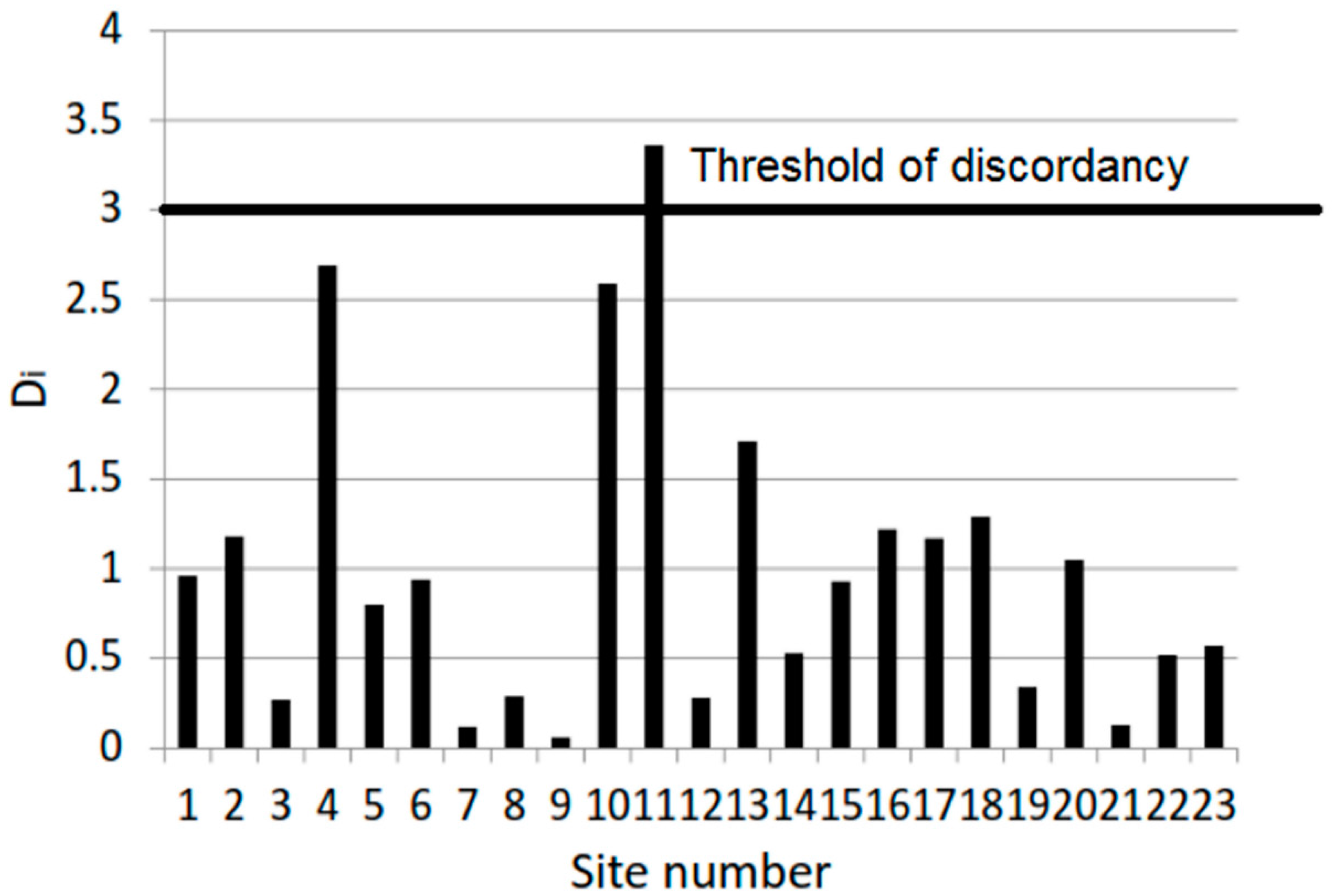
2.4. Identification of Homogeneous Groups

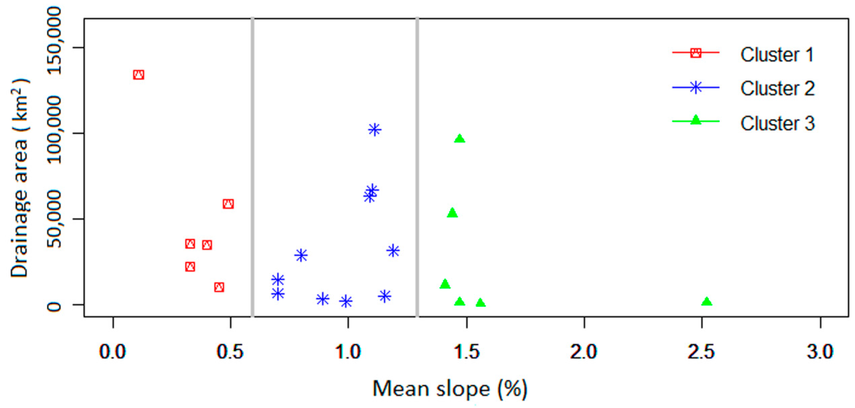
2.4.1. Cluster Analysis

The aim of the cluster analysis is to partition data into clusters in a way that sites belonging to the same cluster are similar regarding their climatic/physiographic characteristics. In this study, Ward’s algorithm [23] is used to form clusters with respect to the mean slope and drainage area of the basins, because this method is able to produce homogeneous clusters that have approximatively the same size.

Ward’s method is a hierarchical clustering that uses the increase in the total within-group sum of squares as a result of joining groups. The application of the hierarchical clustering was based on the standardized Euclidean distance (d), which is given by Equation (6) [24]:

$$d^2\left(p,q\right)=\left(x_p-x_q\right)D^{-1}{\left(x_p-x_q\right)}^T$$

(6)

where $x_p$ and $x_q$ are the coordinate of sites p and q in the physiographic space and $D^{-1}$ is a diagonal matrix. Since the variables are expressed in different units, each coordinate in the sum of squares is inverse weighted by the sample variance of that coordinate in order to eliminate the scale effects between the variables [24]. In addition, the within-group sum of squares (GSS) of a cluster is defined as the sum of the distance between all objects in the cluster and its center of gravity. It can be expressed by Equation (7) [24]:

$$GS{S}_r={\displaystyle \sum }_{i=1}^{n_r}{d}^2\left(x_{ri}-{\overline{x}}_r\right)$$

(7)

where $n_r$ and ${\overline{x}}_r$ are respectively the size and the centroid of cluster r.

According to Hosking and Wallis [19], the results from the cluster analysis need not, and usually should not, be final. Many types of subjective adjustment of groups may be useful to improve the homogeneity of the clusters. In this study, a few sites were moved from one cluster to another, and one site was deleted after the cluster analysis in order to improve the homogeneity of the groups.

2.4.2. Homogeneity Test

To identify the homogeneous groups, a homogeneity test was first applied to the Volta River Basin as a single region and secondly to the clusters. The principle of the homogeneity test is to compare the observed variations in L-moments ratios for the sites in each region with the ones that would be expected for a homogeneous region [19]. The variations in L-moments are computed as the standard deviation of at site L-cv weighted proportionally to the data length at each site. In order to ascertain what would be the variation in L-moments ratios for a homogeneous region, the four-parameter kappa distribution is fitted to the regional average L-moment ratios to generate a large number (greater than or equal to 500) of Monte Carlo simulations. The kappa distribution is chosen because it is a generalized distribution that produces many distributions as particular cases of the parameter values [19]. The heterogeneity measure, $H_j$ (j = 1, 2, 3) is given by Equation (8):

$$H_j=\frac{V_{j-}{\mu }_{v_j}}{{\sigma }_{v_j}}$$

(8)

where $H_1$ is the heterogeneity measure based on observed V₁, which is the weighted standard deviation of t values, $H_2$ is the heterogeneity measure based on observed V₂, which is the weighted standard deviation of (t/t₃) distance, $H_3$ is the heterogeneity measure based on observed V₃, which is the weighted standard deviation of (t₃/t₄) distance, and ${\mu }_{v_j}$ and ${\sigma }_{v_j}$ are the mean and standard deviation of the simulated values of V_j. According to Hosking and Wallis [19], a group is “acceptably homogeneous” if $H_j<$ 1, “possibly heterogeneous” if 1 $\le H_j$ $<$2 and “definitely heterogeneous” if $H_j\ge$ 2.

2.5. Selection of the Regional Flood Frequency Distribution

The next step after the formation of homogeneous groups is to choose the best distribution for each homogeneous group. The selection of the distribution that will yield the accurate quantiles was thus carried out in this work by first applying the L-moment diagram method to the homogeneous groups. L-moment diagrams are useful for evaluating which distribution(s), among a suite of possible models, provides a satisfactory approximation to the distribution of a particular hydrologic variable in a region [25]. In L-moment ratio diagrams, the sample L-skewness versus the sample L-kurtosis is plotted on a graph with the theoretical L-moment ratios of the candidate distributions. On these diagrams, a three-parameter distribution is plotted as a line, and the best distribution is the one whose line is closer to the majority of the sample data. Nevertheless, the graph may not have a good power of discrimination when many probability distributions are suitable for the sample data in L-moment ratio diagrams. For this reason, a numerical goodness of fit test, called the Z-statistic, is secondly applied to choose the best frequency distributions. This numerical test is based on the comparison between sample L-kurtosis and population L-kurtosis for the selected theoretical distributions. The test statistic, called $Z^{Dist}$, is defined in Equation (9) as follows:

$$Z^{Dist}=\left({\tau }_4^{Dist}-t_4^R+B_4\right)/{\sigma }_4$$

(9)

where $D_{ist}$ refers to a particular distribution, ${\tau }_4^{Dist}$ is the L-kurtosis of the selected distribution, $t_4^R$ is the regional weighted average of sample L-kurtosis and $B_4$ and ${\sigma }_4$ are respectively the bias of $t_4^R$ and the standard deviation of sample L-kurtosis. For each of the groups, a kappa distribution with its parameters estimated from the fitting of the distribution to the regional average L-moments ratios is used to simulate a large number of realizations for the same region. The frequency distribution that has the smallest absolute $Z^{Dist}$ is chosen as the best among other possible frequency distributions. At a confidence level of 90%, the critical value of absolute $Z^{Dist}$ is 1.64 [19]. Finally, quantile-quantile plots were used to compare the estimated quantiles and the observed flood values and to check the validity of the estimates provided by a fitted theoretical distribution. Five three-parameter theoretical distributions, namely the generalized logistic distribution (GLO), the generalized extreme value distribution (GEV), the generalized Pareto distribution (GPA), the generalized normal distribution (GNO) and the Pearson Type III distribution (PE3), were considered in this study.

2.6. Development of Regional Growth Curves

In an RFFA using the index flood approach, a relationship is established between a flood quantile of a given return period Q (T), and an index flood (taken as the mean AMAX series, $Q_m$) by introducing a regional growth curve, $q_R$. This relationship is shown in Equation (10):

$$Q\left(T\right)=q_R*Q_m$$

(10)

T is the return period. Moreover, $q_R$ depends only on the parameters of the frequency distribution and the return periods. For instance, $q_R$ for the GPA distribution is given in Equations (11) and (12), while Equations (13) and (14) show the expressions of $q_R$ for the GEV distribution.

$$q_R=\epsilon +\frac{\alpha }{k}\left[1-{\left(\frac{1}{T}\right)}^k\right] \mathrm{for} k\ne 0$$

(11)

$$q_R=\epsilon -\alpha log\left(\frac{1}{T}\right) \mathrm{for} k=0$$

(12)

$$q_R=\epsilon +\frac{\alpha }{k}\left\{1-{\left[-log\left(\frac{T-1}{T}\right)\right]}^k\right\} \mathrm{for} k\ne 0$$

(13)

$$q_R=\epsilon -\alpha \left\{log\left[-log\left(\frac{T-1}{T}\right)\right]\right\} \mathrm{for} k=0$$

(14)

where $\alpha ,\epsilon \text{and} k$ are, respectively, the scale, location and shape parameters of the distributions.

2.7. Development of Regression Models

In order to estimate the flood quantile for a given return period, the value of the index flood ($Q_m$) is needed. Because of the dearth of observed discharge data at the ungauged basins, $Q_m$ cannot be calculated. In this case, a regression model between $Q_m$ and physiographic or climatic basin descriptors, such as the drainage area, slope, altitude and mean annual precipitation (depending on data availability), is often used to estimate the index flood at ungauged sites, because the variation in flow discharges is related to the variations in physiographic and climatic characteristics of the basin. Usually, the study area is split into regions that are not necessarily homogeneous [26]. In this study, regression models were estimated separately for the White and Black Volta basins and the Oti River Basin.

Furthermore, a stepwise multi-regression with the forward selection method has been used to choose the best regression models. This method adds one independent variable at a time, which increases the coefficient of determination (R²) value of the regression. We started with the drainage area (A) of the basins in the equations. Then, other independent variables, such as mean slope (S), mean annual precipitation (P) and, elevation, are checked one at a time, and the most significant is added to the model at each stage. The procedure was terminated when all of the independent variables not in the equations have no significant effect on R².

3. Results and Discussion

Figure 2 gives the discordancy measures of the sites. It appears that only Site Number 11 is discordant with a Di value of 3.36, and it was consequently deleted from the dataset. In addition, treating first the whole VRB as a single region, the values of the different heterogeneity measures $H_1$, $H_2$ and $H_3$ obtained were respectively 4.11, 3.02 and 2.77. Therefore, the VRB is “definitely heterogeneous”, and homogeneous groups need to be formed.

Figure 2. Discordancy measure (Di) of the different gauge sites.

Figure 2. Discordancy measure (Di) of the different gauge sites.

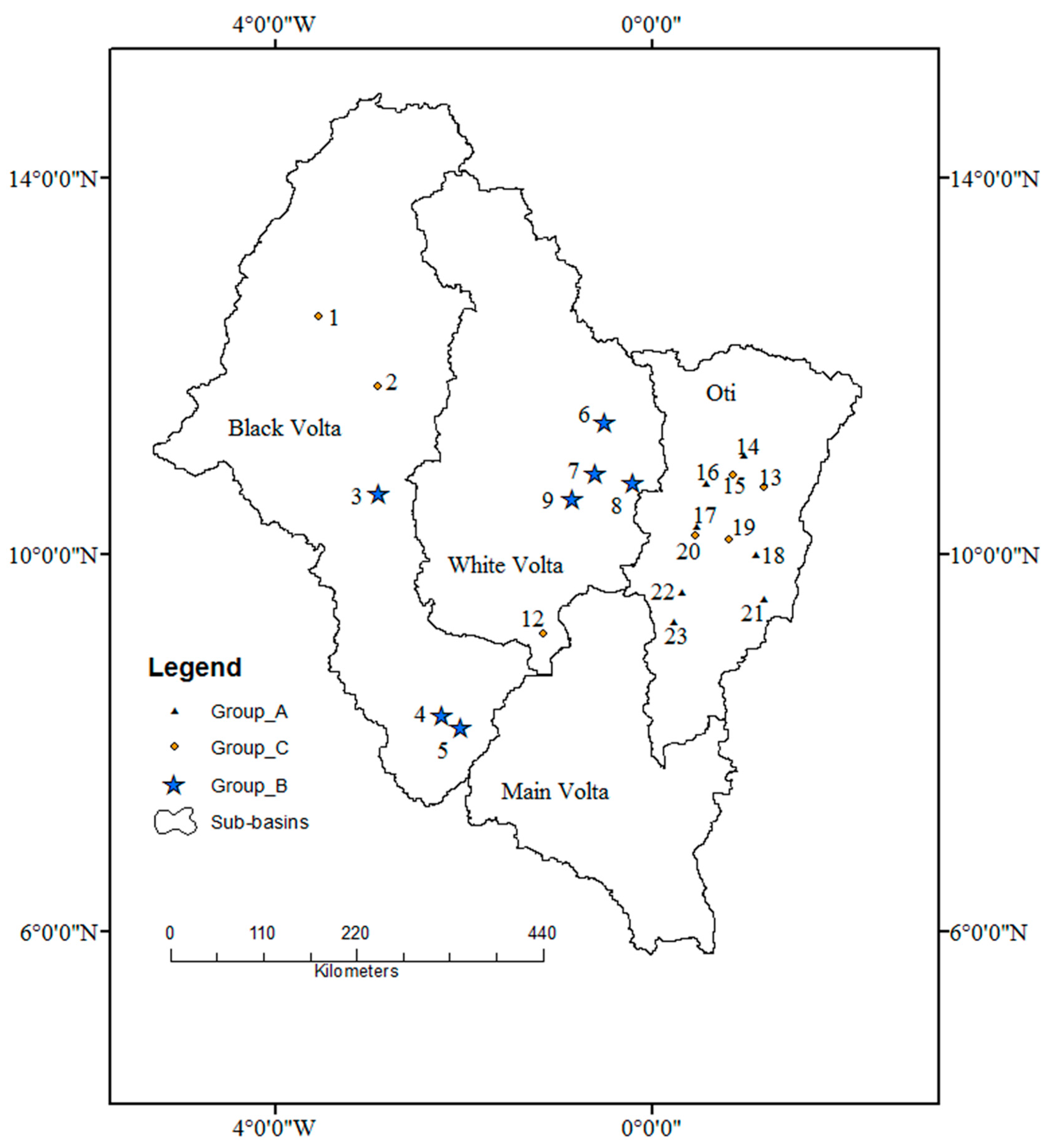
3.1. Formation of Homogeneous Groups

Figure 3 and Table 4 show the results of the cluster analysis. It can be seen from Table 4 that Cluster 1 is “acceptably homogeneous”, whereas Clusters 2 and 3 are “definitively heterogeneous”. Consequently, the clusters were adjusted to obtain the final groups shown in Table 5. It should be noted that the final groups are all “acceptably homogeneous”.

Figure 3. Formation of three groups through the cluster analysis.

Figure 3. Formation of three groups through the cluster analysis.

Table 4. Characteristics of the initial clusters.

Clusters	Number of Sites	H1	H2	H3	Homogeneity
1	6	0.44	−0.32	0.39	Homogeneous
2	10	4.48	3.19	2.69	Heterogeneous
3	6	1.65	2.30	3.03	Heterogeneous

Table 4. Characteristics of the initial clusters.

Clusters	Number of Sites	H1	H2	H3	Homogeneity
1	6	0.44	−0.32	0.39	Homogeneous
2	10	4.48	3.19	2.69	Heterogeneous
3	6	1.65	2.30	3.03	Heterogeneous

Table 5. Homogeneity measure of the final groups.

Groups	Number of Sites	H1	H2	H3	Homogeneity
A	7	0.12	0.29	0.43	Homogeneous
B	7	−2.02	0.70	0.98	Homogeneous
C	7	−0.21	−1.34	−0.37	Homogeneous

Table 5. Homogeneity measure of the final groups.

Groups	Number of Sites	H1	H2	H3	Homogeneity
A	7	0.12	0.29	0.43	Homogeneous
B	7	−2.02	0.70	0.98	Homogeneous
C	7	−0.21	−1.34	−0.37	Homogeneous

In addition, the location of the final homogeneous groups is shown in Figure 4. One can notice that all the sites of Group A are situated in the Oti River Basin, while those of Group B are located in the White and Black Volta basins. The sites of Group C are scattered in the White Volta, Black Volta and Oti basins. Similar results were found by Burn and Goel [27], who confirmed that in RFFA, the catchments of a given homogeneous region may not be geographically contiguous, but similar in terms of their flood generation processes.

Figure 4. Location of the final homogeneous groups (for the site characteristics; please see Table 3).

Figure 4. Location of the final homogeneous groups (for the site characteristics; please see Table 3).

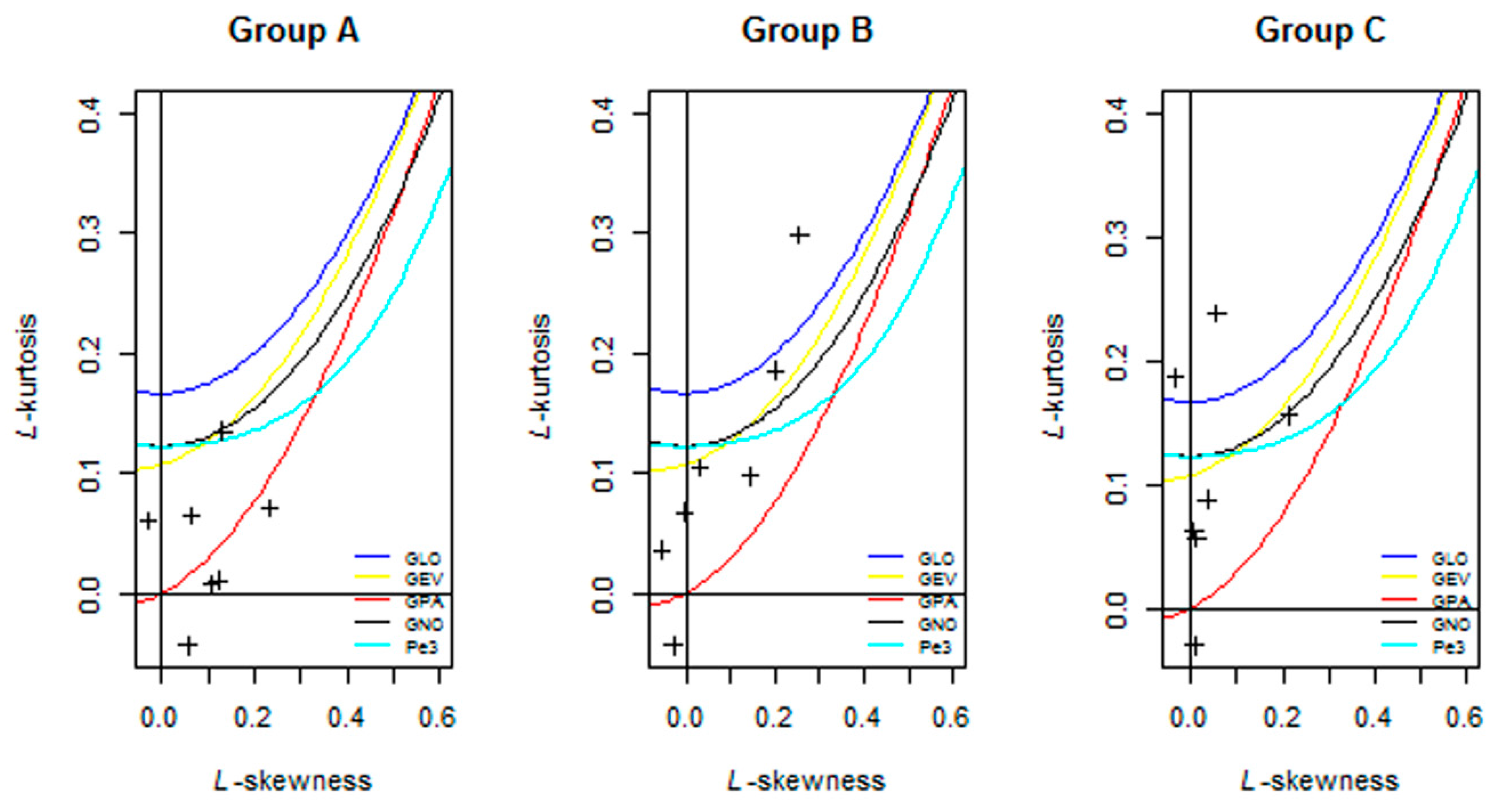
3.2. Selection of Appropriate Distributions

The choice of the appropriate distribution for each group is based on L-moment ratio diagrams, Z-statistic tests and quantile-quantile plots. First, Figure 5 shows the L-moment ratio diagrams for the homogeneous groups. It may be noted that the maximum of sample sites lies close to the GPA distribution line for Group A, whereas the sample sites are closer to the GEV and GPA distribution for both group B and Group C. Secondly, Table 6 summarizes the Z-statistic values of the appropriate candidate distributions for the homogeneous groups. In this table, it is observed that only the GPA distribution has the absolute value of the Z-statistic less than 1.64 for Group A and the GEV distribution has the lowest absolute value of the Z-statistic, which is less than 1.64, for both Group B and Group C. Hence, the GPA distribution can be considered as the regional distribution for Group A, while the GEV distribution is acceptable for both Groups B and C. These results are confirmed by the quantile-quantile plots for which the points lie approximately on the 1:1 line (Figure 6).

Table 6. Z-statistic values of the homogeneous groups.

Distribution	Group A	Group B	Group C
Generalized Pareto distribution	0.55	−2.57	−3.57
Generalized extreme value distribution	4.29	0.39	0.15
Pearson Type III distribution	4.20	0.40	0.55
Generalized normal distribution	4.45	0.52	0.56
Generalized logistic distribution	6.67	1.87	2.04

Table 6. Z-statistic values of the homogeneous groups.

Distribution	Group A	Group B	Group C
Generalized Pareto distribution	0.55	−2.57	−3.57
Generalized extreme value distribution	4.29	0.39	0.15
Pearson Type III distribution	4.20	0.40	0.55
Generalized normal distribution	4.45	0.52	0.56
Generalized logistic distribution	6.67	1.87	2.04

Figure 5. L-moment ratio diagrams for the homogeneous groups. GLO: generalized logistic distribution; GEV: generalized extreme value distribution; GPA: generalized Pareto distribution; GNO: generalized normal distribution; PE3: Pearson Type III distribution.

Figure 5. L-moment ratio diagrams for the homogeneous groups. GLO: generalized logistic distribution; GEV: generalized extreme value distribution; GPA: generalized Pareto distribution; GNO: generalized normal distribution; PE3: Pearson Type III distribution.

Figure 6. Quantile-quantile plots of the fitted frequency distributions for the three groups. GPA: generalized Pareto distribution; GEV: generalized extreme value distribution.

Figure 6. Quantile-quantile plots of the fitted frequency distributions for the three groups. GPA: generalized Pareto distribution; GEV: generalized extreme value distribution.

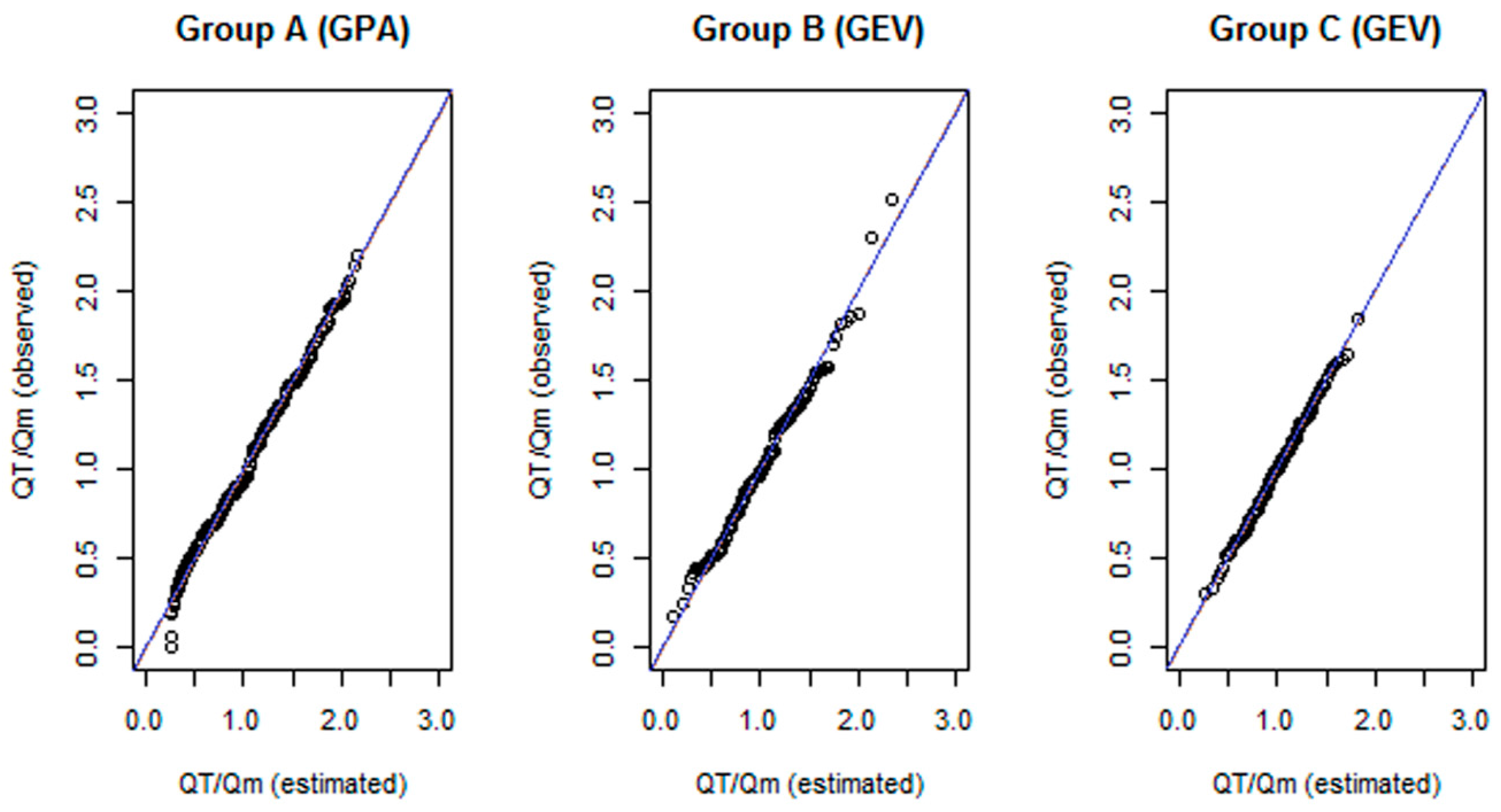
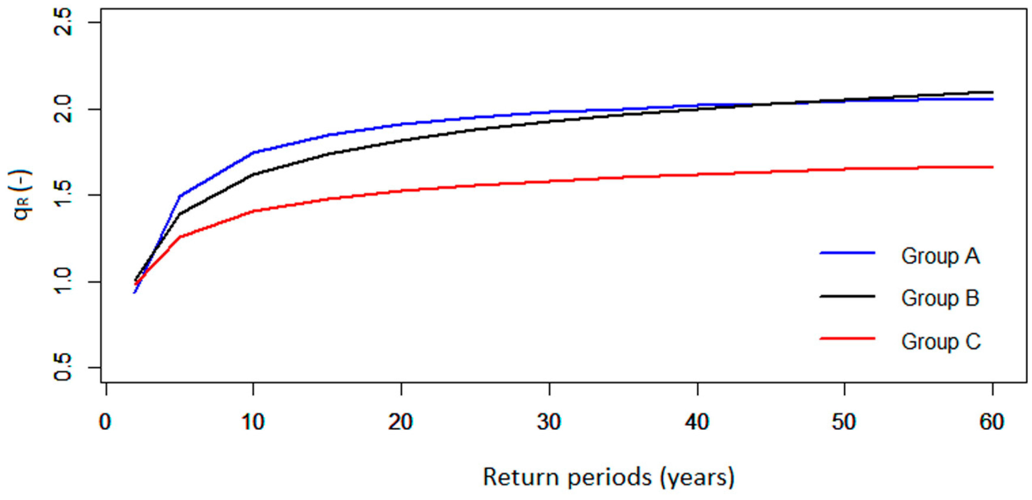
3.3. Flood Frequency Relationships

3.3.1. Regional Growth Curves

Table 7 and Figure 7 show respectively the quantile functions and the regional growth curves of the homogeneous groups. Table 7 shows also the fitted parameters to the distributions selected. In order to estimate the flood quantile for a given return period, Equation (10) is used. For the ungauged sites where observed discharge data are not available to compute the index flood ($Q_m)$, the values of $Q_m$ are estimated via a multi-regression model.

Table 7. Quantile functions of the homogeneous groups.

Group	Distributions and Their Parameters	Quantile Functions
A	GPA : ε = 0.25; α = 1.22; k = 0.62	$q_R$ = 0.25 + 1.97$\left\{1-{\left(\frac{1}{T}\right)}^{0.62}\right\}$
B style="border-bottom:solid thin"	GEV :ε = 0.82; α = 0.38; k = 0.12;	$q_R$ = 0.82 + 3.17$\left\{1-{\left[-ln\left(\frac{T-1}{T}\right)\right]}^{0.12}\right\}$
C	GEV: ε = 0.88; α = 0.30; k = 0.23	$q_R$ = 0.88 + 1.30$\left\{1-{\left[-ln\left(\frac{T-1}{T}\right)\right]}^{0.23}\right\}$

Table 7. Quantile functions of the homogeneous groups.

Group	Distributions and Their Parameters	Quantile Functions
A	GPA : ε = 0.25; α = 1.22; k = 0.62	$q_R$ = 0.25 + 1.97$\left\{1-{\left(\frac{1}{T}\right)}^{0.62}\right\}$
B style="border-bottom:solid thin"	GEV :ε = 0.82; α = 0.38; k = 0.12;	$q_R$ = 0.82 + 3.17$\left\{1-{\left[-ln\left(\frac{T-1}{T}\right)\right]}^{0.12}\right\}$
C	GEV: ε = 0.88; α = 0.30; k = 0.23	$q_R$ = 0.88 + 1.30$\left\{1-{\left[-ln\left(\frac{T-1}{T}\right)\right]}^{0.23}\right\}$

Figure 7. Regional growth curves of the homogeneous groups. $q_R=Q\left(T\right)/Q_m$; with $Q_m$, the index flood, and $Q\left(T\right)$, the flood quantile of return period T.

Figure 7. Regional growth curves of the homogeneous groups. $q_R=Q\left(T\right)/Q_m$; with $Q_m$, the index flood, and $Q\left(T\right)$, the flood quantile of return period T.

It can be seen from Figure 7 that the regional flood frequency curves for the different groups in the Volta Basin are relatively flat. This result confirms the findings of Meigh et al. [28], who showed that regional curves in West Africa and some regions affected by monsoon are “fairly flat”. Moreover, Sutcliffe and Farquharson [29], cited in Meigh et al. [28], noted that a feature of many basins with flat curves is that floods appear to be due to the accumulation of rainfall over a distinct wet season or monsoon and that the date of the annual maximum flood is relatively constant from year to year. This means that the peak flow is more likely to be related to the annual total rainfall, which is less variable than storm rainfall [28].

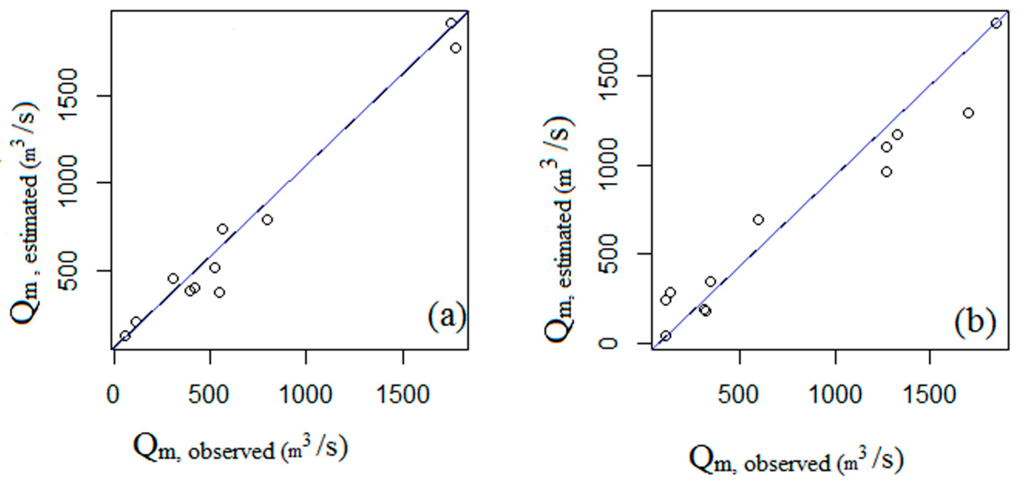
3.3.2. Regression Models

Table 8 and Figure 8 show respectively the best regression models and the comparison between estimated quantiles and the observed values of $Q_m$ (index flood). In these equations, A, P and S are respectively the drainage area, the mean annual precipitation and the mean slope of the basins. The powers associated with the area (0.61 and 0.8) are comparable to the findings of other similar studies, such as Lim et al. [30] and Noto et al. [31]. These values (0.61 and 0.8) are also reasonable because they show that the mean specific discharge ($Q_m/A)$ decreases with the area [32].

Table 8. Regression models for the estimation of the index flood at ungauged sites.

Sub-Basins	Regression Models	$R^2$
Oti River	$Q_m={10}^{-7}{S}^{0.41}{A}^{0.61}{P}^{2.42}$	0.96
White Volta and Black Volta	$Q_m=3\times {10}^{-6}{S}^{0.28} A^{0.8}{P}^{1.52}$	0.91

Table 8. Regression models for the estimation of the index flood at ungauged sites.

Sub-Basins	Regression Models	$R^2$
Oti River	$Q_m={10}^{-7}{S}^{0.41}{A}^{0.61}{P}^{2.42}$	0.96
White Volta and Black Volta	$Q_m=3\times {10}^{-6}{S}^{0.28} A^{0.8}{P}^{1.52}$	0.91

Figure 8. Diagnostic plots of the best regression models: (a) for the Oti River Basin and (b) for the White Volta and Black Volta basins. The 1:1 line is the plot for reference.

Figure 8. Diagnostic plots of the best regression models: (a) for the Oti River Basin and (b) for the White Volta and Black Volta basins. The 1:1 line is the plot for reference.

In addition, Pandey and Nguyen [33] have shown that the non-linear optimization model is the best method for estimating the power-form flood regionalization model when compared to linear regression models. The same authors conclude that in terms of flood quantile prediction and parameter uncertainty, the non-linear optimization model is the most robust when compared to the linear regression methods. Consequently, the regression models obtained are suitable to estimate index floods for regional flood estimation in the Volta River Basin.

4. Conclusions

Flood fatalities in West Africa have increased during the last two decades. Thus, efficient flood risk management is urgently needed to reduce the vulnerability of the local population. The first step in any flood management project is to determine the relationship between peak flows and the associated return periods. However, the estimation of flood values with high recurrence intervals, such as extreme floods, for a site of interest poses a great challenge in the Volta River Basin due to the lack of sufficient hydrological information.

We have presented a flood estimation procedure for the Volta River Basin in West Africa using regional flood frequency analysis methods based on L-moments. This study represents a huge step forward in the local context towards improvement of design flood estimates. The selection of the appropriate frequency distributions was based on the identification of homogeneous regions using both the clustering algorithm and statistical tests, L-moment ratio diagrams, quantile-quantile plots and a numerical goodness of fit test (Z-statistic). It was found that GPA and GEV distributions are the most robust flood frequency distributions among five candidate three-parameter distributions. In addition, the relatively flat shape of the flood frequency curves may suggest that flood in the Volta River Basin is caused by an accumulation of rainfall over the monsoon (rainy season), rather than by a storm rainfall. Based on the acceptable results shown in this article, we conclude that the outcomes of this study can be used to predict flood quantiles and the associated recurrence intervals. In addition, the design floods can be used as inputs to hydraulic models to produce flood hazard maps for rivers within the Volta Basin. Finally, due to the evidence of future climate change, further analyses are needed to understand the effects of climatic variables, such as rainfall, on the variability of L-moments of annual maximum floods in the study area.

References

1. Di Baldassarre, G.; Montanari, A.; Lins, H.; Koutsoyiannis, D.; Brandimarte, L.; Blöschl, G. Flood fatalities in Africa: From diagnosis to mitigation. Geophys. Res. Lett. 2010. [Google Scholar] [CrossRef]
2. Sivapalan, M.; Takeuchi, K.; Franks, S.W.; Gupta, V.K.; Karambiri, H.; Lakshmi, V.; Liang, X.; McDonnell, J.J.; Mendiondo, E.M.; O’Connell, P.E.; et al. IAHS decade on Predictions in Ungauged Basins (PUB), 2003–2012: shaping an exciting future for the hydrological sciences. Hydrol. Sci. J. 2003, 48, 857–880. [Google Scholar] [CrossRef]
3. Cunnane, C. Methods and merits of regional flood frequency analysis. J. Hydrol. 1988, 100, 269–290. [Google Scholar] [CrossRef]
4. Kjeldsen, T.R.; Smithers, J.C.; Schulze, R.E. Regional flood frequency analysis in the KwaZulu-Natal province, South Africa, using the index-flood method. J. Hydrol. 2002, 255, 194–211. [Google Scholar] [CrossRef]
5. Kachroo, R.K.; Mkhandi, S.H.; Parida, B.P. Flood frequency analysis of southern Africa: I. Delineation of homogeneous regions. Hydrol. Sci. J. 2000, 45, 437–447. [Google Scholar] [CrossRef]
6. Mkhandi, S.H.; Kachroo, R.K.; Gunasekara, T.A.G. Flood frequency analysis of southern Africa: II. Identification of regional distributions. Hydrol. Sci. J. 2000, 45, 449–464. [Google Scholar] [CrossRef]
7. Padi, T.P.; Di Baldassarre, G.; Castellarin, A. Floodplain management in Africa: Large scale analysis of flood data. Phys. Chem. Earth 2011, 36, 292–298. [Google Scholar] [CrossRef]
8. Dalrymple, T. Flood Frequency Analysis; Technical Report Water Supply Paper 1543-A; US Geological Survey: Washington, DC, USA, 1960.
9. Stedinger, J.R.; Lu, L.H. Appraisal of regional and index flood quantile estimators. Stoch. Hydrol. Hydraul. 1995, 9, 49–75. [Google Scholar] [CrossRef]
10. Burn, D.H. An appraisal of the “region of influence” approach to flood frequency analysis. Hydrol. Sci. J. 1990, 35, 149–165. [Google Scholar] [CrossRef]
11. Fiorentino, M.; Gabriele, S.; Rossi, F.; Versace, P. Hierarchical approach for regional flood frequency analysis. In Regional Flood Frequency Analysis; Singh, V.P., Ed.; D. Reidel Publishing Company: Norwell, MA, USA, 1987. [Google Scholar]
12. Wiltshire, S.E. Regional flood frequency analysis II: Multivariate classification of drainage basins in Britain. Hydrol. Sci. J. 1986, 31, 335–346. [Google Scholar] [CrossRef]
13. Gaume, E.; Gaál, L.; Viglione, A.; Szolgay, J.; Kohnová, S.; Blöschl, G. Bayesian MCMC approach to regional flood frequency analyses involving extraordinary flood events at ungauged sites. J. Hydrol. 2010, 394, 101–117. [Google Scholar] [CrossRef]
14. Kuczera, G. A Bayesian Surrogate for Regional Skew in Flood Frequency Analysis. Water Resour. Res. 1983, 19, 821–832. [Google Scholar] [CrossRef]
15. Ribatet, M.; Sauquet, E.; Grésillon, J.M.; Ouarda, T.B.M.J. Usefulness of the reversible jump Markov chain Monte Carlo model in regional flood frequency analysis. Water Resour. Res. 2007. [Google Scholar] [CrossRef]
16. Castellarin, A. Probabilistic envelope curves for design-flood estimation at ungauged sites. Water Resour. Res. 2007. [Google Scholar] [CrossRef]
17. Cavadias, G.S. Regional flood estimation by canonical correlation. Proc. Conf. Can. Soc. Civ. Eng. 1989, 11, 212–231. [Google Scholar]
18. Ouarda, T.B.M.J.; Girard, C.; Cavadias, G.S.; Bobée, B. Regional flood frequency estimation with canonical correlation analysis. J. Hydrol. 2001, 254, 157–173. [Google Scholar] [CrossRef]
19. Hosking, J.R.M.; Wallis, J.R. Regional Frequency Analysis: An Approach Based on L-Moments; Cambridge University Press: New York, NY, USA, 1997. [Google Scholar]
20. Amisigo, B.A. Modelling River Flow in the Volta Basin of West Africa: A Data-Driven Framework. Ph.D. Thesis, University of Bonn, Bonn, Germany, 2005. [Google Scholar]
21. Moniod, F.; Pouyaud, B.; Sechet, P. Monographies Hydrologiques ORSTOM N05:le Bassin du Fleuve Volta; Office de la Recherche Scientifique et Technique Outre-Mer: Paris, France, 1977. [Google Scholar]
22. Hosking, J.R.M. L-moments: analysis and estimation of distributions using linear combinations of order statistics. J. R. Stat. Soc. B. 1990, 52, 105–124. [Google Scholar]
23. Ward, J.H. Hierarchical grouping to optimize an objective function. J. Am. Stat. Assoc. 1963, 58, 236–244. [Google Scholar] [CrossRef]
24. Ouarda, T.B.M.J.; Bâ, K.M.; Diaz-Delgado, C.; Cârsteanu, A.; Chokmani, K.; Gingras, H.; Quentin, E.; Trujillo, E.; Bobée, B. Intercomparison of regional flood frequency estimation methods at ungauged sites for a Mexican case study. J. Hydrol. 2007, 348, 40–58. [Google Scholar] [CrossRef]
25. Vogel, R.M.; Fennessey, N.M. L-moment diagrams should replace product moment diagrams. Water Resour. Res. 1993, 29, 1745–1752. [Google Scholar] [CrossRef]
26. Rosbjerg, D.; Blöschl, G.; Burn, H.D.; Castellarin, A.; Croke, B.; Di Baldassarre, G.; Iacobellis, V.; Kjeldsen, R.T.; Kuczera, G.; Merz, R.; et al. Prediction of floods in ungauged basins. In Runoff prediction in Ungauged Basins: Synthesis across Processes, Places and Scales; Blöschl, G., Sivapalan, M., Wagener, T., Viglione, A., Savenije, H., Eds.; Cambridge University Press: The Edinburgh Building, Cambridge, UK, 2013. [Google Scholar]
27. Burn, D.H.; Goel, K.N. The formation of groups for regional flood frequency analysis. Hydrol. Sci. J. 2000, 45, 97–112. [Google Scholar] [CrossRef]
28. Meigh, R.J.; Farquharson, K.A.; Sutcliffe, V.J. A worldwide comparison of regional flood estimation methods and climate. Hydrol. Sci. J. 1997, 42, 225–244. [Google Scholar] [CrossRef]
29. Sutcliffe, J.V.; Farquharson, F.A.K. Flood frequency studies using regional methods. In Conference for Jacques Bernier; UNESCO Press: Paris, France, 1996. [Google Scholar]
30. Lim, Y.H.; Lye, L.M. Regional flood estimation for ungauged basins in Sarawak, Malaysia. Hydrol. Sci. J. 2003, 48, 79–94. [Google Scholar] [CrossRef]
31. Noto, L.V.; La Loggia, G. Use of L-moments approach for regional flood frequency analysis in Sicily, Italy. Water Resour. Manag. 2009, 23, 2207–2229. [Google Scholar] [CrossRef]
32. Hingray, B.; Picouet, C.; Musy, A. Hydrologie 2: une science pour l’ingénieur; Presses polytechniques et universitaires romandes: Lausanne, Switzerland, 2009. (In French) [Google Scholar]
33. Pandey, R.G.; Nguyen, V.T.V. A comparative study of regression based methods in regional flood frequency analysis. J. Hydrol. 1999, 225, 92–101. [Google Scholar] [CrossRef]