
Understanding the Effects of Climate Change on Urban Stormwater Infrastructures in the Las Vegas Valley


Abstract
:1. Introduction
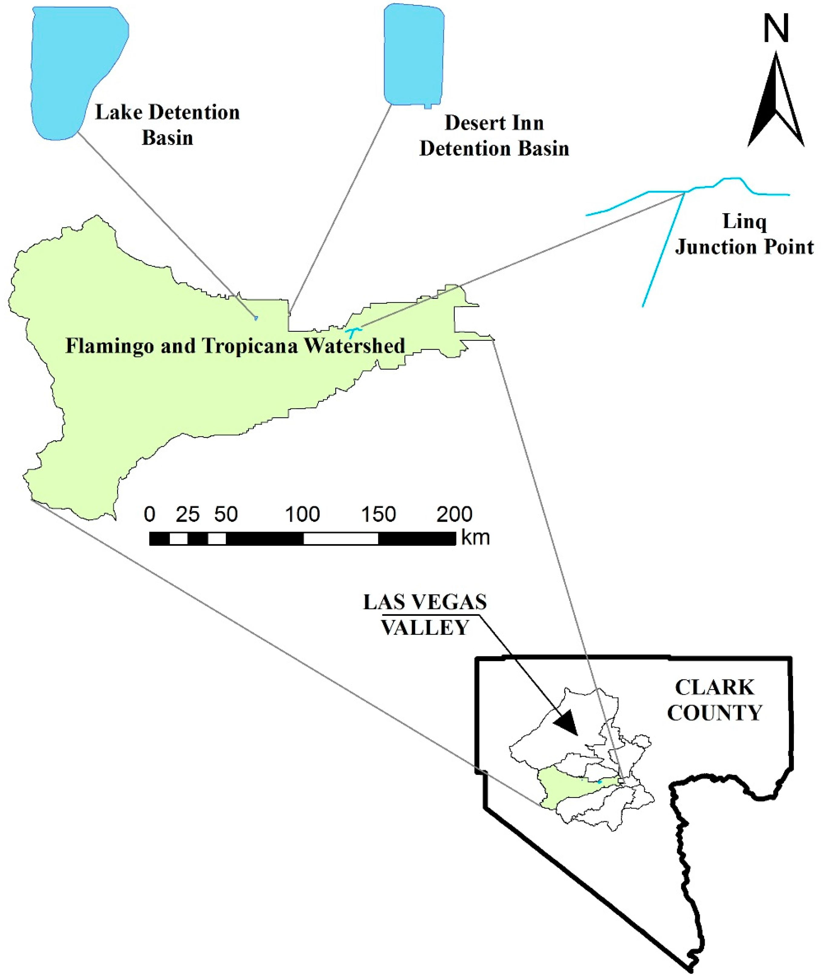
2. Study Area
3. Data and Model
- In the first phase, six RCM boundary conditions for a 25 year period (1979–2004) were used based on the data from the Atmospheric Model Intercomparison Project (AMIP-II) Reanalysis, conducted by the National Centers for Environmental Prediction and the U.S. Department of Energy (NCEP/DOE).
- In the second phase, four GCMs having time spans 30 years each for both historical climate data (1971–2000) and future climate data (2041–2070) were used for boundary conditions, taking into consideration the A2 scenarios from the Special Report on Emissions Scenarios (SRES) by the Intergovernmental Panel on Climate Change (IPCC) [44].
4. Methodology
5. Results
6. Discussion
7. Conclusions
Acknowledgments
Author Contributions
Conflicts of Interest
Abbreviations
| GCM | Global Climate Model |
| RCM | Regional Climate Model |
| CCRFCD | Clark County Regional Flood Control District |
| NARCCAP | North American Regional Climate Change Assessment Program |
| NARR | North American Regional Reanalysis |
| GEV | Generalized Extreme Value |
References
- Solomon, S.; Qin, D.; Manning, M.; Chen, Z.; Marquis, M.; Averyt, K.B.; Tignor, M.; Miller, H.L. Climate Change 2007-The Physical Science Basis: Contribution of Working Group I to the Fourth Assessment Report of the IPCC; Cambridge University Press: Cambridge, UK, 2007; Volume 4. [Google Scholar]
- Christensen, J.H.; Hewitson, B.; Busuioc, A.; Chen, A.; Gao, X.; Held, R.; Jones, R.; Kolli, R.K.; Kwon, W.; Laprise, R. Regional climate projections. In Climate Change, 2007: The Physical Science Basis. Contribution of Working Group I to the Fourth Assessment Report of the Intergovernmental Panel on Climate Change; Cambridge University Press: Cambridge, UK, 2007; Chapter 11; pp. 847–940. [Google Scholar]
- Sagarika, S.; Kalra, A.; Ahmad, S. Interconnections between oceanic–atmospheric indices and variability in the US streamflow. J. Hydrol. 2015, 525, 724–736. [Google Scholar] [CrossRef]
- Sagarika, S.; Kalra, A.; Ahmad, S. Pacific ocean SST and Z500 climate variability and western US seasonal streamflow. Int. J. Climatol. 2015, 36, 1515–1533. [Google Scholar] [CrossRef]
- Pathak, P.; Kalra, A.; Ahmad, S. Temperature and precipitation changes in the midwestern united states: Implications for water management. Int. J. Water Resour. Dev. 2016. [Google Scholar] [CrossRef]
- Tamaddun, K.; Kalra, A.; Ahmad, S. Identification of streamflow changes across the continental United States using variable record lengths. Hydrology 2016, 3, 24. [Google Scholar] [CrossRef]
- Olsson, J.; Berggren, K.; Olofsson, M.; Viklander, M. Applying climate model precipitation scenarios for urban hydrological assessment: A case study in Kalmar city, Sweden. Atmos. Res. 2009, 92, 364–375. [Google Scholar] [CrossRef]
- Easterling, D.R.; Evans, J.; Groisman, P.Y.; Karl, T.; Kunkel, K.E.; Ambenje, P. Observed variability and trends in extreme climate events: A brief review. Bull. Am. Meteorol. Soc. 2000, 81, 417–425. [Google Scholar] [CrossRef]
- Sagarika, S.; Kalra, A.; Ahmad, S. Evaluating the effect of persistence on long-term trends and analyzing step changes in streamflows of the continental United States. J. Hydrol. 2014, 517, 36–53. [Google Scholar] [CrossRef]
- Diodato, N.; Bellocchi, G.; Romano, N.; Chirico, G.B. How the aggressiveness of rainfalls in the Mediterranean lands is enhanced by climate change. Clim. Chang. 2011, 108, 591–599. [Google Scholar] [CrossRef]
- Konrad, C.P. Effects of Urban Development on Floods; US Department of the Interior: Washington, DC, USA, 2003; US Geological Survey Fact Sheet FS-076-03.
- Semadeni-Davies, A.; Hernebring, C.; Svensson, G.; Gustafsson, L.-G. The impacts of climate change and urbanization on drainage in Helsingborg, Sweden: Suburban stormwater. J. Hydrol. 2008, 350, 114–125. [Google Scholar] [CrossRef]
- Obeysekera, J.; Salas, J.D. Quantifying the uncertainty of design floods under nonstationary conditions. J. Hydrol. Eng. 2013, 19, 1438–1446. [Google Scholar] [CrossRef]
- Gilroy, K.L.; McCuen, R.H. A nonstationary flood frequency analysis method to adjust for future climate change and urbanization. J. Hydrol. 2012, 414, 40–48. [Google Scholar] [CrossRef]
- Rosenberg, E.A.; Keys, P.W.; Booth, D.B.; Hartley, D.; Burkey, J.; Steinemann, A.C.; Lettenmaier, D.P. Precipitation extremes and the impacts of climate change on stormwater infrastructure in Washington state. Clim. Chang. 2010, 102, 319–349. [Google Scholar] [CrossRef]
- Guo, Y. Updating rainfall idf relationships to maintain urban drainage design standards. J. Hydrol. Eng. 2006, 11, 506–509. [Google Scholar] [CrossRef]
- Carrier, C.A.; Kalra, A.; Ahmad, S. Long-range precipitation forecasts using paleoclimate reconstructions in the Western United States. J. Mt. Sci. 2016, 13, 614–632. [Google Scholar] [CrossRef]
- Pathak, P.; Kalra, A.; Ahmad, S.; Bernardez, M. Wavelet-aided analysis to estimate seasonal variability and dominant periodicities in temperature, precipitation, and streamflow in the Midwestern United States. Water Resour. Manag. 2016. [Google Scholar] [CrossRef]
- Tamaddun, K.A.; Kalra, A.; Ahmad, S. Wavelet analysis of Western US streamflow with ENSO and PDO. J. Water Clim. Chang. 2016. [Google Scholar] [CrossRef]
- Mailhot, A.; Duchesne, S. Design criteria of urban drainage infrastructures under climate change. J. Water Resour. Plan. Manag. 2010, 136, 201–208. [Google Scholar] [CrossRef]
- Milly, P.; Julio, B.; Malin, F.; Robert, M.; Zbigniew, W.; Dennis, P.; Ronald, J. Stationarity is dead. Ground Water News Views 2008, 4, 6–8. [Google Scholar]
- Wernstedt, K.; Carlet, F. Climate change, urban development, and storm water: Perspectives from the field. J. Water Resour. Plan. Manag. 2014, 140, 543–552. [Google Scholar] [CrossRef]
- Forsee, W.J.; Ahmad, S. Evaluating urban storm-water infrastructure design in response to projected climate change. J. Hydrol. Eng. 2011, 16, 865–873. [Google Scholar] [CrossRef]
- Hagemann, S.; Chen, C.; Clark, D.; Folwell, S.; Gosling, S.N.; Haddeland, I.; Hannasaki, N.; Heinke, J.; Ludwig, F.; Voss, F. Climate change impact on available water resources obtained using multiple global climate and hydrology models. Earth Syst. Dyn. 2013, 4, 129–144. [Google Scholar] [CrossRef]
- Fowler, H.; Blenkinsop, S.; Tebaldi, C. Linking climate change modelling to impacts studies: Recent advances in downscaling techniques for hydrological modelling. Int. J. Climatol. 2007, 27, 1547–1578. [Google Scholar] [CrossRef]
- Mearns, L.; Sain, S.; Leung, L.; Bukovsky, M.; McGinnis, S.; Biner, S.; Caya, D.; Arritt, R.; Gutowski, W.; Takle, E. Climate change projections of the North American regional climate change assessment program (NARCCAP). Clim. Chang. 2013, 120, 965–975. [Google Scholar] [CrossRef]
- Christensen, J.H.; Boberg, F.; Christensen, O.B.; Lucas-Picher, P. On the need for bias correction of regional climate change projections of temperature and precipitation. Geophys. Res. Lett. 2008. [Google Scholar] [CrossRef]
- Mearns, L.; Lettenmaier, D.; McGinnis, S. Uses of results of regional climate model experiments for impacts and adaptation studies: The example of NARCCAP. Curr. Clim. Chang. Rep. 2015, 1, 1–9. [Google Scholar] [CrossRef]
- Diaz-Nieto, J.; Wilby, R.L. A comparison of statistical downscaling and climate change factor methods: Impacts on low flows in the River Thames, United Kingdom. Clim. Chang. 2005, 69, 245–268. [Google Scholar] [CrossRef]
- Mailhot, A.; Duchesne, S.; Caya, D.; Talbot, G. Assessment of future change in intensity–duration–frequency (IDF) curves for Southern Quebec using the Canadian regional climate model (CRCM). J. Hydrol. 2007, 347, 197–210. [Google Scholar] [CrossRef]
- Zoppou, C. Review of urban storm water models. Environ. Model. Softw. 2001, 16, 195–231. [Google Scholar] [CrossRef]
- Gaber, N.; Foley, G.; Pascual, P.; Stiber, N.; Sunderland, E.; Cope, B.; Saleem, Z. Guidance on the Development, Evaluation, and Application of Environmental Models; US Environmental Protection Agency: Washington, DC, USA, March 2009.
- Elliott, A.; Trowsdale, S. A review of models for low impact urban stormwater drainage. Environ. Model. Softw. 2007, 22, 394–405. [Google Scholar] [CrossRef]
- Salvadore, E.; Bronders, J.; Batelaan, O. Hydrological modelling of urbanized catchments: A review and future directions. J. Hydrol. 2015, 529, 62–81. [Google Scholar] [CrossRef]
- Grum, M.; Jorgensen, A.; Johansen, R.; Linde, J. The effect of climate change on urban drainage: An evaluation based on regional climate model simulations. Water Sci. Technol. 2006, 54, 9–15. [Google Scholar] [CrossRef] [PubMed]
- He, J.; Valeo, C.; Bouchart, F. Enhancing urban infrastructure investment planning practices for a changing climate. Water Sci. Technol. 2006, 53, 13–20. [Google Scholar] [CrossRef] [PubMed]
- Brown, C. The end of reliability. J. Water Resour. Plan. Manag. 2010, 136, 143–145. [Google Scholar] [CrossRef]
- Jardine, A.; Merideth, R.; Black, M.; LeRoy, S. Assessment of Climate Change in the Southwest United States: A Report Prepared for the National Climate Assessment; Island Press: Washington, DC, USA, 2013. [Google Scholar]
- Levick, L.R.; Goodrich, D.C.; Hernandez, M.; Fonseca, J.; Semmens, D.J.; Stromberg, J.C.; Tluczek, M.; Leidy, R.A.; Scianni, M.; Guertin, D.P. The Ecological and Hydrological Significance of Ephemeral and Intermittent Streams in the Arid and Semi-Arid American Southwest; US Environmental Protection Agency: Washington, DC, USA, November 2008.
- Reilly, J.A.; Piechota, T.C. Actual storm events outperform synthetic design storms. A review of SCS curve number applicability. In Proceedings of the World Water and Environmental Resources Congress, Anchorage, AK, USA, 15–19 May 2005; American Society of Civil Engineers: Reston, VA, USA, 2005; pp. 1–13. Available online: http://www.egr.unlv.edu/~piechota/proceedings/reilly-piechota-ewri-2005.pdf (assessed on 5 October 2016). [Google Scholar]
- A Nevada Division of Water Resources Cooperative Technical Partner Project (NDWRCTPP), Nevada Flood Risk Portfolio: Flood Hazards and Flood Risk in Nevada’s Watersheds. 2013. Available online: http://water.nv.gov/programs/flood/hazards.pdf (assessed on 5 October 2016).
- Clark County Regional Flood Control District (CCRFCD). Regional Flood Control District Annual Report, Clark County, Nevada, 2014–2015; CCRFCD: Clark County, NV, USA, 2015; Available online: http://gustfront.ccrfcd.org/pdf_arch1/public%20information/annual%20reports/Annual%20Report%20-%2014-15.pdf (assessed on 5 October 2016).
- Mearns, L.; Gutowski, W.; Jones, R.; Leung, L.; McGinnis, S.; Nunes, A.; Qian, Y. The North American Regional Climate Change Assessment Program Dataset; National Center for Atmospheric Research Earth System Grid Data Portal: Boulder, CO, USA, 2007; Available online: https://www.earthsystemgrid.org/project/narccap.html (assessed on 5 October 2016).
- Mesinger, F.; DiMego, G.; Kalnay, E.; Mitchell, K.; Shafran, P.C.; Ebisuzaki, W.; Jovic, D.; Woollen, J.; Rogers, E.; Berbery, E.H. North American regional reanalysis. Bull. Am. Meteorol. Soc. 2006, 87, 343–360. [Google Scholar] [CrossRef]
- Mesinger, F.; DiMego, G.; Kalnay, E.; Shafran, P.; Ebisuzaki, W.; Jovic, D.; Woollen, J.; Mitchell, K.; Rogers, E.; Ek, M. NCEP North American Regional Reanalysis. In Proceedings of the 15th Symposium on Climate Change and Global Variations, 84th Conference of the AMS, Seattle, WA, USA, 11–15 January 2004.
- Kennedy, A.D.; Dong, X.; Xi, B.; Xie, S.; Zhang, Y.; Chen, J. A comparison of MERRA and NARR reanalyses with the DOE ARM SGP data. J. Clim. 2011, 24, 4541–4557. [Google Scholar] [CrossRef]
- Clark County Regional Flood Control District (CCRFCD). 2013 Las Vegas Valley Flood Control Master Plan Update; CCRFCD: Las Vegas, NV, USA, 2013. [Google Scholar]
- Clark County Regional Flood Control District (CCRFCD). Hydrologic Criteria and Drainage Design Manual; CCRFCD: Las Vegas, NV, USA, 1999. [Google Scholar]
- Miller, J.F.; Frederick, R.H.; Tracey, R.J. Precipitation-frequency Atlas of the Western United States; US Department of Commerce, National Oceanic & Atmospheric Administration: Washington, DC, USA, 1973.
- Clark County Regional Flood Control District (CCRFCD). 2008 Las Vegas Valley Flood Control Master Plan Update, Volume I and II; CCRFCD: Las Vegas, NV, USA, 2008. [Google Scholar]
- Hosking, J.R.M.; Wallis, J.R. Regional Frequency Analysis: An Approach Based on L-Moments; Cambridge University Press: Cambridge, UK, 1997; p. 224. [Google Scholar]
- Kendon, E.J.; Rowell, D.P.; Jones, R.G.; Buonomo, E. Robustness of future changes in local precipitation extremes. J. Clim. 2008, 21, 4280–4297. [Google Scholar] [CrossRef]
- Burn, D.H. Evaluation of regional flood frequency analysis with a region of influence approach. Water Resour. Res. 1990, 26, 2257–2265. [Google Scholar] [CrossRef]
- Castellarin, A.; Galeati, G.; Brandimarte, L.; Montanari, A.; Brath, A. Regional flow-duration curves: Reliability for ungauged basins. Adv. Water Resour. 2004, 27, 953–965. [Google Scholar] [CrossRef]
- Norbiato, D.; Borga, M.; Sangati, M.; Zanon, F. Regional frequency analysis of extreme precipitation in the eastern italian alps and the august 29, 2003 flash flood. J. Hydrol. 2007, 345, 149–166. [Google Scholar] [CrossRef]
- Fowler, H.; Wilby, R. Detecting changes in seasonal precipitation extremes using regional climate model projections: Implications for managing fluvial flood risk. Water Resour. Res. 2010, 46. [Google Scholar] [CrossRef]
- Institute of Hydrology. Flood Estimation Handbook; Institute of Hydrology: Wallingford, UK, 1999.
- Bonnin, G.M.; Martin, D.; Lin, B.; Parzybok, T.; Yekta, M.; Riley, D. Precipitation-17 Frequency Atlas of the United States, NOAA Atlas 14, NOAA; National Weather Service: Silver Spring, MD, USA, 2011; Volume 1.
- Kharin, V.V.; Zwiers, F.W. Changes in the extremes in an ensemble of transient climate simulations with a coupled atmosphere-ocean GCM. J. Clim. 2000, 13, 3760–3788. [Google Scholar] [CrossRef]
- Delgado, J.M.; Apel, H.; Merz, B. Flood trends and variability in the Mekong River. Hydrol. Earth Syst. Sci. 2010, 14, 407–418. [Google Scholar] [CrossRef]
- Gül, G.O.; Aşıkoğlu, Ö.L.; Gül, A.; Gülçem Yaşoğlu, F.; Benzeden, E. Nonstationarity in flood time series. J. Hydrol. Eng. 2013, 19, 1349–1360. [Google Scholar] [CrossRef]
- Katz, R.W.; Parlange, M.B.; Naveau, P. Statistics of extremes in hydrology. Adv. Water Resour. 2002, 25, 1287–1304. [Google Scholar] [CrossRef]
- Prosdocimi, I.; Kjeldsen, T.; Miller, J. Detection and attribution of urbanization effect on flood extremes using nonstationary flood-frequency models. Water Resour. Res. 2015, 51, 4244–4262. [Google Scholar] [CrossRef] [PubMed] [Green Version]
- Salas, J.D.; Obeysekera, J. Revisiting the concepts of return period and risk for nonstationary hydrologic extreme events. J. Hydrol. Eng. 2014, 19, 554–568. [Google Scholar] [CrossRef]
- Las Vegas Review-Journal. Las Vegas, NN, USA, 2016. Available online: http://www.reviewjournal.com/weather/4-rescued-during-record-breaking-rainfall-las-vegas-valley-photos (assessed on 5 October 2016).
- PressReader Online Journal. British Columbia, Canada, 2016. Available online: http://www.pressreader.com/usa/las-vegas-review-journal-sunday/20160410/282067686091968 (assessed on 5 October 2016).
- Wehner, M.F. Very extreme seasonal precipitation in the narccap ensemble: Model performance and projections. Clim. Dyn. 2013, 40, 59–80. [Google Scholar] [CrossRef]
- Acharya, A.; Lamb, K.; Piechota, T.C. Impacts of climate change on extreme precipitation events over Flamingo Tropicana Watershed. J. Am. Water Resour. Assoc. 2013, 49, 359–370. [Google Scholar] [CrossRef]


| Model Combination (GCM/RCM) | GCM | RCM |
|---|---|---|
| CGCM3/CRCM | Third Generation Coupled Global Climate Model | Canadian Regional Climate Model |
| CGCM3/RCM3 | Third Generation Coupled Global Climate Model | Regional Climate Model version 3 |
| CGCM3/WRFG | Third Generation Coupled Global Climate Model | Weather Research and Forecasting Model |
| CCSM/CRCM | Community Climate System Model | Canadian Regional Climate Model |
| CCSM/WRFG | Community Climate System Model | Weather Research and Forecasting Model |
| CCSM/MM5I | Community Climate System Model | MM5, the PSU/NCAR Mesoscale Model |
| HaDCM3/HRM3 | Hadley Centre Coupled Global Climate Model | Hadley Regional model 3 |
| HaDCM3/MM5I | Hadley Centre Coupled Global Climate Model | MM5–PSU/NCAR Mesoscale Model |
| GFDL/HRM3 | Geophysical Fluid Dynamics Laboratory | Hadley Regional model 3 |
| GFDL/RCM3 | Geophysical Fluid Dynamics Laboratory | Regional Climate Model version 3 |
| GFDL/ECPC | Geophysical Fluid Dynamics Laboratory | Experimental Climate Prediction Center |
| Time slice GFDL | Geophysical Fluid Dynamics Laboratory | |
| Time slice CCSM | Community Climate System Model |
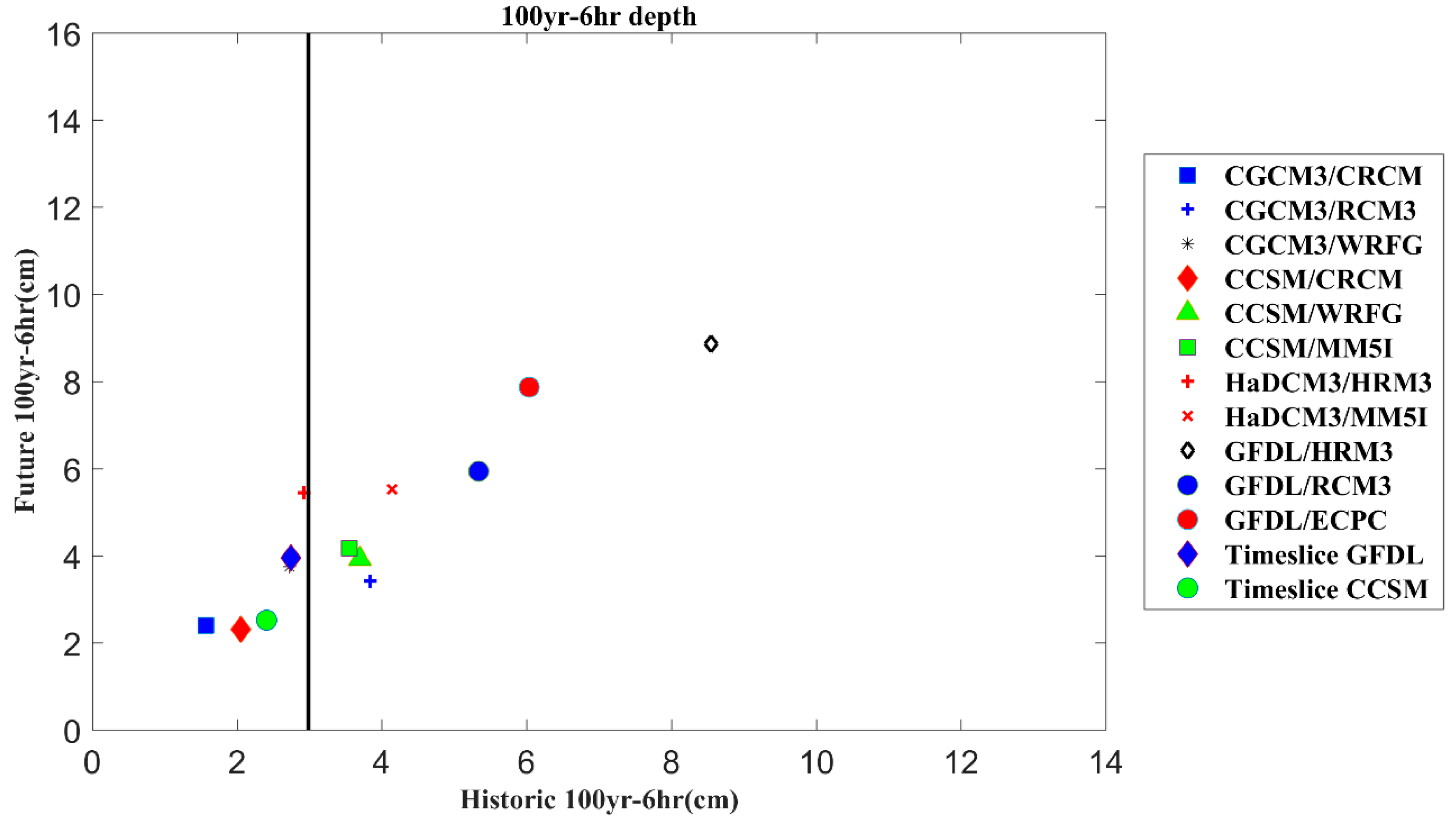
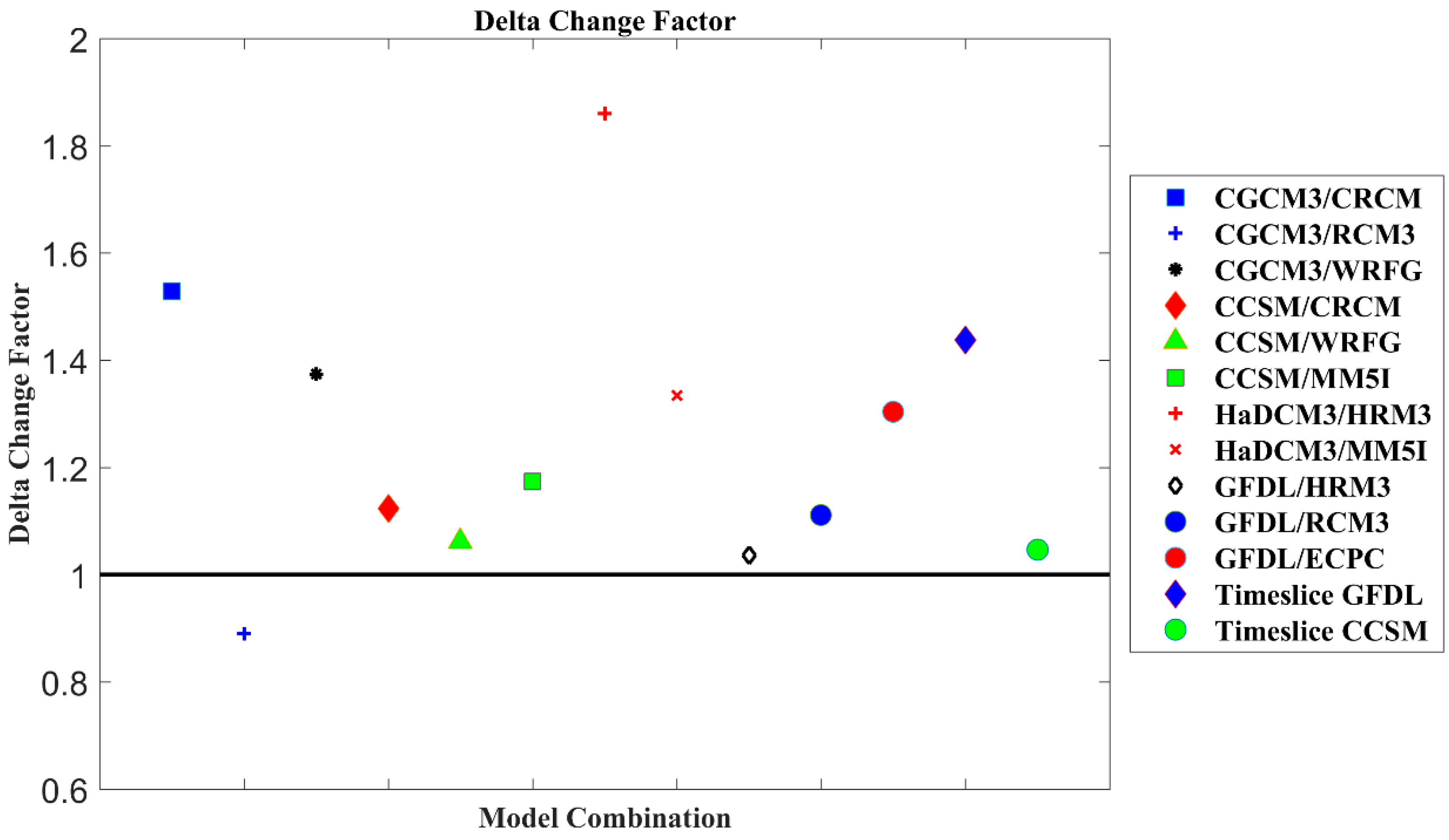
| Model Combination GCM/RCM | Historic 100yr-6hr Depth (cm) | Future 100yr-6hr Depth (cm) | Delta Change Factor |
|---|---|---|---|
| NARR | 2.98 | - | - |
| CGCM3/CRCM | 1.57 | 2.40 | 1.53 |
| CGCM3/RCM3 | 3.84 | 3.42 | 0.89 |
| CGCM3/WRFG | 2.72 | 3.74 | 1.37 |
| CCSM/CRCM | 2.05 | 2.30 | 1.12 |
| CCSM/WRFG | 3.70 | 3.92 | 1.06 |
| CCSM/MM5I | 3.55 | 4.17 | 1.17 |
| HaDCM3/HRM3 | 2.93 | 5.45 | 1.86 |
| HaDCM3/MM5I | 4.14 | 5.52 | 1.33 |
| GFDL/HRM3 | 8.55 | 8.86 | 1.04 |
| GFDL/RCM3 | 5.34 | 5.93 | 1.11 |
| GFDL/ECPC | 6.03 | 7.87 | 1.30 |
| Time slice GFDL | 2.74 | 3.94 | 1.44 |
| Time slice CCSM | 2.41 | 2.52 | 1.05 |
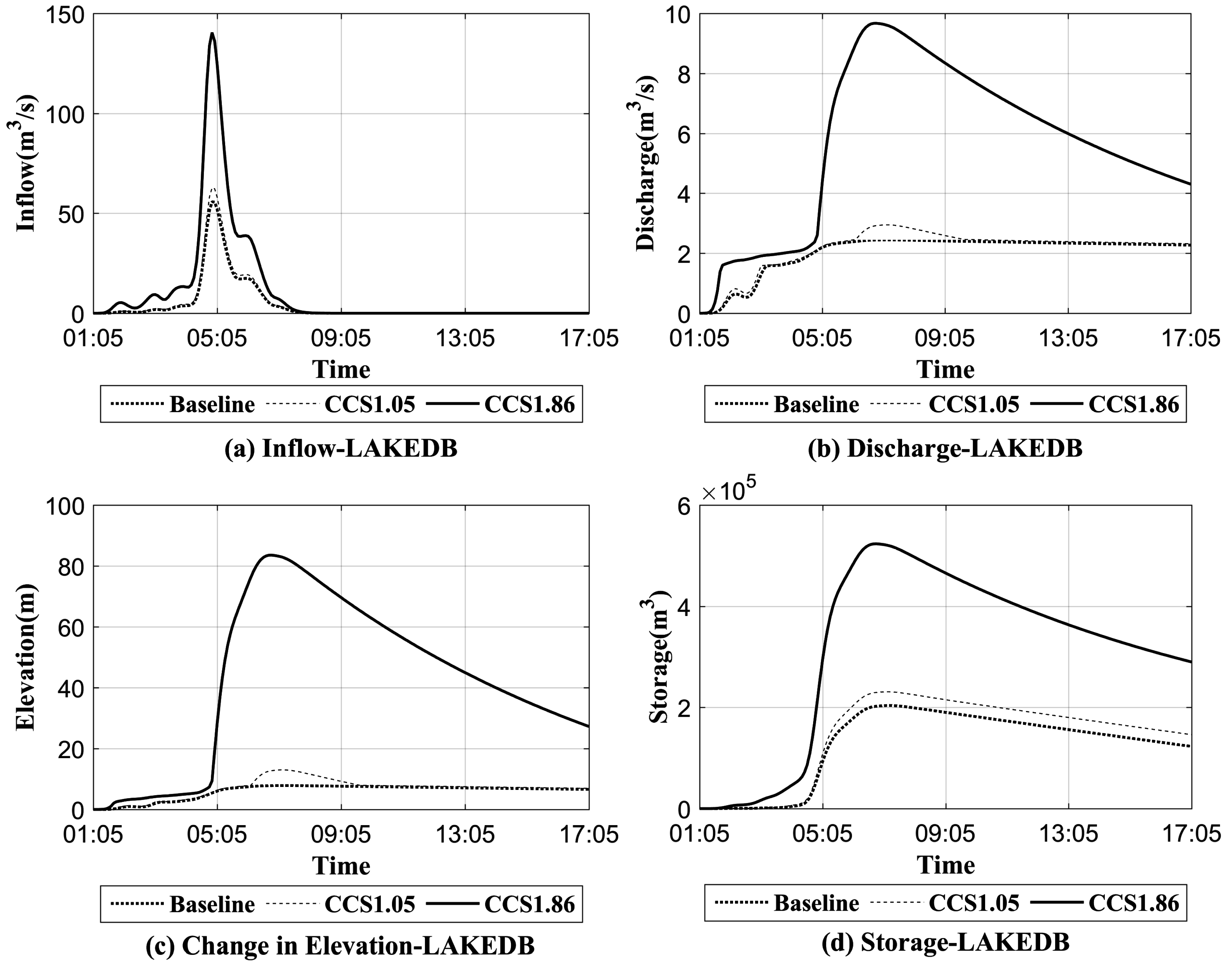
| Element | Scenario | Inflow (m3/s) | Storage (m3) | Change in Elevation (m) | Outflow (m3/s) |
|---|---|---|---|---|---|
| LAKEDB | Design | 55.95 | 203,524.20 | 7.83 | 2.72 |
| Baseline | 55.73 | 203,770.90 | 7.83 | 2.45 | |
| CCS 1.05 | 60.26 | 221,162.96 | 10.67 | 2.73 | |
| CCS 1.86 | 135.71 | 504,863.36 | 79.10 | 9.25 | |
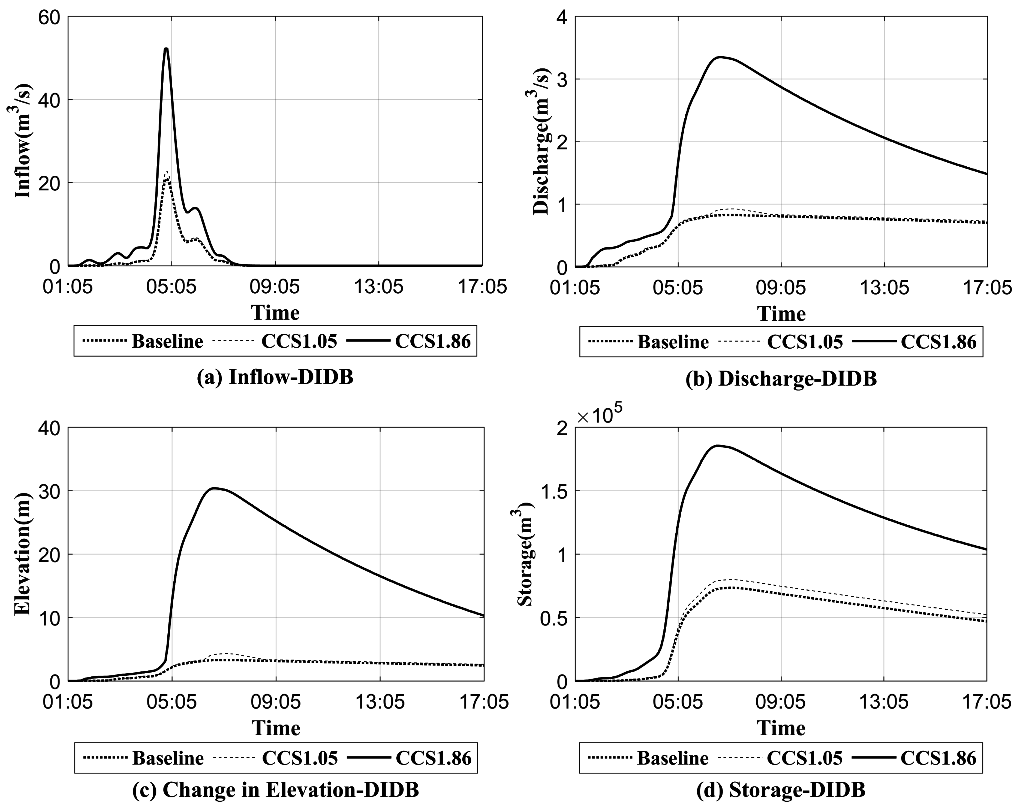
| DIDB | Design | 21.07 | 76,475.76 | 3.26 | 0.82 |
| Baseline | 20.93 | 73,392.06 | 3.26 | 0.82 | |
| CCS 1.05 | 22.66 | 79,806.16 | 4.30 | 0.92 | |
| CCS 1.86 | 52.20 | 185,268.70 | 30.36 | 3.35 | |
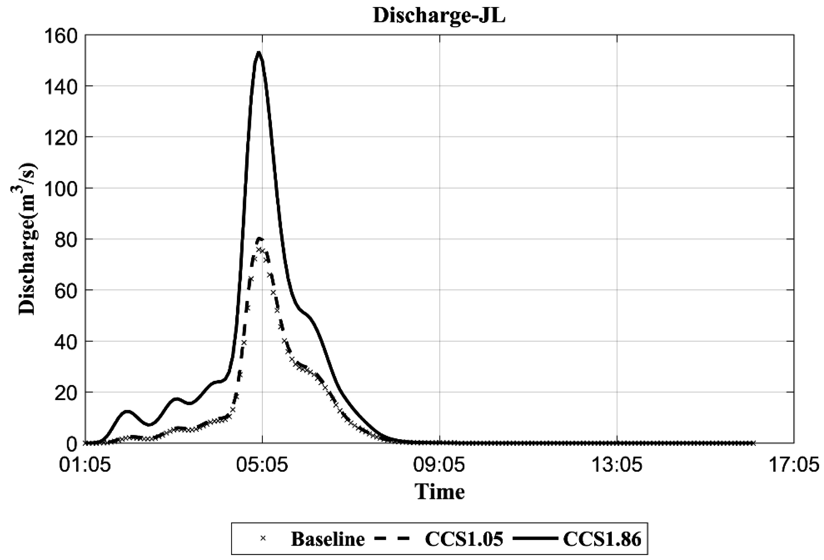
| DIDB | Design | 76.17 | - | - | - |
| Baseline | 75.71 | - | - | - | |
| CCS 1.05 | 80.25 | - | - | - | |
| CCS 1.86 | 153.32 | - | - | - |
© 2016 by the authors; licensee MDPI, Basel, Switzerland. This article is an open access article distributed under the terms and conditions of the Creative Commons Attribution (CC-BY) license (http://creativecommons.org/licenses/by/4.0/).
Share and Cite
Thakali, R.; Kalra, A.; Ahmad, S. Understanding the Effects of Climate Change on Urban Stormwater Infrastructures in the Las Vegas Valley. Hydrology 2016, 3, 34. https://doi.org/10.3390/hydrology3040034
Thakali R, Kalra A, Ahmad S. Understanding the Effects of Climate Change on Urban Stormwater Infrastructures in the Las Vegas Valley. Hydrology. 2016; 3(4):34. https://doi.org/10.3390/hydrology3040034
Chicago/Turabian StyleThakali, Ranjeet, Ajay Kalra, and Sajjad Ahmad. 2016. "Understanding the Effects of Climate Change on Urban Stormwater Infrastructures in the Las Vegas Valley" Hydrology 3, no. 4: 34. https://doi.org/10.3390/hydrology3040034